See pages 1 of Main.pdf See pages 2 of Main.pdf See pages 3 of Main.pdf See pages 4 of Main.pdf See pages 5 of Main.pdf See pages 6 of Main.pdf See pages 7 of Main.pdf See pages 8 of Main.pdf See pages 9 of Main.pdf See pages 10 of Main.pdf See pages 11 of Main.pdf See pages 12 of Main.pdf See pages 13 of Main.pdf See pages 14 of Main.pdf See pages 15 of Main.pdf

Supplementary information for: Selective scattering between Floquet-Bloch and Volkov states in a topological insulator

Fahad Mahmood, Ching-Kit Chan, Zhanybek Alpichshev, Dillon Gardner, Young Lee, Patrick A. Lee, Nuh Gedik

I Theoretical details

In this section, we provide details of calculations for the Tr-ARPES intensity from driven surface states of a topological insulator. We consider the intrinsic Floquet states attributed by the drive, the spin-probe effect on the photoemission matrix elements, and the influence of LAPE. These combined contributions lead to the theoretical results presented in the main text.

The effective Hamiltonian describing the undriven surface states of a 3D topological insulator is given by:

$\displaystyle H$ $\displaystyle=$ βˆ‘k=kx,ky(ck,↑†ck,↓†)​(0ℏ​vf​(βˆ’i​kxβˆ’ky)ℏ​vf​(i​kxβˆ’ky)0)​(ck,↑ck,↓),subscriptπ‘˜subscriptπ‘˜π‘₯subscriptπ‘˜π‘¦matrixsuperscriptsubscriptπ‘π‘˜β†‘β€ superscriptsubscriptπ‘π‘˜β†“β€ matrix0Planck-constant-over-2-pisubscript𝑣𝑓𝑖subscriptπ‘˜π‘₯subscriptπ‘˜π‘¦Planck-constant-over-2-pisubscript𝑣𝑓𝑖subscriptπ‘˜π‘₯subscriptπ‘˜π‘¦0matrixsubscriptπ‘π‘˜β†‘subscriptπ‘π‘˜β†“\displaystyle\sum_{k=k_{x},k_{y}}\begin{pmatrix}c_{k,\uparrow}^{\dagger}&c_{k,\downarrow}^{\dagger}\end{pmatrix}\begin{pmatrix}0&\hbar v_{f}(-ik_{x}-k_{y})\\ \hbar v_{f}(ik_{x}-k_{y})&0\end{pmatrix}\begin{pmatrix}c_{k,\uparrow}\\ c_{k,\downarrow}\end{pmatrix}, (1)

where ck,σ†superscriptsubscriptπ‘π‘˜πœŽβ€ c_{k,\sigma}^{\dagger} creates a bare electron with momentum $k$ and pseudospin $\sigma$. Diagonalizing the Hamiltonian would give the canonical linear dispersion of surface states, i.e. $\epsilon_{\pm}(\vec{k})=\pm\hbar v_{f}|\vec{k}|$. The laser drive is introduced through the Peierls’ substitution: $v_{f}\vec{k}\rightarrow\vec{K}(t)=v_{f}(\vec{k}+e\vec{A}(t))$, with $\vec{A}(t)=A_{0}g(t)\left(a_{x}\cos(\omega t),a_{y}\sin(\omega t)\right)$. $A_{0}$ is the peak pump field strength, $g(t)$ describes the Gaussian pump envelope and $0\leq a_{x/y}\leq 1$ characterize its polarizations. We use $\beta=ev_{f}A_{0}/\omega$ as the dimensionless Floquet parameter in the main text.

The general idea of Floquet-Volkov transition has been studied by Park park14 . Using a scattering approach, it was estimated that the $n$-th Floquet sideband has an intensity (in our notation):

$\displaystyle I(\vec{k},E)\approx J_{n}\left\{\left|\lambda\beta\left(\cos\theta_{a}\cos\theta+i\sin\theta_{a}\sin\theta\right)-\alpha\right|\right\}^{2}$ (2)

as a function of the momentum angle $\theta=\tan^{-1}(k_{y}/k_{x})$ and the polarization angle $\theta_{a}=\tan^{-1}(a_{y}/a_{x})$. $\lambda=\pm$ denotes the upper and lower bands, and $\alpha$ is a LAPE parameter to be defined later. However, we find that this formula does not fit well with the data because of approximations made (specifically, the components of $\vec{A}(t)$ perpendicular to $\vec{k}$ are neglected park14 ), and more importantly, the missing of the spin-probe effect. Therefore, we introduce here an alternative method, based on the non-equilibrium Green’s function freericks09 , that naturally incorporates the Floquet, the LAPE and the spin-probe effects and accurately describes our photoemission experiments.

I.1 Tr-ARPES dynamics

The pump-probe Tr-ARPES measures the photoelectron correlations freericks09 :

I​(kβ†’,E)=∫titf𝑑tβ€‹βˆ«0tfβˆ’t𝑑τ​s​(t)​s​(t+Ο„)β€‹βˆ‘Οƒ1,Οƒ2,ΟƒfMkβˆ—β€‹(Οƒf,Οƒ1)​Mk​(Οƒf,Οƒ2)​2​Re​[⟨ck,Οƒ1†​(t+Ο„)​ck,Οƒ2​(t)βŸ©β€‹eβˆ’i​E​τ/ℏ],πΌβ†’π‘˜πΈsuperscriptsubscriptsubscript𝑑𝑖subscript𝑑𝑓differential-d𝑑superscriptsubscript0subscript𝑑𝑓𝑑differential-dπœπ‘ π‘‘π‘ π‘‘πœsubscriptsubscript𝜎1subscript𝜎2subscriptπœŽπ‘“superscriptsubscriptπ‘€π‘˜subscriptπœŽπ‘“subscript𝜎1subscriptπ‘€π‘˜subscriptπœŽπ‘“subscript𝜎22Redelimited-[]delimited-⟨⟩superscriptsubscriptπ‘π‘˜subscript𝜎1β€ π‘‘πœsubscriptπ‘π‘˜subscript𝜎2𝑑superscriptπ‘’π‘–πΈπœPlanck-constant-over-2-pi\displaystyle I(\vec{k},E)=\int_{t_{i}}^{t_{f}}dt\int_{0}^{t_{f}-t}d\tau s(t)s(t+\tau)\sum_{\sigma_{1},\sigma_{2},\sigma_{f}}M_{k}^{*}(\sigma_{f},\sigma_{1})M_{k}(\sigma_{f},\sigma_{2})2~{}\text{Re}\left[\langle c_{k,\sigma_{1}}^{\dagger}(t+\tau)c_{k,\sigma_{2}}(t)\rangle e^{-iE\tau/\hbar}\right], (3)

caused by a probe field with a normalized Gaussian envelope $s(t)$, an initial time $t_{i}$ and a final time $t_{f}$. The expectation value is taken with respect to the wavefunction of the driven system. This expression describes a virtual process where an electron is photoexcited at time $t$ and then returns at time $t+\tau$. The matrix elements $M_{k}(\sigma^{\prime},\sigma)$ correspond to transitions from spin $\sigma$ to $\sigma^{\prime}$ and depend on the details of system-probe interactions. In the absence of spin-probe coupling, we have $M_{k}(\sigma^{\prime},\sigma)\propto\delta_{\sigma,\sigma^{\prime}}$ and the Tr-ARPES intensity becomes:

I0​(kβ†’,E)∝∫titf𝑑tβ€‹βˆ«0tfβˆ’t𝑑τ​s​(t)​s​(t+Ο„)β€‹βˆ‘Οƒ2​Re​[⟨ck,σ†​(t+Ο„)​ck,σ​(t)βŸ©β€‹eβˆ’i​E​τ/ℏ].proportional-tosubscript𝐼0β†’π‘˜πΈsuperscriptsubscriptsubscript𝑑𝑖subscript𝑑𝑓differential-d𝑑superscriptsubscript0subscript𝑑𝑓𝑑differential-dπœπ‘ π‘‘π‘ π‘‘πœsubscript𝜎2Redelimited-[]delimited-⟨⟩superscriptsubscriptπ‘π‘˜πœŽβ€ π‘‘πœsubscriptπ‘π‘˜πœŽπ‘‘superscriptπ‘’π‘–πΈπœPlanck-constant-over-2-pi\displaystyle I_{0}(\vec{k},E)\propto\int_{t_{i}}^{t_{f}}dt\int_{0}^{t_{f}-t}d\tau s(t)s(t+\tau)\sum_{\sigma}2~{}\text{Re}\left[\langle c_{k,\sigma}^{\dagger}(t+\tau)c_{k,\sigma}(t)\rangle e^{-iE\tau/\hbar}\right]. (4)

In the equilibrium limit, and for a uniform probe, this expression reduces to: I0​(kβ†’,E)∼(tfβˆ’ti)β€‹βˆ«0βˆžπ‘‘Ο„β€‹βˆ‘Οƒ2​Re​[⟨ck,σ†​(Ο„)​ck,σ​(0)βŸ©β€‹eβˆ’i​E​τ/ℏ]similar-tosubscript𝐼0β†’π‘˜πΈsubscript𝑑𝑓subscript𝑑𝑖superscriptsubscript0differential-d𝜏subscript𝜎2Redelimited-[]delimited-⟨⟩superscriptsubscriptπ‘π‘˜πœŽβ€ πœsubscriptπ‘π‘˜πœŽ0superscriptπ‘’π‘–πΈπœPlanck-constant-over-2-piI_{0}(\vec{k},E)\sim(t_{f}-t_{i})\int_{0}^{\infty}d\tau\sum_{\sigma}2~{}\text{Re}[\langle c_{k,\sigma}^{\dagger}(\tau)c_{k,\sigma}(0)\rangle e^{-iE\tau/\hbar}], which is proportional to the standard lesser Green’s function freericks09 .

To calculate Eq.Β (4), we need the equation of motions for the two-time correlation functions. They are:

ddβ€‹Ο„β€‹βŸ¨ck,↑†​(t+Ο„)​ck,↑⁣/↓​(t)βŸ©π‘‘π‘‘πœdelimited-⟨⟩superscriptsubscriptπ‘π‘˜β†‘β€ π‘‘πœsubscriptπ‘π‘˜β†‘absent↓𝑑\displaystyle\frac{d}{d\tau}\langle c_{k,\uparrow}^{\dagger}(t+\tau)c_{k,\uparrow/\downarrow}(t)\rangle $\displaystyle=$ (βˆ’Kx​(t+Ο„)βˆ’i​Ky​(t+Ο„))β€‹βŸ¨ck,↓†​(t+Ο„)​ck,↑⁣/↓​(t)⟩,subscript𝐾π‘₯π‘‘πœπ‘–subscriptπΎπ‘¦π‘‘πœdelimited-⟨⟩superscriptsubscriptπ‘π‘˜β†“β€ π‘‘πœsubscriptπ‘π‘˜β†‘absent↓𝑑\displaystyle(-K_{x}(t+\tau)-iK_{y}(t+\tau))\langle c_{k,\downarrow}^{\dagger}(t+\tau)c_{k,\uparrow/\downarrow}(t)\rangle,
ddβ€‹Ο„β€‹βŸ¨ck,↓†​(t+Ο„)​ck,↑⁣/↓​(t)βŸ©π‘‘π‘‘πœdelimited-⟨⟩superscriptsubscriptπ‘π‘˜β†“β€ π‘‘πœsubscriptπ‘π‘˜β†‘absent↓𝑑\displaystyle\frac{d}{d\tau}\langle c_{k,\downarrow}^{\dagger}(t+\tau)c_{k,\uparrow/\downarrow}(t)\rangle $\displaystyle=$ (Kx​(t+Ο„)βˆ’i​Ky​(t+Ο„))β€‹βŸ¨ck,↑†​(t+Ο„)​ck,↑⁣/↓​(t)⟩.subscript𝐾π‘₯π‘‘πœπ‘–subscriptπΎπ‘¦π‘‘πœdelimited-⟨⟩superscriptsubscriptπ‘π‘˜β†‘β€ π‘‘πœsubscriptπ‘π‘˜β†‘absent↓𝑑\displaystyle(K_{x}(t+\tau)-iK_{y}(t+\tau))\langle c_{k,\uparrow}^{\dagger}(t+\tau)c_{k,\uparrow/\downarrow}(t)\rangle. (5)

The initial condition at $\tau=0$ is determined by the equal-time correlations ⟨ck,σ†​(t)​ck,σ′​(t)⟩delimited-⟨⟩superscriptsubscriptπ‘π‘˜πœŽβ€ π‘‘subscriptπ‘π‘˜superscriptπœŽβ€²π‘‘\langle c_{k,\sigma}^{\dagger}(t)c_{k,\sigma^{\prime}}(t)\rangle. Generally speaking, the initial condition ⟨ck,σ†​(t)​ck,σ′​(t)⟩delimited-⟨⟩superscriptsubscriptπ‘π‘˜πœŽβ€ π‘‘subscriptπ‘π‘˜superscriptπœŽβ€²π‘‘\langle c_{k,\sigma}^{\dagger}(t)c_{k,\sigma^{\prime}}(t)\rangle depends on $t$ due to the non-equilibrium nature of the problem. However, in the main text, we are mostly interested in the cases of $|\vec{k}|\leq k_{F}$, where both the lower and upper band of the undriven Dirac cone are filled so that no vertical transition is allowed by the drive. In this regime, we have ⟨ck,σ†​(t)​ck,σ′​(t)⟩=⟨ck,σ†​(0)​ck,σ′​(0)⟩=δσ,Οƒβ€²delimited-⟨⟩superscriptsubscriptπ‘π‘˜πœŽβ€ π‘‘subscriptπ‘π‘˜superscriptπœŽβ€²π‘‘delimited-⟨⟩superscriptsubscriptπ‘π‘˜πœŽβ€ 0subscriptπ‘π‘˜superscriptπœŽβ€²0subscriptπ›ΏπœŽsuperscriptπœŽβ€²\langle c_{k,\sigma}^{\dagger}(t)c_{k,\sigma^{\prime}}(t)\rangle=\langle c_{k,\sigma}^{\dagger}(0)c_{k,\sigma^{\prime}}(0)\rangle=\delta_{\sigma,\sigma^{\prime}}. On the other hand, for $|\vec{k}|>k_{F}$, ⟨ck,σ†​(t)​ck,σ′​(t)⟩delimited-⟨⟩superscriptsubscriptπ‘π‘˜πœŽβ€ π‘‘subscriptπ‘π‘˜superscriptπœŽβ€²π‘‘\langle c_{k,\sigma}^{\dagger}(t)c_{k,\sigma^{\prime}}(t)\rangle becomes t-dependent and can be computed by solving its equation of motion using the driven Hamiltonian.

Since the relaxation time scale is much longer than that of the drive in our experiment, dissipative effects are negligible. However, when dissipation becomes important, we have to augment Eq.Β (5) with relaxation terms based on the master equation formalism dehghani14 or the kinetic approach seetharam15 .

I.2 Spin-probe effect

When the probe couples to the spin, one has to compute the matrix elements $M_{k}(f,i)=\langle f|\vec{P}_{k}\cdot\vec{A}_{\text{probe}}(t)|i\rangle$ wang11 . In accordance with our experimental setup, we consider a p-polarized probe such that $\vec{A}_{\text{probe}}=(A_{x},0,A_{z})$. In general, $\vec{P}_{k}$ is some generalized momentum and depends on the system details and spin-orbit couplings. However, by considering the mirror reflection symmetry and the three-fold rotational symmetry wang11 , one can simplify the matrix elements to (in the basis of spin up and down):

$\displaystyle M_{k}=i\begin{pmatrix}b_{k}A_{z}&\frac{a_{k}A_{x}}{2}\\ -\frac{a_{k}A_{x}}{2}&b_{k}A_{z}\end{pmatrix},$ (6)

where $a_{k}$ and $b_{k}$ are real coefficients. Using these matrix elements, Eq.Β (3) becomes:

I​(kβ†’,E)∝I0​(kβ†’,E)+cS​Pβ€‹βˆ«titf𝑑tβ€‹βˆ«0tfβˆ’t𝑑τ​s​(t)​s​(t+Ο„)​2​Re​[eβˆ’i​E​τ/β„β€‹βŸ¨βˆ’i​ck,↑†​(t+Ο„)​ck,↓​(t)+i​ck,↓†​(t+Ο„)​ck,↑​(t)⟩],proportional-toπΌβ†’π‘˜πΈsubscript𝐼0β†’π‘˜πΈsubscript𝑐𝑆𝑃superscriptsubscriptsubscript𝑑𝑖subscript𝑑𝑓differential-d𝑑superscriptsubscript0subscript𝑑𝑓𝑑differential-dπœπ‘ π‘‘π‘ π‘‘πœ2Redelimited-[]superscriptπ‘’π‘–πΈπœPlanck-constant-over-2-pidelimited-βŸ¨βŸ©π‘–superscriptsubscriptπ‘π‘˜β†‘β€ π‘‘πœsubscriptπ‘π‘˜β†“π‘‘π‘–superscriptsubscriptπ‘π‘˜β†“β€ π‘‘πœsubscriptπ‘π‘˜β†‘π‘‘\displaystyle I(\vec{k},E)\propto I_{0}(\vec{k},E)+c_{SP}\int_{t_{i}}^{t_{f}}dt\int_{0}^{t_{f}-t}d\tau s(t)s(t+\tau)2~{}\text{Re}\left[e^{-iE\tau/\hbar}\langle-ic_{k,\uparrow}^{\dagger}(t+\tau)c_{k,\downarrow}(t)+ic_{k,\downarrow}^{\dagger}(t+\tau)c_{k,\uparrow}(t)\rangle\right], (7)

where the parameter $c_{SP}=[ia_{k}b_{k}A_{z}^{*}A_{x}+\text{c.c.}]/[a_{k}^{2}|A_{x}|^{2}/2+2b_{k}^{2}|A_{z}|^{2}]$ characterizes the spin-probe effect. Note that the spin-probe effect only couples to the $S_{y}$ component in this setting of a p-polarized probe. Because of the spin-momentum locking, we have $S_{y}\sim\cos\theta$ and thus the spin-probe effect is most prominent at $\theta=0,\pi$, i.e. along the $k_{x}$ direction. For a probe with a general polarization, the $S_{x}$ and $S_{z}$ components can also be involved ($S_{x}$ couples to $A_{y,z}$ and $S_{z}$ couples to $A_{x,y}$).

We can extract the single coefficient $c_{SP}$ from the pre-time zero data. In the equilibrium limit, for a p-polarized probe, we recover the static result: $I-I_{0}\propto c_{SP}S_{y}$ wang11 .

I.3 LAPE

The Laser-Assisted Photoemission Effect (LAPE) is caused by the interference between the pump and the photoexcited electrons. The corresponding Hamiltonian is $H_{\text{LAPE}}=\hbar e\vec{v}_{0}\cdot\vec{A}_{\text{pump}}(t)$, where $\vec{v}_{0}$ is the free photoelectron velocity. Consequentially, the two-time correlation function in the Tr-ARPES intensity [Eq.Β (3)] picks up an additional phase:

$\displaystyle e^{i\Theta(\alpha_{k},t,\tau)}$ $\displaystyle=$ $\displaystyle e^{-i\int_{t}^{t+\tau}dt^{\prime}H_{\text{LAPE}}(t^{\prime})/\hbar}$ (8)
$\displaystyle=$ $\displaystyle\exp\{-i(\alpha_{k_{x}}+\alpha_{k_{z}})[\sin\omega(t+\tau)-\sin\omega t]+i\alpha_{k_{y}}[\cos\omega(t+\tau)-\cos\omega t]\},$

where $\alpha_{k_{i}}=ev_{0,i}A_{\text{pump},i}/\omega$. Note that the pump field can have a $z$-component contribution to the LAPE. In fact, for the p-polarized pump experiment, we have $\alpha_{k_{z}}\gg\alpha_{k_{x}/k_{y}}$, since the pump field has a larger $z$-component and $|v_{0,z}|\sim v_{f}\gg|v_{0,x/y}|$. Thus, we set $\alpha_{k_{z}}=\alpha$ and $\alpha_{k_{x}/k_{y}}=0$ in the main text. On the other hand, in the s-polarized pump case, all $\alpha_{k}$ are negligible.

Therefore, for a p-polarized probe, the Tr-ARPES intensity, including the spin-probe ($c_{SP}$) and the LAPE ($\alpha_{k}$) effects, is given by:

I​(kβ†’,E)∝∫titf𝑑tβ€‹βˆ«0tfβˆ’t𝑑τ​s​(t)​s​(t+Ο„)​2​Re​{eβˆ’i​E​τ/ℏ​eiβ€‹Ξ˜β€‹(Ξ±k,t,Ο„)​[S0​(t,Ο„)+cS​P​Sy​(t,Ο„)]},proportional-toπΌβ†’π‘˜πΈsuperscriptsubscriptsubscript𝑑𝑖subscript𝑑𝑓differential-d𝑑superscriptsubscript0subscript𝑑𝑓𝑑differential-dπœπ‘ π‘‘π‘ π‘‘πœ2Resuperscriptπ‘’π‘–πΈπœPlanck-constant-over-2-pisuperscriptπ‘’π‘–Ξ˜subscriptπ›Όπ‘˜π‘‘πœdelimited-[]subscript𝑆0π‘‘πœsubscript𝑐𝑆𝑃subscriptπ‘†π‘¦π‘‘πœ\displaystyle I(\vec{k},E)\propto\int_{t_{i}}^{t_{f}}dt\int_{0}^{t_{f}-t}d\tau s(t)s(t+\tau)2~{}\text{Re}\left\{e^{-iE\tau/\hbar}e^{i\Theta(\alpha_{k},t,\tau)}\left[S_{0}(t,\tau)+c_{SP}S_{y}(t,\tau)\right]\right\}, (9)

where S0​(t,Ο„)=βˆ‘ΟƒβŸ¨ck,σ†​(t+Ο„)​ck,σ​(t)⟩subscript𝑆0π‘‘πœsubscript𝜎delimited-⟨⟩superscriptsubscriptπ‘π‘˜πœŽβ€ π‘‘πœsubscriptπ‘π‘˜πœŽπ‘‘S_{0}(t,\tau)=\sum_{\sigma}\langle c_{k,\sigma}^{\dagger}(t+\tau)c_{k,\sigma}(t)\rangle and Sy​(t,Ο„)=βŸ¨βˆ’i​ck,↑†​(t+Ο„)​ck,↓​(t)+i​ck,↓†​(t+Ο„)​ck,↑​(t)⟩subscriptπ‘†π‘¦π‘‘πœdelimited-βŸ¨βŸ©π‘–superscriptsubscriptπ‘π‘˜β†‘β€ π‘‘πœsubscriptπ‘π‘˜β†“π‘‘π‘–superscriptsubscriptπ‘π‘˜β†“β€ π‘‘πœsubscriptπ‘π‘˜β†‘π‘‘S_{y}(t,\tau)=\langle-ic_{k,\uparrow}^{\dagger}(t+\tau)c_{k,\downarrow}(t)+ic_{k,\downarrow}^{\dagger}(t+\tau)c_{k,\uparrow}(t)\rangle can be obtained by solving Eq.Β (5). The theoretical curves in Figure 3e and 4d in the main text are calculated from this expression.

I.4 Exactly solvable case: parity of Floquet-LAPE states

Analytical solutions are available for special cases where $\vec{k}\parallel\vec{A}(t)$. Here we particularly study the situation of (1) $\pm k_{x}$ for a p-polarized pump, and (2) $\pm k_{y}$ for a s-polarized pump, in order to understand the parity of the Tr-ARPES signals with and without the LAPE effect. We use uniform pump and probe to simplify the notations.

I.4.1 Without LAPE

For the case (1), the driven Hamiltonian $H(t)=\hbar v_{f}\left(k_{x}+eA_{0}\cos\omega t\right)\sigma_{y}$. The two-time correlation functions can be solved from Eq.Β (5) and we find:

$\displaystyle S_{0}(t,\tau)$ $\displaystyle=$ $\displaystyle 2\cos\left\{v_{f}k_{x}\tau+\beta\left[\sin\omega(t+\tau)-\sin\omega t\right]\right\}$
$\displaystyle=$ $\displaystyle\sum_{n_{1},n_{2}}e^{i(v_{f}k_{x}+n_{1}\omega)\tau}e^{i(n_{1}+n_{2})\omega t}J_{n_{1}}\left(\beta\right)J_{n_{2}}\left(-\beta\right)+c.c.,$
$\displaystyle S_{y}(t,\tau)$ $\displaystyle=$ $\displaystyle 2i\sin\left\{v_{f}k_{x}\tau+\beta\left[\sin\omega(t+\tau)-\sin\omega t\right]\right\}$ (10)
$\displaystyle=$ $\displaystyle\sum_{n_{1},n_{2}}e^{i(v_{f}k_{x}+n_{1}\omega)\tau}e^{i(n_{1}+n_{2})\omega t}J_{n_{1}}\left(\beta\right)J_{n_{2}}\left(-\beta\right)-c.c.,$

Using these expressions, we can perform the double-time integral in Eq.Β (9) for $|k_{x}|\leq k_{F}$. The $\tau$ integral leads to Tr-ARPES peaks, while the $t$ integral averages over different Fourier modes, leaving only the $n_{1}=-n_{2}$ components. The Floquet result for a p-polarized pump is:

$\displaystyle I(k_{x},E)\propto T\sum_{n}\left\{(1+c_{SP})\delta_{E,\hbar v_{f}k_{x}+n\hbar\omega}+(1-c_{SP})\delta_{E,-\hbar v_{f}k_{x}+n\hbar\omega}\right\}J_{n}\left(\beta\right)^{2},$ (11)

where $T=t_{f}-t_{i}$ is the probe duration. The $n$-th intrinsic Floquet peak (when $c_{SP}=0$) has an intensity of $J_{n}\left(\beta\right)^{2}$ and is symmetric about $\pm k_{x}$. The spin-probe effect breaks this parity. Similarly, for the case (2) of a s-polarized pump, we find

$\displaystyle I(k_{y},E)\propto T\sum_{n}\left\{\delta_{E,\hbar v_{f}k_{y}+n\hbar\omega}+\delta_{E,-\hbar v_{f}k_{y}+n\hbar\omega}\right\}J_{n}\left(\beta\right)^{2},$ (12)

where the spin-probe effect does not enter due to the absence of the $S_{y}$ component along $k_{y}$.

I.4.2 With LAPE

The situation becomes very different in the presence of the LAPE. We first consider the case (1) of $\pm k_{x}$ for p-polarization with a constant LAPE strength $\alpha_{k_{z}}=\alpha$. The LAPE effect gives rise to a phase [Eq.Β (8)]:

$\displaystyle e^{i\Theta(\alpha,t,\tau)}$ $\displaystyle=$ $\displaystyle e^{-i\alpha[\sin\omega(t+\tau)-\sin\omega t]}$ (13)
$\displaystyle=$ $\displaystyle\sum_{m_{1},m_{2}}e^{im_{1}\omega\tau}e^{i(m_{1}+m_{2})\omega t}J_{m_{1}}\left(-\alpha\right)J_{m_{2}}\left(\alpha\right).$

Inserting Eqs.Β (10) andΒ (13) into Eq.Β (9), the Tr-ARPES intensity for p-polarization becomes:

$\displaystyle I(k_{x},E)$ $\displaystyle\propto$ $\displaystyle T(1+c_{SP})\Big{[}\sum_{n_{1},m_{1}}\delta_{E,\hbar v_{f}k_{x}+(n_{1}+m_{1})\hbar\omega}\ J_{n_{1}}\left(\beta\right)J_{m_{1}}\left(-\alpha\right)\Big{]}^{2}$ (14)
$\displaystyle\ \ \ \ \ \ +\ T(1-c_{SP})\Big{[}\sum_{n_{1},m_{1}}\delta_{E,-\hbar v_{f}k_{x}-(n_{1}-m_{1})\hbar\omega}\ J_{n_{1}}\left(\beta\right)J_{m_{1}}\left(-\alpha\right)\Big{]}^{2}$
$\displaystyle\propto$ $\displaystyle T\sum_{n}\Big{[}(1+c_{SP})\delta_{E,\hbar v_{f}k_{x}+n\hbar\omega}\ J_{n}\left(\beta-\alpha\right)^{2}+(1-c_{SP})\delta_{E,-\hbar v_{f}k_{x}+n\hbar\omega}\ J_{n}\left(\beta+\alpha\right)^{2}\Big{]}.$

In comparison with Eq.Β (11), these equations demonstrate how the LAPE effect interferes with the intrinsic Floquet peaks. For example, for the zeroth order peak at $E=\hbar v_{f}k_{x}$, we can have contributions from different Fourier pairs of Floquet ($n_{1}$) and LAPE ($m_{1}$) modes that satisfy $n_{1}+m_{1}=0$ as shown in the first line of equations.

We can extract the peak intensities for fixed $E$ and $k_{x}$. The result depends on the parity of $k_{x}$. At the crossing points, i.e. when $2v_{f}k_{x}/\omega$ becomes an integer, we have

$\displaystyle I(k_{x}>0,E=\hbar v_{f}|k_{x}|+n\hbar\omega)$ $\displaystyle\propto$ $\displaystyle(1+c_{SP})J_{n}\left(\beta-\alpha\right)^{2}+(1-c_{SP})J_{n+2v_{f}|k_{x}|/\omega}\left(\beta+\alpha\right)^{2},$
$\displaystyle I(k_{x}<0,E=\hbar v_{f}|k_{x}|+n\hbar\omega)$ $\displaystyle\propto$ $\displaystyle(1-c_{SP})J_{n}\left(\beta+\alpha\right)^{2}+(1+c_{SP})J_{n+2v_{f}|k_{x}|/\omega}\left(\beta-\alpha\right)^{2}.$ (15)

The first and second terms in each equation describe the Floquet sideband contributions coming from the upper and lower branches, respectively. In this case of a p-polarized pump, even in the absence of the spin-probe effect, these two expressions are in general different and the $\pm k_{x}$ signals are asymmetric in each Floquet band, in accordance with the data presented in Figure 3 in the main text.

We can work out the case (2) of $\pm k_{y}$ for a s-polarized pump in the same way. The resultant Tr-ARPES intensity is:

$\displaystyle I(k_{y},E)$ $\displaystyle\propto$ $\displaystyle T\sum_{n}\Big{[}\delta_{E,\hbar v_{f}k_{y}+n\hbar\omega}\ J_{n}\left(\beta-\alpha_{k_{y}}\right)^{2}+\delta_{E,-\hbar v_{f}k_{y}+n\hbar\omega}\ J_{n}\left(\beta+\alpha_{k_{y}}\right)^{2}\Big{]}.$ (16)

Again, the spin-probe effect does not appear because of the vanishing of the $S_{y}$ component along $k_{y}$. We have included a small but finite LAPE parameter $\alpha_{k_{y}}\propto k_{y}$. Different from the p-polarization situation, $\alpha_{k_{y}}$ changes sign between $+k_{y}$ and $-k_{y}$ here. Thus, the Floquet sideband weights remain symmetric between $+k_{y}$ and $-k_{y}$. Based on this result, the slight asymmetry at $\pm k_{y}$ observed in Figure 3d in the main text are not caused by the LAPE effect.

We note that in the absence of the spin-probe effect and when kβ†’βˆ₯A→​(t)conditionalβ†’π‘˜β†’π΄π‘‘\vec{k}\parallel\vec{A}(t), our results [Eq.Β (14,Β 16)] agree with Park’s expression [Eq.Β (2)]. In general, an analytical solution is not available and we have to compute the Tr-ARPES intensity numerically from Eq.Β (9).

II Experimental Parameters

In this section we provide estimates of various experimental parameters. As discussed in the main text, the two dimensionless parameters relevant to this work are $\alpha$ and $\beta$. $\alpha=ev_{0}A_{0}/\omega$ characterizes the interaction strength between light and the final states of photoemission while $\beta=ev_{f}A_{i}/\omega$ characterizes the strength of the Floquet interaction. Here $A_{0,i}=E_{0,i}/\omega$ where $E_{0,i}$ is the electric field amplitude along a particular electron velocity direction. For Floquet states, the relevant velocity is the Fermi velocity for the surface state electrons. Since this velocity is purely in-plane, the relevant electric field ($E_{i}$) is the one parallel to the sample surface. Taking $E_{i}=3.3\times 10^{7}$ V/m corresponding to a measured pump power of $11.5$ mW (see detailed explanation of estimate in supplementary section of Ref.wang13 ) and $v_{f}=5\times 10^{5}$ m/s, we obtain $\beta=0.42$.

For the LAPE effect we need to determine the electron velocity in the final state of photoemission. As the in-plane momentum is conserved in the photoemission process and given that the final state is free electron-like, we determine the in-plane velocity, $v_{\parallel}=5.79\times 10^{4}$ m/s for momentum, $k=0.05$ A-1. By conserving energy, this gives the out-of-plane electron velocity, $v_{z}=4.55\times 10^{5}$ m/s . Note that $v_{z}\gg v_{\parallel}$. Thus, the relevant velocity for the LAPE effect is $v_{0}=v_{z}$ and the relevant electric field ($E_{0}$) is the out-of-plane component of the electric field outside the sample surface. Using Fresnel equations, we obtain $E_{0}=11.6\times 10^{7}$ V/m and thus $\alpha\sim 1.36-1.4$.

Note the values of $\alpha=1.38$ and $\beta=0.5$ used in the main text are determined by fitting the observed angular dependence of the sideband intensities in the Tr-ARPES spectrum to the theoretically calculated intensities in section I. We also used $c_{SP}=0.96$ and $0.7$ for the p- and s-polarized pumps, respectively, to account for the spin-probe effect. Given the large uncertainty in determining the exact electric field at the sample surface, these values are consistent with the values calculated in this section. The full widths at half maximum for the pump and the probe are 250Β fs and 100Β fs, respectively.

III Determination of hybridization gap

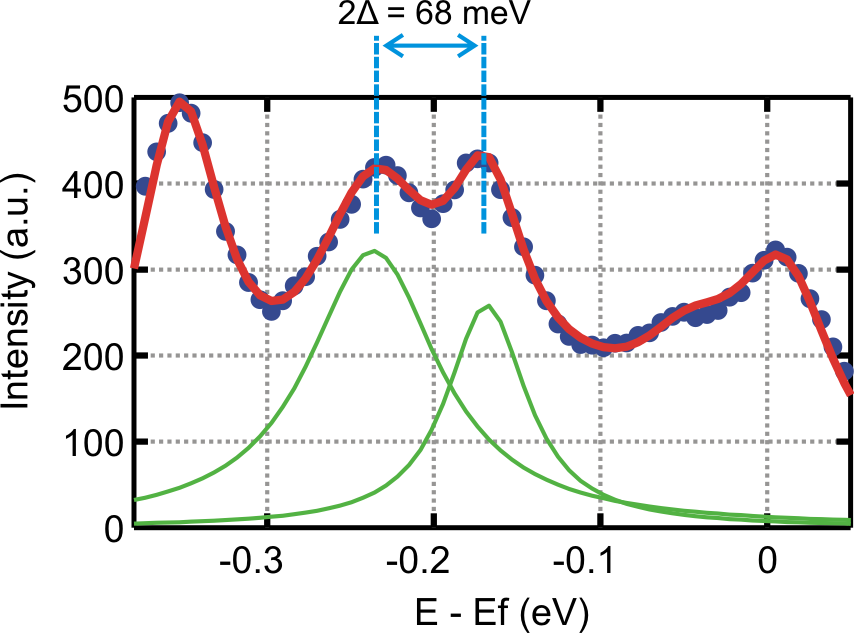
The avoided crossing gaps in Fig. 2c of the main text are determined by taking an Energy Distribution Curve (EDC) at $k_{y}=0.035$ A-1 through the Tr-ARPES spectra obtained at $t=0$ for each pump power. This value of $k_{y}$ corresponds to where the avoided crossing gap is observed. The EDC for the Tr-ARPES spectra in Fig. 2b of the main text is shown in Fig. S1. Each EDC is fitted with multi-peak Lorentz functions. The choice of the peak functions does not affect the obtained gap size in any significant way since we are only interested in the distance between the peaks. The avoided crossing gap is then given by the separation of the two peaks around energy, $E-E_{f}=-0.2$ eV (green peaks in Fig. S1). The resulting gap size for a pump power of $11.5$ mW is then $2\Delta=68$ meV which is in good agreement with the experimental parameters stated in section II as $2\Delta=\beta\omega$ with $\omega=160$ meV and the $\beta=0.42$.

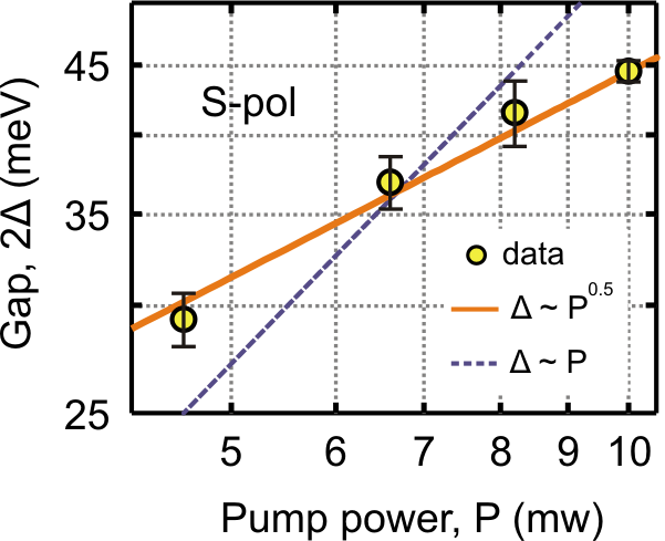
This procedure is also repeated for the case of S-polarized pump and the resulting gap ($2\Delta$) as a function of pump power ($P$) is plotted in Fig. S2 on a log-log plot. Similar to the case of P-polarized pump, $2\Delta$ scales as the square root of the pump power i.e. $2\Delta\propto\sqrt{P}$ in agreement with Floquet-Bloch theory on Dirac systems fregoso13 .

Fig. S 1: Energy Distribution Curve (EDC) at $k_{y}=0.035$ A-1 through the Tr-ARPES spectra in Fig. 2b of the main text. Blue dots indicate the raw data. The red line is a multi-peak Lorentz function best fit to the data. Green peaks correspond to the peaks from which the avoided crossing gap is determined
Refer to caption
Fig. S 2: Avoided crossing gap ($2\Delta$) as a function of incident pump power ($P$) on a log-log plot for S-polarized pump. Error bars represent the 95% confidence interval (2 s.d.) in extracting the gap from the fitting parameters. Power laws ($2\Delta\propto P^{\eta}$) with $\eta=0.5$ (orange trace) and $\eta=1$ (blue trace) are plotted as well to determine the analytical behavior of $2\Delta$ with $P$.
Refer to caption

References

  • (1) J. K. Freericks, H. R. Krishnamurthy, and Th. Pruschke, Phys. Rev. Lett. 102, 136401 (2009).
  • (2) H. Dehghani, T. Oka, and A. Mitra, Phys. Rev. B 90, 195429 (2014).
  • (3) K. I. Seetharam, C.-E. Bardyn, N. H. Lindner, M. S. Rudner, and G. Refael, arXiv:1502.02664 (2015).
  • (4) Y. H. Wang, D. Hsieh, D. Pilon, L. Fu, D. R. Gardner, Y. S. Lee, and N. Gedik, Phys. Rev. Lett. 107, 207602 (2011).
  • (5) S. T. Park, Phys. Rev. A 90, 013420 (2014).
  • (6) Y. H. Wang, H. Steinberg, P. Jarillo-Herrero, N. Gedik, Science 342, 453-457 (2013).
  • (7) B. M. Fregoso, Y. H. Wang, N. Gedik and V. Galitski, Phys. Rev. B 88, 155129 (2013).