Holographic Entanglement Entropy in Time Dependent Gauss-Bonnet Gravity

Abstract

We investigate entanglement entropy in Gauss-Bonnet gravity following a global quench. It is known that in dynamical scenarios the entanglement entropy probe penetrates the apparent horizon. The goal of this work is to study how far behind the horizon can the entanglement probe reach in a Gauss-Bonnet theory. We find that the behavior is quite different depending on the sign of the Gauss-Bonnet coupling $\lambda_{GB}$. For $\lambda_{GB}>0$ the behavior of the probes is just as in Einstein gravity; the probes do not reach the singularity but asymptote to a locus behind the apparent horizon. We calculate the minimum radial position $r_{min}$ reached by the probes and show that for $\lambda_{GB}>0$ they explore less of the spacetime behind the horizon than in Einstein gravity. On the other hand, for $\lambda_{GB}<0$ the results are strikingly different; for early times a new family of solutions appears. These new solutions reach arbitrarily close to the singularity. We calculate the entanglement entropy for the two family of solutions with $\lambda_{GB}<0$ and find that the ones that reach the singularity are the ones of less entanglement entropy. Thus, for $\lambda_{GB}<0$ the holographic entanglement entropy probes further behind the horizon than in Einstein gravity. In fact, for early times it can explore all the way to the singularity.

1 Introduction

The gauge gravity correspondence postulates the equivalence of a gravity theory and a (non-gravitational) quantum field theory at the boundary. For many years this duality has been successfully applied to translate intractable problems in strongly coupled field theories to manageable calculations in the gravity theory. However, it should be possible to use the correspondence in the reverse direction and learn about quantum gravity. In particular, it should be possible to reconstruct the bulk geometry from CFT boundary data. Much work has been done in this direction in the last few years and many puzzles and surprises have been found along the way. The holographic entanglement entropy prescription (HEE) of Ryu and Takayanagi (RT) Ryu:2006bv has played a crucial role in these discoveries. Unfortunately, our understanding of how local bulk information is encoded in the boundary theory is not yet complete.

Since AdS/CFT geometrizes field theory observables relating them to geometrical constructions one can ask how much of the spacetime geometry is accessible to the field theory observables?. This line of work was started in AbajoArrastia:2010yt ,Hubeny:2013gta and developed in Hubeny:2013dea . In AbajoArrastia:2010yt it was shown that spacelike extremal surfaces cannot penetrate the horizon of an asymptotically AdS static black hole but they do penetrate the horizon of a dynamical black hole. It was also noted AbajoArrastia:2010yt Hubeny:2013gta that even though the probes can explore behind the horizon they do not reach arbitrarily close to the singularity. This behavior was later shown to be related to the linear growth of the entanglement entropy as a function of time Liu:2013qca .

A parallel observation in this line of thought comes from the study of HEE in static AdS black holes with compact boundaries. Typically there are two families of extremal surfaces Hubeny:2013gta and we are instructed to choose the one of minimal area as the dual of the entanglement entropy. Which family is the one of minimal area changes depending on where we are in parameter space. The switchover defines a region that the entanglement probe cannot explore and that is dubbed entanglement shadow Freivogel:2014lja .

Given these limitations of the HEE to access the bulk and thus be used to reconstruct it, it is natural to consider that the HEE might not be the right probe. Indeed, other objects (causal holographic information Hubeny:2012wa , entwinement Balasubramanian:2014sra ) have been proposed either as more natural constructions or as being more suited for bulk reconstruction but it is still not clear what is their field theory dual.

In this work we take a different approach; instead of changing the probe we investigate a different gravity theory. The limitations of the HEE to access the bulk that we mentioned above have been studied in Einstein gravity. Thus, it is natural to ask how are these results modified in a higher derivative theory. Such is the aim of the present work. We study holographic entanglement entropy in a dynamical (Vaydia type) scenario in Gauss-Bonnet gravity where the collapse of a null shell results in the formation of an asymptotically AdS black hole.

Previous studies of HEE in this background have been focused on thermalization time of the field theory. Let us note that in the context of AdS/CFT a Gauss-Bonnet background is dual to a theory with central charges $a\neq c$, and the higher derivative terms arise as corrections in the inverse t’Hooft coupling. The values of $\lambda_{GB}$ were known to be constraint to a small window by demanding causality of the field theory Buchel:2009sk ,Hofman:2008ar . These bounds were recently strengthen Camanho:2014apa to show that a consistent holographic theory of quantum gravity with finite $\lambda_{GB}$ would require an infinite tower of higher spin fields. However, it is still possible to treat the higher derivative terms as part of a perturbative expansion of a string or quantum gravity theory. Thus, such bottom-up approach is used in the thermalization time Li:2013cja Zeng:2013mca Zeng:2013fsa and anisotropic plasmas in Gauss-Bonnet Jahnke:2014vwa .

Our interest is not to make contact with a field theory but is more geometric, we want to understand if in higher derivative theories HEE can probe further behind the horizon than in Einstein gravity. In Hubeny:2007xt Hubeny, Rangamani and Takayanagi (HRT) presented a covariant generalization of the holographic entanglement entropy prescription of RT. This proposal enabled the holographic study of time dependent phenomena and out of equilibrium physics. The linear growth of entaglement entropy as a function of time typical of ergodic systems was obtained holographically and the thermalization time explored in scenarios with and without chemical potentialBalasubramanian:2011ur ,Caceres:2012em , Galante:2012pv , Caceres:2012px . The extension of the RT proposal to Gauss-Bonnet theories was initiated in Hung:2011xb and deBoer:2011wk . In Dong:2013qoa ,Camps:2013zua the authors generalized the proposal to arbitrary higher derivatives theories and presented a covariant prescription. Recently, in Headrick:2014cta it was shown that as long as long as the bulk obeys the null energy condition, the covariant prescription for the entanglement entropy HRT is compatible with causality of the field theory. This point was further explored in higher derivative theories in Erdmenger:2014tba .

In this paper we use these results to study HEE in a Gauss-Bonnet black hole formed by collapsing a null shell. We find that for $\lambda_{GB}>0$ the HEE surfaces behave just as in Einstein gravity: they penetrate the horizon but stop at a limiting locus and do not reach the singularity. Furthermore, we calculate the minimum point the geodesics can reach behind the horizon and show that for $\lambda_{GB}>0$ the HEE explores less than HEE in Einstein gravity. For $\lambda_{GB}<0$ the results are strikingly different: at early times the solutions become double valued with one family reaching the singularity and the other not. Given these two families of solutions the prescription instruct us to choose the one of minimal entropy. We find that it is the family that reaches the singularity the one that has minimal entropy. Thus, our results indicate that for $\lambda_{GB}<0$ the holographic entanglement entropy can explore all the way to the singularity. For later times the two families join and again and HEE no longer explores close to the singularity.

This paper is organized as follows: in Section 2 we summarize some known facts of GB gravity and present the background we will use in the rest of the paper. As a warmup we calculate spacelike geodesics in Section 3 ans show that already for spacelike geodesics the curves that reach arbitrarily close to the singularity exist when $\lambda_{GB}<0$. In Section 4 we present the study of HEE in a Vaidya Gauss-Bonnet background for postive and negative coupling, we explain the numerical procedure and present the results. In the last section (Section 5) we present the conclusions and several possible directions that are, in our opinion, interesting to investigate.

2 Gauss-Bonnet gravity

In the framework of the AdS/CFT correspondence, higher derivatives terms are expected to arise as quantum or stringy corrections to the classical action. Thus, it is compelling to consider an effective action where the cosmological constant and Einstein terms are supplemented by curvature corrections. In this section we will gather some well known facts about one particular such theory: Gauss-Bonnet gravity.

Let us consider five dimensional Gauss-Bonnet gravity. This theory is the simplest of Lovelock theories which are known to yield second order equations of motion in spite containing higher derivative terms in the action. They are free of pathologies and are solvable. In fact, many black hole solutions with AdS asymptotics are known Camanho:2011rj .

The action is given by (following the notations in Myers:2012ed , see also deBoer:2011wk )

$$S_{grav}=\frac{1}{16\pi G_{N}}\int d^{5}x\sqrt{-g}\left(R+\frac{12}{L^{2}}+\frac{\lambda_{GB}L^{2}}{2}\mathcal{L}_{(2)}\right),$$ (2.1)

$$\mathcal{L}_{(2)}=R_{\mu\nu\rho\sigma}R^{\mu\nu\rho\sigma}-4R_{\mu\nu}R^{\mu\nu}+R^{2}$$ (2.2)

Here $G_{N}$ denotes the five-dimensional Newtons’s constant, R denotes the Ricci-scalar; the cosmological constant is given by $\Lambda=-12/L^{2}$, where $L$ is some length scale. Varying the action in (2.1), we get the following equation of motion in (2.1)

$$R_{\mu\nu}-\frac{1}{2}g_{\mu\nu}\left(R+\frac{12}{L^{2}}+\frac{\lambda_{GB}L^{2}}{2}\mathcal{L}_{(2)}\right)+\mathcal{H}_{\mu\nu}^{(2)}=0,$$ (2.3)

$$\mathcal{H}_{\mu\nu}^{(2)}=R_{\mu\nu\rho\sigma\lambda_{GB}}R_{\nu}^{\rho\sigma\lambda_{GB}}-2R_{\mu\rho}R_{\nu}^{\rho}-2R_{\mu\rho\nu\sigma}R^{\rho\sigma}+RR_{\mu\nu}.$$ (2.4)

In some sense, the tensor $\mathcal{H}_{\mu\nu}^{(2)}$ can be thought of as an external energy-momentum tensor sourced by the higher derivative terms.

A solution of the equation of motion (2.3) is Cai:2001dz ,

$$ds^{2}=-\frac{L^{2}}{z^{2}}\frac{f(z)}{f_{0}}dv^{2}+\frac{L^{2}}{z^{2}}\left(-\frac{2}{\sqrt{f_{0}}}dzdv+d\bar{x}^{2}\right),$$ (2.5)

$$f(z)=\frac{1}{2\lambda_{GB}}[1-\sqrt{1-4\lambda_{GB}(1-mz^{4})}].$$ (2.6)

The background in (2.5) represents an asymptotically AdS-space black hole solution of Gauss-Bonnet gravity where $L$ is related to the radius of curvature and the event-horizon is located at $z_{eh}=m^{-1/4}$. We have expressed the above solution in Eddington-Finkelstein coordinates, which are defined by

$$dt=dv+\sqrt{f_{0}}\frac{dz}{f(z)}$$ (2.7)

where $t$ is the boundary time. Near the boundary, where $z\rightarrow 0$, $v\rightarrow t$. The constant $f_{0}$ has been chosen such that lim${}_{z\rightarrow 0}f(z)=f_{0}$,

$$f_{0}=\frac{1}{2\lambda_{GB}}\left(1-\sqrt{1-4\lambda_{GB}}\right).$$ (2.8)

we chose to normalize the coordinates in (2.5) such that at the boundary $g_{tt}/g_{xx}|_{z\rightarrow 0}=-1$. In Poincarè patch, the background in (2.5) takes the following form

$$ds^{2}=-\frac{L^{2}}{z^{2}}\frac{f(z)}{f_{0}}dt^{2}+\frac{L^{2}}{z^{2}}d\bar{x}^{2}+\frac{L^{2}}{z^{2}}\frac{dz^{2}}{f(z)}.$$ (2.9)

Note that the parameter $L$ is related to the $AdS$ curvature scale $\tilde{L}$ as $\tilde{L}^{2}=L^{2}/f_{0}$. The temperature of this solution is,

$$T=\frac{m^{1/4}}{\pi L^{2}}\frac{1}{\sqrt{f_{0}}}$$

Note that the event horizon is always located at

$$z_{eh}=m^{-1/4}$$ (2.11)

regardless of the value of $\lambda_{GB}$. The curvature singularity that occurs at $z=\infty$ for $\lambda_{GB}\geq 0$ is shifted to a finite radial position,

$$z_{s}=\frac{1}{\sqrt{2}m^{1/4}\lambda_{GB}^{1/4}}(-1+4\lambda_{GB})^{1/4}$$ (2.12)

for $\lambda_{GB}<0$.

Finally, througout this paper we will work with very small values of the Gauss-Bonnet coupling, $\lambda_{GB}=\pm 0.05$ as representativs of positive and negative Gauss-Bonnet couplings.

2.1 Time dependent background

We will now us discuss a time-dependent generalization of the background in (2.5). In order to do so, we need to couple the action $S_{grav}$ in (2.1) with an external source term $S_{ext}$ to yield

$$S=S_{grav}+\kappa S_{ext},$$

where $\kappa$ is some coupling which we do not specify here. A simple solution of the following form can be obtained

$$ds^{2}=-\frac{L^{2}}{z^{2}}\frac{f(z,v)}{f_{0}}dv^{2}+\frac{L^{2}}{z^{2}}\left(-\frac{2}{\sqrt{f_{0}}}dzdv+d{\bar{x}}^{2}\right),\qquad f_{0}=\frac{1}{2\lambda_{GB}}(1-\sqrt{1-4\lambda_{GB}}),$$ (2.13)

$$f(z,v)=\frac{1}{2\lambda_{GB}}\left[1-\sqrt{1-4\lambda_{GB}(1-m(v)z^{4})}\right].$$ (2.14)

Here $m(v)$ is a function that is hitherto undetermined. It is straightforward to check that the external source must yield the following energy-momentum tensor

$$(16\pi G_{N})\kappa T^{ext}_{\mu\nu}=\frac{3}{2}z^{3}\frac{dm}{dv}\delta_{\mu v}\delta_{\nu v}.$$ (2.15)

Thus a null energy condition on the external energy momentum tensor will give the condition $m^{\prime}(v)\geq 0$. Null energy condition in the bulk is related to strong subadditivity in the boundaryCallan:2012ip ,Caceres:2013dma . We want to preserve both of them so we will choose a profile that satisfies $m^{\prime}(v)\geq 0$ . Since this is a time-dependent geometry we need to identify the apparent horizon.

A trapped surface $T$ is a co-dimension two spacelike submanifold such that the expansion of both “ingoing” and “outgoing” future directed null geodesics orthogonal to $T$ is everywhere negative. The boundary of the trapped surfaces is the apparent horizon.

In what follows, we will closely follow Figueras:2009iu . For the background in (2.13) the vectors tangent to the ingoing and outgoing null geodesics are given by

$$l_{-}=-\partial_{z}\ ,\quad l_{+}=-\frac{z^{2}}{L^{2}}\partial_{v}+\frac{z^{2}}{2L^{2}}f\sqrt{f_{0}}\partial_{z}\$$ (2.16)

such that

$$l_{-}\cdot l_{-}=0\ ,\quad l_{+}\cdot l_{+}=0\ ,\quad l_{-}\cdot l_{+}=-1\ .$$ (2.17)

Now the volume element of the co-dimension two spacelike surface (orthogonal to the above null geodesics) is given by

$$\Sigma=\left(\frac{L}{z}\right)^{3}\ .$$ (2.18)

The expansions are defined to be

$$\theta_{\pm}={\cal L}_{\pm}\log\Sigma=l_{\pm}^{\mu}\partial_{\mu}\left(\log\Sigma\right)\ ,$$ (2.19)

where ${\cal L}_{\pm}$ denotes the Lie derivatives along the null vectors $l_{\pm}$. The apparent horizon is then obtained by solving the equation $\Theta=0$, where $\Theta=\theta_{+}\theta_{-}$ is the invariant quantity. In this case we find

$$\Theta=\frac{9}{2L^{2}}f(z_{ah},v)=0$$ (2.20)

gives the location of the apparent horizon,

$$z_{ah}=m(v)^{-1/4}$$ (2.21)

The event horizon, on the other hand, is a null surface in the geometry (2.13),

$$\mathcal{N}=z-z_{eh}(v),\qquad\qquad G^{\mu\nu}\partial_{\mu}\mathcal{N}\partial_{\nu}\mathcal{N}=0,$$ (2.22)

which gives the evolution of the event horizon,

$$z_{eh}^{\prime}(v)=-\frac{1}{2\sqrt{f_{0}}}f(z_{eh},v).$$ (2.23)

It is clear form (2.20) that the position of the apparent horizon does not depend on $\lambda_{GB}$. However, the position of the event horizon does albeit mildly (see Figure 1)

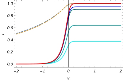
Figure 1: The dashed lines are the event horizons for $\lambda_{GB}=0.05,\ -0.05$ The red line is the apparent horizon which is independent of $\lambda_{GB}$ and the other lines are the singularity for different values of $\lambda_{GB}=-.0.005,\ -0.05,\ -.5,\ -1.$ from bottom to top respectively.

Our goal in the next sections is to study non-local probes in (2.13) that evolves between a vacuum AdS geometry with radius and an asymptotically AdS black hole solution of Gauss Bonnet action (2.1). We will be particularly interested in comparing how far behind the apparent horizon the different probes can reach. Our main interest is the behavior of the entanglement entropy, Section 4. However, we will first analyze spacelike geodesics which already illustrate some novel features also present in the entanglement entropy.

3 Spacelike geodesics

To find spacelike geodesics in the background (2.13) we extremize the following Lagrangian

$$\mathcal{L}=\frac{1}{z(x)}\sqrt{f_{0}-f(z,v)v^{\prime}(x)^{2}-2\sqrt{f_{0}}v^{\prime}(x)z^{\prime}(x)}$$ (3.24)

The equations of motion are

$$z^{\prime\prime}(x)=\mathcal{Z}[v(x),z(x)]$$

$$v^{\prime\prime}(x)=\mathcal{V}[v(x),z(x)]$$ (3.25)

The equations of motion will be solved subject to boundary conditions

$$z(l/2)=z(-l/2)=z_{0}\qquad\qquad\textrm{ and}\qquad\qquad z^{\prime}(0)=v^{\prime}(0)=0$$

where $l/2$ denotes the distance in the boundary and $z_{0}$ is the IR cutoff. The Lagrangian (3.24) does not depend explicitly on $x$, the corresponding conserved quantity is,

$$\frac{1}{z(x)^{2}\mathcal{L}}=C_{1}.$$ (3.26)

We will be working with a thin shell, $M(v)=\frac{1}{2}(1+\tanh(v/v_{0}))$ with $v_{0}=0.01$. As the parameter $v_{0}$ goes to zero, this function approximates a step function. Thus, in the limit $v_{0}\rightarrow 0$ the spacetime is given by the gluing of two static geometries. Let us pause and, to gain some intuition, briefly study the behavior of geodesics in static Gauss Bonnet spaces.

If $M(v)=m$, $v$ is a cyclic variable and its associated momentum is conserved,

$$\frac{-f(z)v^{\prime}(x)-\sqrt{f_{0}}z^{\prime}(x)}{z(x)^{2}\mathcal{L}}=C_{2}$$ (3.27)

Thus, in the static case we have two conserved quantities (3.26) and (3.27). It is instructive to find the effective potential in this case since it will illustrate the differences for $\lambda_{GB}>0$ and $\lambda_{GB}<0$ that will persist in the dynamic case. Solving (3.26) for $v^{\prime}(x)$ and substituting in (3.27) we get

$$z^{\prime}(x)^{2}=E^{2}-V_{eff}$$ (3.28)

where

$$V_{eff} =f(z,\lambda_{GB})(1-\frac{{\cal J}^{2}}{z^{2}}).\$$ (3.29)

 

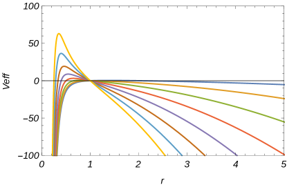
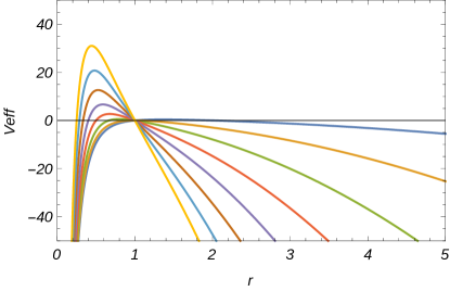
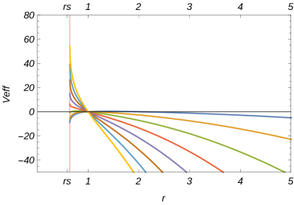
Figure 2: Effective potential $V_{eff}(r)$ for $m=1$ and different values of ${\cal J}$. Left panel : $\lambda_{GB}=.05$.  Right panel: $\lambda_{GB}=-0.05.$ In the lower panel we have included the $SAdS$ case for comparison.

For convenience we have redefined the constants as $E=\frac{C_{2}}{C_{1}}\sqrt{f_{0}(\lambda_{GB})}$ and ${\cal J}=\frac{1}{C_{1}}$. In Figure (2) we plot $V_{eff}$ for different values of $C_{1}$ as a function of $r=1/z$. Note the different behavior of the potential for $\lambda_{GB}>0$ and $\lambda_{GB}<0$. For $\lambda_{GB}>0$ the potential is similar to the Schwarzchild $AdS_{5}$ ($SAdS_{5}$); it reaches a maximum for some value of $0<r<rh$ and the value of the maximum grows with large ${\cal J}$. The growth of this maximum becomes less pronounced as we increase $\lambda_{GB}$. For $\lambda_{GB}<0$ the potential is qualitatively different. For small values of ${\cal J}$ it is a concave function that reaches its maximum at some $r_{s}<r<r_{h}$ similar to the positive $\lambda_{GB}$ case. However, for large ${\cal J}$ the concavity of the potential changes and reaches its maximum at the singularity $r_{s}$. We identify the critical value of ${\cal J}$ at which this change occurs,

$${\cal J}_{crit}\sim\frac{1}{2\sqrt{-\lambda_{GB}}(1+2\lambda_{GB})}.$$ (3.30)

The existence of this different regimes in the case of negative $\lambda_{GB}$ is clearly asociated with the fact that the singularity has shifted from $r=0$ to $r_{s}^{-1}=\frac{1}{\sqrt{2}m^{1/4}\lambda_{GB}^{1/4}}(-1+4\lambda_{GB})^{1/4}$. This different behavior of $V_{eff}$ for $\lambda_{GB}<0$ and $\lambda_{GB}>0$ will be reflected in the time dependent case.

Now we are ready to proceed with the time dependent case with $M(v)$ in (2.13) given by $M(v)=\frac{1}{2}(1+\tanh{\frac{v}{v_{0}}})$. We want to solve the differential equations 3 subject to the following boundary conditions

$$z(0)=z_{*},\quad z^{\prime}(0)=0,\quad v(0)=v_{*},\quad v^{\prime}(0)=0$$

So far $z_{*}$ and $v_{*}$ are two free parameters that generate the numerical solutions for $z(x)$ and $v(x)$. Once a solution is obtained the boundary data can be read off,

$$z(l/2)=z_{0}\qquad\qquad v(l/2)=t_{b}$$

. Note that the numerically nontrivial part is to look for appropriate parameters $(z_{*},v_{*})$ such that the IR cutoff $z_{0}$ is a small number . We will expand on the details of the numerical procedure in section (4.1) when we deal with the HEE probes that is our main objective.

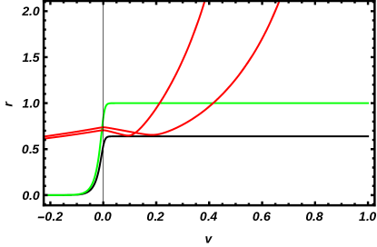
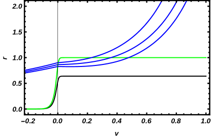
Figure 3: Representative geodesics for negative $\lambda_{GB}$. Left panel: the new family of solutions that reach the singularity. Right panel: the standard solutions that asymptote to a critical surface and do not reach the singularity.

We solve the equations of motion and look for geodesics that cross the horizon and are anchored at the boundary. We find that the case of negative $\lambda_{GB}$ presents some new features. There are geodesics that, as in SAdS-Vaidya, cross the horizon but do not reach the singularity and asymptote to a limiting surface. But there is also – for some range of parameters– a new family of boundary anchored geodesics that do reach arbitrarily close to the singularity. It is remarkable that this strikingly different behavior depends crucially on the sign of $\lambda_{GB}$ and is present even for such a small value of the coupling as $\lambda_{GB}=-0.05$. In Figure (3) we plot some representative solutions.

4 Entanglement Entropy

The proposal for computing entanglement entropy is modified acording to the formula obtained in deBoer:2011wk Hung:2011xb

$$S_{EE}=\frac{1}{4G_{N}}\int_{\Sigma}d^{3}\xi\sqrt{\gamma}(1+\lambda_{GB}L^{2}R_{\Sigma})+\frac{1}{2G_{N}}\int_{\partial\Sigma}d^{2}\xi\sqrt{h}K,$$ (4.31)

where $\Sigma$ denotes the three dimensional surface anchored at the two dimensional boundary of the region A; $\xi$ denotes the worldvolume coordinates on the surface and $h$ denotes the induced metric on this surface. The quantity $R_{\Sigma}$ denotes the Ricci scalar constructed from the induced metric on $\Sigma$ and the last term in (4.31) is the Gibbons-Hawking boundary term that one needs to introduce to have well a defined variational problem. The proposal (4.31) was initially put forward for time independent situations. In Dong:2013qoa ,Camps:2013zua the authors generalize the proposal of deBoer:2011wk , Hung:2011xb and presented a covariant prescription valid for more general theories of higher derivatives.

Throughout this paper we will study the “rectangular strip” in the backgrounds (2.13). Assuming translational invariance in two of the directions we can parametrize the extremal area surface by the third coordinate, $x$, and we have ${z(x),v(x)}$ . We denote the width of the rectangular strip $\ell$, that is $\frac{\ell}{2}<x<\frac{\ell}{2}$. The induced metric on the co-dimension two surface is given by

$$ds^{2}=\frac{L^{2}}{z^{2}}(dx_{2}^{2}+dx_{3}^{2})+\frac{L^{2}}{z^{2}}\left(1-\frac{f}{f_{0}}v^{\prime 2}-\frac{2}{\sqrt{f_{0}}}v^{\prime}z^{\prime}\right)dx^{2},$$ (4.32)

where once more we have ${}^{\prime}\equiv d/dx$. This now gives

$$\sqrt{\gamma}=\frac{L^{3}}{\sqrt{f_{0}}}\frac{1}{z^{3}}\left(f_{0}-fv^{\prime 2}-2\sqrt{f_{0}}v^{\prime}z^{\prime}\right)^{1/2}\ ,$$ (4.33)

$$\lambda_{GB}L^{2}\sqrt{\gamma}R_{\Sigma}=(2L^{3}\lambda_{GB}\sqrt{f_{0}})\frac{z^{\prime 2}}{z^{3}\left(f_{0}-fv^{\prime 2}-2\sqrt{f_{0}}v^{\prime}z^{\prime}\right)^{1/2}}+\frac{dF}{dz}\ ,$$ (4.34)

where

$$F(x)=(4L^{3}\lambda_{GB}\sqrt{f_{0}})\frac{z^{\prime}}{z^{2}\left(f_{0}-fv^{\prime 2}-2\sqrt{f_{0}}v^{\prime}z^{\prime}\right)^{1/2}}$$ (4.35)

Clearly, the total derivative term will not contribute to the equations of motion. Furthermore, the $dF/dx$ term is exactly cancelled by the Gibbons-Hawking term . Thus, the effective action that needs to be extremized is given

$$S_{eff}=\frac{L^{3}}{4G_{N}\sqrt{f_{0}}}\int\frac{dz}{z^{3}}\left[\left(f_{0}-fv^{\prime 2}-2\sqrt{f_{0}}v^{\prime}z^{\prime}\right)^{1/2}+\frac{2\lambda_{GB}f_{0}z^{\prime 2}}{\left(f_{0}-fv^{\prime 2}-2\sqrt{f_{0}}v^{\prime}z^{\prime}\right)^{1/2}}\right].$$ (4.36)

The equations of motion derived from (4.36) are,

$$z^{\prime\prime} =\frac{F_{z}(z,z^{\prime},v,v^{\prime})}{G(z,z^{\prime},v,v^{\prime})}$$ (4.37)

$$v^{\prime\prime} =\frac{F_{v}(z,z^{\prime},v,v^{\prime})}{G(z,z^{\prime},v,v^{\prime})}$$ (4.38)

where we are not writing explicitly the $x$ dependence in $z(x)$, $v(x)$ and ^′ denotes derivative with respect to $x$.

$$F_{z} =\sqrt{f_{0}}f(z,v)\bigg{[}\sqrt{f_{0}}v^{\prime 2}\left[\left(6\lambda_{GB}zz^{\prime 2}-z\right)\partial_{z}f(z,v)-24z^{\prime 2}\right]$$ (4.39)

$$+4zv^{\prime 3}z^{\prime}\partial_{z}f(z,v)+zv^{\prime 4}\partial_{v}f(z,v)+6f_{0}^{3/2}\left(2\lambda_{GB}z^{\prime 2}-1\right)-24f_{0}v^{\prime}z^{\prime}\left(\lambda_{GB}z^{\prime 2}-1\right)\bigg{]}$$

$$+v^{\prime 2}f(z,v)^{2}\left[zv^{\prime 2}f^{(1,0)}(z,v)-24\sqrt{f_{0}}v^{\prime}z^{\prime}-12f_{0}\left(\lambda_{GB}z^{\prime 2}-1\right)\right]$$

$$+f_{0}zv^{\prime}\big{[}v^{\prime}\partial_{v}f(z,v)+2z^{\prime}\partial_{z}f(z,v)\big{]}\left[6\lambda_{GB}\sqrt{f_{0}}z^{\prime 2}-\sqrt{f_{0}}+2v^{\prime}z^{\prime}\right]-6v^{\prime 4}f(z,v)^{3}$$

$$F_{v} =zv^{\prime}\partial_{z}f(z,v)\bigg{[}-2\sqrt{f_{0}}z^{\prime}\left[v^{\prime 2}-4\lambda_{GB}v^{\prime 2}f(z,v)+4f_{0}\lambda_{GB}\right]$$ (4.40)

$$+v^{\prime}\left[f_{0}-v^{\prime 2}f(z,v)\right]+10f_{0}\lambda_{GB}v^{\prime}z^{\prime 2}\bigg{]}-2\left[f_{0}-v^{\prime}\left(v^{\prime}f(z,v)+2\sqrt{f_{0}}z^{\prime}\right)\right]$$

$$\times\left[2\sqrt{f_{0}}\left(\lambda_{GB}zv^{\prime 2}\partial_{v}f(z,v)+3z^{\prime}\left(\sqrt{f_{0}}\lambda_{GB}z^{\prime}+v^{\prime}\right)\right)+3v^{\prime 2}f(z,v)-3f_{0}\right]$$

$$G=2\sqrt{f_{0}}z\left[(4\lambda_{GB}f(z,v)+1)\left(v^{\prime 2}(-f(z,v))-2\sqrt{f_{0}}v^{\prime}z^{\prime}+f_{0}\right)-6f_{0}\lambda_{GB}z^{\prime 2}\right]$$ (4.41)

We will solve these equations of motion subject to the initial conditions,

$$z(0)=z_{*},\qquad\qquad z^{\prime}(0)=0$$ (4.42)

and,

$$v(0)=v_{*},\qquad\qquad v^{\prime}(0)=0.$$ (4.43)

Thus a particular solution is labeled by $(z_{*},v_{*})$. We are interested in $(z_{*},v_{*})$that produce surfaces anchored at the boundary. We also want relate this constants to boundary quantities $\ell$ and $t_{b}$. The numerical procedure used to do this is explained below.

4.1 Numerical procedure

In order to solve the motion equation numerically, we employ the Dormand-Prince method Dormand , which is an explicit method to solve systems of differential equations. This method uses six evaluations to compute the fourth and fifth order solutions and employ them to estimate the relative error, once determined the error, the program uses an automatic step adjusting procedure. In the present work we used the C language implementation of the Dormand- Prince method provided by Dop853 . Notice that the condition that the homology condition, in this case equivalent to demanding that the surface is anchored at the boundary, is not included a priori on the system of differential equations, they need to be considered during the selection of initial conditions. Because the solutions diverges at the boundary, it is not possible to set the initial conditions there. However, since we know that at least in two points $z\rightarrow 0$, there is a maximum point $z_{*}$ , by translational invariance we may set

$$z(0)=z_{*},\qquad\qquad z^{\prime}(0)=0$$ (4.44)

this completely fixes the initial conditions for $z(x)$. In a similar way we impose the initial conditions for $v(x)$ to be

$$v(0)=v,\qquad\qquad v^{\prime}(0)=0.$$ (4.45)

Then we may parametrize the set of all the solutions by $(z_{*},v_{*})$. We want to relate the parameters $(z_{*},v_{*})$ with the parameters at the bound ary $(\ell,t_{b})$, to do so we notice that, by symmetry, $z(\pm\ell/2)=0$ and $v(\pm\ell/2)=t_{b}$. These equations stablish a relation between the two set of parameters, however it is not possible to solve them in general. Instead of that we proceed to scan de parameter space $(z_{*},v_{*})$ in the region $z_{*}\in(0,10]$ y $v_{*}\in[-10,10]$ using a grid of$600\times 600$ or $800\times 800$ over applied over different subregions. The grid size and the region to be explore were chosen to maxi- mize the number of curves satisfying the homology condition and crossing the apparent horizon. In order to solve the system of differential equation over the grid in a more efficient way we divide the process into 10 or 20 parallel processors. Once obtained a list of acceptable initial conditions, those which are anchored at the boundary, we proceed to choose those solutions which satisfied any required boundary conditions, i.e. $\ell$ and $t_{b}$ , the precision with which those values are determined depends on the grid step, for the present work we keep a precision in the boundary condition determination of $\pm 0.05$ After solving the system of equations and properly imposing the homology condition we now need to evaluate the entanglement entropy function on-shell, this procedure needs to be done numerically as well.

We need to be careful due the divergent behaviour of the integral at the boundary. For the static cases this is solved by using the conserved quantity to write the integral in terms of $z$, imposing a UV cut-off $z_{0}$ and subtracting the divergent contribution. In static Gauss-Bonnet backgrounds the divergent contribution can be computed in a standard way in the static limit by subtracting the vacuum contribution. However, it will depend on $\lambda_{GB}$. This stems from the fact that vacuum Gauss-Bonnet is an AdS space but with a $\lambda_{GB}$ dependent radius.

In the dynamic case that procedure cannot be employed since we have no conserved quantities, although the divergent contribution to the integral is the same as in the static case, the problem arises when determining the proper way to impose a UV cut-off in a consistent way, this is which match with the static cut-off in the asymptotic limit. Instead of directly impose a cut in the x interval, we employ the numerical integration algorithm itself, imposing a desire precision and a maximal number of step reduction, once reached those values the integral is declared as divergent and the integration finished at that value of x.

4.2 Results

We carried out a numerical study of HEE in backgrounds with $\lambda_{GB}=0.05$ and $\lambda_{GB}=-.05$ as representatives of theories with positive and negative $\lambda_{GB}$. We find that while for positive $\lambda_{GB}$ the behavior of the extremal surface solution of (4.37) is qualitatively similar to the case of Einstein gravity, for negative $\lambda_{GB}$ it is strinkingly different. We summarize our results below:

• For $\lambda_{GB}<0$ and for early times and $\ell\geq 2.5$ a new family of solution appears. That is, for a given $t_{b}$ and $\ell$ two solutions are possible: one that behaves just like $\lambda_{GB}>0$, we denote this family $\mathcal{M}^{0}$, and one that probes arbitrarily close to the singularity, $\mathcal{M}^{S}$, Fig.(4).

  

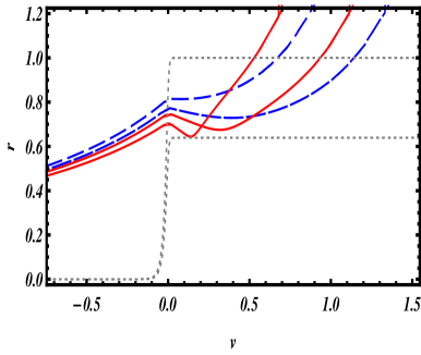
  Figure 4: Representatives of the two families of minimal surfaces for negative Gauss Bonnet coupling, $\lambda_{GB}=-.05$ . The family $\mathcal{M}^{S}$ , red curves, contains surfaces that probe arbitrarily close to the singularity. The family $\mathcal{M}^{0}$ , dashed curves, is very similar to the $SAdS$ and $\lambda_{GB}>0$, they explore behind the horizon but do not reach the singularity.

• We studied the minima, $r_{min}$, reached by the extremal surfaces and present the results in Fig. (5). We can see that for early times the family $\mathcal{M}^{S}$ probes arbitrarily close to the singularity $r_{min}^{S}\sim r_{s}$, where $r_{s}^{-1}$ is defined in (2.12). As time increases $r_{min}^{S}$ becomes larger and for later times the minima converge such that $r_{min}^{S}\sim r_{min}^{0}\sim r_{min}^{\lambda_{GB}>0}\sim r_{min}^{SAdS}$.

  

  

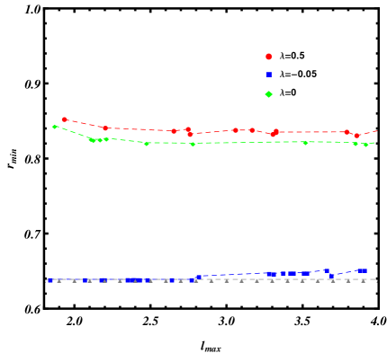
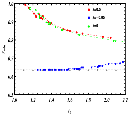
  Figure 5: The minimum point reached by a given entanglement entropy surface for $SAdS$, green, $\lambda_{GB}>0$, red, and $\lambda_{GB}<0$, blue. Top panel: $r_{min}$ as function of the boundary separation $\ell$. Bottom panel: $r_{min}$ as function of the boundary time $t_{b}$.

• We evaluate the functional in these solutions and find that the one that penetrates deeper behind the horizon, close to the singularity, is the one that represents the entanglement entropy Fig.(6).

• As a check of our solutions we calculated entanglement entropy as a function of $\ell$. The concavity of this curve is associated with the validity of strong subadditivity Callan:2012ip , Allais:2011ys . We find that our solutions obey SSA as expected.

• The $\lambda_{GB}>0$ case is very similar to $SAdS$, the extremal surfaces penetrate the horizon but only up to a limiting surface. When we compare the minima we find that for $\lambda_{GB}>0$ the extremal surfaces explore less than in the $AdS$ geometry Fig.(5).

• As mention in section (4) the prescription of for the entanglement entropy in a Gauss Bonnet theory is not just a minimal volume as in Einstein gravity. It is natural to ask if the new effects seen here for $\lambda_{GB}<0$ are due to the extra term in the functional or if they are already present in a minimal volume. In order to elucidate this point we calculate the minimal volume for strip regions in an asymptotically AdS Gauss Bonnet black hole (2.13). We find that the minimal volumes also reach close to the singularity in the case of $\lambda_{GB}<0$. We present the corresponding figures in Appendix (C).

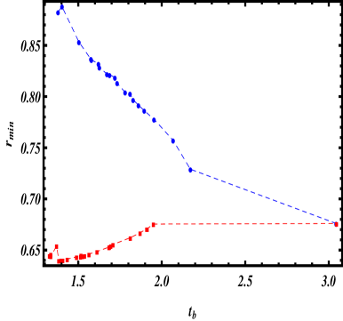
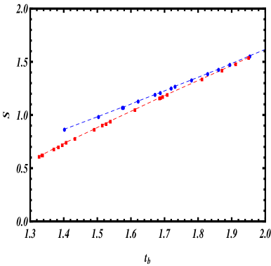
Figure 6: Left panel: minima for the two families of extremal surfaces $\mathcal{M}^{S}$, red and $\mathcal{M}^{0}$, blue. Right panel: Their correponding entanglement entropy .

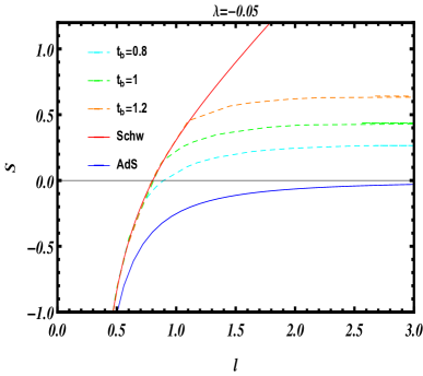
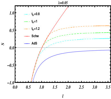
Figure 7: Entanglement entropy as a function of $\ell$ for $\lambda_{GB}=-.05$ (left panel) and $\lambda_{GB}=.05$ (right panel)

5 Conclusions and future directions

The main motivation of this work is a simple question, how far behind the horizon does the HEE probe reach in Gauss-Bonnet theories?. Much is known about the similar question in Einstein gravity but previous studies in Gauss-Bonnet have focused in finding the thermalization time and not in the reach of the probes. In the AdS/CFT context higher derivative theories are interesting because they are dual to field theories with corrections in $1/\sqrt{g_{YM}N}$. We chose Gauss-Bonnet as example of a higher derivative theory because of its solvability; there are black hole solutions known analytically. We take Gauss-Bonnet as a toy model where to learn features of holographic entanglement entropy in a higher derivative theory and not as a dual of a particular field theory. As a warmup we studied geodesics in a Vaidya Gauss-Bonnet background. When $\lambda_{GB}$ is positive there are no surprises, the holographic probes behaves as in Einstein gravity. Namely, they penetrate behind the apparent horizon but not arbitrarily close to the singularity; they asymptote to a certain critical surface. A different and novel behavior appears when we consider $\lambda_{GB}<0$: the solutions become double valued. A new family of solutions that can reach arbitrarily close to the singularity appears. We observe the same behavior in minimal volume surfaces. However, in a 5 dimensional bulk these objects are purely geometric, they are not dual to any field theory observable.

Unlike in Einstein gravity, the holographic entanglement entropy prescription for higher derivative theories Camps:2013zua ,Dong:2013qoa is not only a minimal area but includes an extra term involving the extrinsic curvature. We study the entanglement entropy in a Vaidya Gauss-Bonnet background and quantify how much behind the horizon the probes reach, $r_{min}$ , and find that for $\lambda_{GB}>0$ the probes explore less than in Einstein gravity, i.e $r_{min}^{GB}>r_{min}^{Einstein}$.

For $\lambda_{GB}<0$ we find two family of solutions: one that behaves very similar to Einstein gravity and a new one that reaches arbitrarily close to the singularity. Having two solutions the HRT prescription instruct us to choose the one of minimal entropy. We find that the surfaces reaching the singularity are the ones of minimal entropy. Thus, for $\lambda_{GB}<0$ the holographic entanglement entropy can probe all the way to the singularity. This is the main result of the present work. As a check of our solutions we verify the concavity of $S(l)$ impliying that SSA is respected.

Let us point some open problems and future directions related to the present work;

• Lionhearted effort: Because of its time dependent nature, the problem studied here is numerically intensive. We have concentrated in $\lambda_{GB}=0.05$ and $\lambda_{GB}=-0.05$ as representatives of positive and negative couplings. A complete analysis scanning over a range of values of $\lambda_{GB}$ would certainly be desirable and interesting and might uncover interesting physics as $\lambda_{GB}$ becomes larger. In particular, the novel solutions discovered here for negative $\lambda_{GB}$ (the ones that can reach the singularity) exist only for a very short time after the probe has crossed the shell. It is natural to think that as $\lambda_{GB}$ grows more negative these type of solutions will exist for a larger time. Or it could be that the opposite is true, that for larger negative $\lambda_{GB}$ these solutions cease to exist. The only way to answer these questions is a full numerical analysis over the $\lambda_{GB}$ parameter space.

• An inmediate generalization of the present work would be to study spacetimes of dimensions higher than 5 and boundary regions other than the strip.

• It would be interesting to ask the same question investigated here in other higher derivative theories like more general Lovelock theories where many black hole solutions are known Camanho:2011rj . Also, thermalization in hyperscaling violating backgrounds was investigated in Fonda:2014ula ,Alishahiha:2014cwa and higher derivative corrections in Bueno:2014oua ,Knodel:2013fua . Thus, extending the present work to hyperscaling violating geometries seems a viable and interesting endeavor.

• We have studied entanglement entropy in a time dependent Gauss-Bonnet background in Poincare patch. It the static case, it is known that novel features of the entanglement entropy appear when considering compact spaces Hubeny:2013gta . Thus, extending the present work to spherically symmetric spaces might also uncover some new phenomena sensitive to the sign of the Gauss-Bonnet coupling $\lambda_{GB}$.

• In the same spirit of understanding how much of the bulk does the HEE probes, it would be interesting to consider an asymptotically global AdS static black hole in Gauss-Bonnet gravity and study the entanglement shadow. We expect that entanglement shadow will increase or decrease (as compared to Einstein gravity) depending on the sign of $\lambda_{GB}$.

• It would be interesting to perform as similar study with different holographic probes like the causal holographic information. The acausality of the boundary theory for finite $\lambda_{GB}$ might be reflected in some particular behavior of the causal holographic information surface $\chi_{A}$.

• In Bhattacharyya:2009uu a formalism was developed to study black hole formation in a weak field limit. As shown in Caceres:2014pda some of the interesting physics discovered using the Vaidya model for charged black holes Caceres:2012em can be captured in the weak field approach. Although valid only after a certain time after collapse, the advantage of the perturbative approach is that it is numerically simpler. Thus, it would be interesting to investigate scalar collapse in a Gauss Bonnet theory in the weak field limit and see if some of the results presented here can be also obtained in that framework.

We hope to return to some of these problems in the near future.

Appendix A Gibbons-Hawking term

In this appendix we provide details of the calculation of the boundary term,

$$S_{GH}=\oint_{\partial\Sigma}\sqrt{h}\mathcal{K}.$$

To fix notation, recall that the integral A is over the boundary of the codimension 2 surface $\Sigma$ with induced metric $\gamma$, $h$ is the metric induced at the boundary and $\mathcal{K}$ the trace of the extrinsic curvature of $\Sigma$.

As we saw in 4.32, the metric induced in the co-dimension two surface is

$$\gamma_{ab}dx^{a}dx^{b}=\frac{L^{2}}{z^{2}}\left(1-\frac{f}{f_{0}}v^{\prime 2}-\frac{2}{\sqrt{f_{0}}}v^{\prime}z^{\prime}\right)dx^{2}+\frac{L^{2}}{z^{2}}(dx_{2}^{2}+dx_{3}^{2}),$$ (1.46)

The unit norm vector perpendicular to the boundary is clearly in the $x$ direction,

$$\eta=(\frac{L}{z}\sqrt{\left(1-\frac{f}{f_{0}}v^{\prime 2}-\frac{2}{\sqrt{f_{0}}}v^{\prime}z^{\prime}\right)},0,0)$$

the trace of the extrinsic curvature is then

$$\mathcal{K}=\gamma^{ab}\nabla_{a}\eta_{b}=2\frac{z^{\prime}\sqrt{f_{0}}}{L\sqrt{f_{0}+fv^{\prime 2}-2\sqrt{f_{0}}v^{\prime}z^{\prime}}}$$

Now, the determinant of the metric induced at the boundary is simply $\frac{L^{2}}{z^{2}}$. Thus we have

$$S_{GH}=\oint_{\partial\gamma}dx_{2}dx_{3}2L\frac{z^{\prime}\sqrt{f_{0}}}{z^{2}\sqrt{f_{0}+fv^{\prime 2}-2\sqrt{f_{0}}v^{\prime}z^{\prime}}}$$

which exactly cancels the term $\int\frac{dF}{dx}$ in 4.34.

Appendix B Equations of motion

B.1 Minimal volume

$$\mathcal{L}=\frac{1}{z^{3}}\sqrt{f_{0}-f(z,v)v^{\prime 2}-2\sqrt{f_{0}}v^{\prime}z^{\prime}}$$ (2.47)

The equations of motion are,

$$z^{\prime\prime} =\frac{F_{z}(z,z^{\prime},v,v^{\prime})}{G(z,z^{\prime},v,v^{\prime})}$$ (2.48)

$$v^{\prime\prime} =\frac{F_{v}(z,z^{\prime},v,v^{\prime})}{G(z,z^{\prime},v,v^{\prime})}$$ (2.49)

where we are not writing explicitly the $x$ dependence in $z(x)$, $v(x)$ and ^′ denotes derivative with respect to $x$.

$$F_{z} =-(6f(z,v)^{2}v^{\prime 2}+f(z,v)(6f_{0}+12\sqrt{f_{0}}v^{\prime}z^{\prime}+zv^{\prime 2}\partial_{z}f(z,v))$$ (2.50)

$$\sqrt{f_{0}}zv^{\prime}(v^{\prime}\partial_{v}f(z,v)+2z^{\prime}\partial_{z}f(z,v)))$$

$$F_{v} =6f_{0}-12\sqrt{f_{0}}v^{\prime}z^{\prime}+v^{\prime 2}(-6f(z,v)+z\partial_{z}f(z,v))$$ (2.51)

$$G=2\sqrt{f_{0}}z$$ (2.52)

B.2 Geodesics

$$\mathcal{L}=\frac{1}{z}\sqrt{f_{0}-f(z,v)v^{\prime 2}-2\sqrt{f_{0}}v^{\prime}z^{\prime}}$$ (2.53)

The equations of motion are,

$$z^{\prime\prime} =\frac{F_{z}(z,z^{\prime},v,v^{\prime})}{G(z,z^{\prime},v,v^{\prime})}$$ (2.54)

$$v^{\prime\prime} =\frac{F_{v}(z,z^{\prime},v,v^{\prime})}{G(z,z^{\prime},v,v^{\prime})}$$ (2.55)

$$F_{z} =-(2f(z,v)^{2}v^{\prime 2}+f(z,v)(2f_{0}+4\sqrt{f_{0}}v^{\prime}z^{\prime}+zv^{\prime 2}\partial_{z}f(z,v))$$ (2.56)

$$\sqrt{f_{0}}zv^{\prime}(v^{\prime}\partial_{v}f(z,v)+2z^{\prime}\partial_{z}f(z,v)))$$

$$F_{v} =2f_{0}-4\sqrt{f_{0}}v^{\prime}z^{\prime}+v^{\prime 2}(-2f(z,v)+z\partial_{z}f(z,v))$$ (2.57)

$$G=2\sqrt{f_{0}}z$$ (2.58)

Appendix C Minimal Volume results

In order to understand if the effects found for $\lambda_{GB}$ in the entanglement entropy are due to the correction in the prescription for (4.31) or are inherent to minimal surfaces in Gauss-Bonnet we study volumes in the background (2.13). These are purely geometrical objects that are not dual to any observable in the field theory. We find, Figs.(8), (9), that for $\lambda_{GB}<0$ there are minimal volume surfaces that, for early times, reach the singularity.

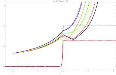
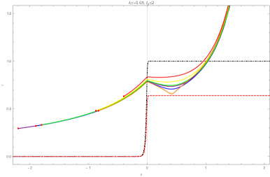
Figure 8: Left panel: $r$ vs $v$ profile of representative geodesics with $\lambda_{GB}=-0.05$ and fixed $\ell=1.35$. Right panel: $r$ vs $v$ profile of representative geodesics with $\lambda_{GB}=-0.05$ and fixed $t_{b}=2$

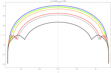
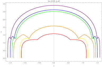
Figure 9: Left panel:$x$ vs $z$ profile of representative geodesics with $\lambda_{GB}=-0.05$ and fixed $\ell=1.35$. Right panel: $x$ vs $z$ profile of representative geodesics with $\lambda=-0.05$ and fixed $t_{b}=2$

References

- (1) S. Ryu and T. Takayanagi, Holographic derivation of entanglement entropy from AdS/CFT, Phys.Rev.Lett. 96 (2006) 181602, [hep-th/0603001].
- (2) J. Abajo-Arrastia, J. Aparicio, and E. Lopez, Holographic Evolution of Entanglement Entropy, JHEP 11 (2010) 149, [arXiv:1006.4090].
- (3) V. E. Hubeny, H. Maxfield, M. Rangamani, and E. Tonni, Holographic entanglement plateaux, JHEP 1308 (2013) 092, [arXiv:1306.4004].
- (4) V. E. Hubeny and H. Maxfield, Holographic probes of collapsing black holes, JHEP 1403 (2014) 097, [arXiv:1312.6887].
- (5) H. Liu and S. J. Suh, Entanglement growth during thermalization in holographic systems, Phys.Rev. D89 (2014), no. 6 066012, [arXiv:1311.1200].
- (6) B. Freivogel, R. A. Jefferson, L. Kabir, B. Mosk, and I.-S. Yang, Casting Shadows on Holographic Reconstruction, arXiv:1412.5175.
- (7) V. E. Hubeny and M. Rangamani, Causal Holographic Information, JHEP 1206 (2012) 114, [arXiv:1204.1698].
- (8) V. Balasubramanian, B. D. Chowdhury, B. Czech, and J. de Boer, Entwinement and the emergence of spacetime, JHEP 1501 (2015) 048, [arXiv:1406.5859].
- (9) A. Buchel, J. Escobedo, R. C. Myers, M. F. Paulos, A. Sinha, et al., Holographic GB gravity in arbitrary dimensions, JHEP 1003 (2010) 111, [arXiv:0911.4257].
- (10) D. M. Hofman and J. Maldacena, Conformal collider physics: Energy and charge correlations, JHEP 0805 (2008) 012, [arXiv:0803.1467].
- (11) X. O. Camanho, J. D. Edelstein, J. Maldacena, and A. Zhiboedov, Causality Constraints on Corrections to the Graviton Three-Point Coupling, arXiv:1407.5597.
- (12) Y.-Z. Li, S.-F. Wu, and G.-H. Yang, Gauss-Bonnet correction to Holographic thermalization: two-point functions, circular Wilson loops and entanglement entropy, Phys.Rev. D88 (2013) 086006, [arXiv:1309.3764].
- (13) X. Zeng and W. Liu, Holographic thermalization in Gauss-Bonnet gravity, Phys.Lett. B726 (2013) 481–487, [arXiv:1305.4841].
- (14) X.-X. Zeng, X.-M. Liu, and W.-B. Liu, Holographic thermalization with a chemical potential in Gauss-Bonnet gravity, JHEP 1403 (2014) 031, [arXiv:1311.0718].
- (15) V. Jahnke, A. S. Misobuchi, and D. Trancanelli, Holographic renormalization and anisotropic black branes in higher curvature gravity, JHEP 01 (2015) 122, [arXiv:1411.5964].
- (16) V. E. Hubeny, M. Rangamani, and T. Takayanagi, A Covariant holographic entanglement entropy proposal, JHEP 0707 (2007) 062, [arXiv:0705.0016].
- (17) V. Balasubramanian, A. Bernamonti, J. de Boer, N. Copland, B. Craps, et al., Holographic Thermalization, Phys.Rev. D84 (2011) 026010, [arXiv:1103.2683].
- (18) E. Caceres and A. Kundu, Holographic Thermalization with Chemical Potential, JHEP 1209 (2012) 055, [arXiv:1205.2354].
- (19) D. Galante and M. Schvellinger, Thermalization with a chemical potential from AdS spaces, JHEP 1207 (2012) 096, [arXiv:1205.1548].
- (20) E. Caceres, A. Kundu, and D.-L. Yang, Jet Quenching and Holographic Thermalization with a Chemical Potential, JHEP 1403 (2014) 073, [arXiv:1212.5728].
- (21) L.-Y. Hung, R. C. Myers, and M. Smolkin, On Holographic Entanglement Entropy and Higher Curvature Gravity, JHEP 1104 (2011) 025, [arXiv:1101.5813].
- (22) J. de Boer, M. Kulaxizi, and A. Parnachev, Holographic Entanglement Entropy in Lovelock Gravities, JHEP 1107 (2011) 109, [arXiv:1101.5781].
- (23) X. Dong, Holographic Entanglement Entropy for General Higher Derivative Gravity, JHEP 1401 (2014) 044, [arXiv:1310.5713].
- (24) J. Camps, Generalized entropy and higher derivative Gravity, JHEP 1403 (2014) 070, [arXiv:1310.6659].
- (25) M. Headrick, V. E. Hubeny, A. Lawrence, and M. Rangamani, Causality and holographic entanglement entropy, JHEP 1412 (2014) 162, [arXiv:1408.6300].
- (26) J. Erdmenger, M. Flory, and C. Sleight, Conditions on holographic entangling surfaces in higher curvature gravity, JHEP 06 (2014) 104, [arXiv:1401.5075].
- (27) X. O. Camanho and J. D. Edelstein, A Lovelock black hole bestiary, Class. Quant. Grav. 30 (2013) 035009, [arXiv:1103.3669].
- (28) R. C. Myers and A. Singh, Comments on Holographic Entanglement Entropy and RG Flows, JHEP 1204 (2012) 122, [arXiv:1202.2068].
- (29) D. G. Boulware and S. Deser, String Generated Gravity Models, Phys. Rev. Lett. 55 (1985) 2656.
- (30) R. C. Myers and B. Robinson, Black Holes in Quasi-topological Gravity, JHEP 08 (2010) 067, [arXiv:1003.5357].
- (31) R.-G. Cai, Gauss-Bonnet black holes in AdS spaces, Phys. Rev. D65 (2002) 084014, [hep-th/0109133].
- (32) R. Callan, J.-Y. He, and M. Headrick, Strong subadditivity and the covariant holographic entanglement entropy formula, JHEP 06 (2012) 081, [arXiv:1204.2309].
- (33) E. Caceres, A. Kundu, J. F. Pedraza, and W. Tangarife, Strong Subadditivity, Null Energy Condition and Charged Black Holes, JHEP 1401 (2014) 084, [arXiv:1304.3398].
- (34) P. Figueras, V. E. Hubeny, M. Rangamani, and S. F. Ross, Dynamical black holes and expanding plasmas, JHEP 0904 (2009) 137, [arXiv:0902.4696].
- (35) J. Dormand and P. Prince, A family of embedded runge-kutta formulae, Journal of Computational and Applied Mathematics 6 (1980), no. 1 19 – 26.
- (36) E. Hairer, G. Wanner, DoP853, 1994.
- (37) A. Allais and E. Tonni, Holographic evolution of the mutual information, JHEP 01 (2012) 102, [arXiv:1110.1607].
- (38) P. Fonda, L. Franti, V. Ker nen, E. Keski-Vakkuri, L. Thorlacius, and E. Tonni, Holographic thermalization with Lifshitz scaling and hyperscaling violation, JHEP 08 (2014) 051, [arXiv:1401.6088].
- (39) M. Alishahiha, A. F. Astaneh, and M. R. M. Mozaffar, Thermalization in backgrounds with hyperscaling violating factor, Phys. Rev. D90 (2014), no. 4 046004, [arXiv:1401.2807].
- (40) P. Bueno and P. F. Ramirez, Higher-curvature corrections to holographic entanglement entropy in geometries with hyperscaling violation, JHEP 12 (2014) 078, [arXiv:1408.6380].
- (41) G. Knodel and J. T. Liu, Higher derivative corrections to Lifshitz backgrounds, JHEP 10 (2013) 002, [arXiv:1305.3279].
- (42) S. Bhattacharyya and S. Minwalla, Weak Field Black Hole Formation in Asymptotically AdS Spacetimes, JHEP 09 (2009) 034, [arXiv:0904.0464].
- (43) E. Caceres, A. Kundu, J. F. Pedraza, and D.-L. Yang, Weak Field Collapse in AdS: Introducing a Charge Density, arXiv:1411.1744.