Probabilistic Programming with Gaussian Process Memoization

Abstract

Gaussian Processes (GPs) are widely used tools in statistics, machine learning, robotics, computer vision, and scientific computation. However, despite their popularity, they can be difficult to apply; all but the simplest classification or regression applications require specification and inference over complex covariance functions that do not admit simple analytical posteriors. This paper shows how to embed Gaussian processes in any higher-order probabilistic programming language, using an idiom based on memoization, and demonstrates its utility by implementing and extending classic and state-of-the-art GP applications. The interface to Gaussian processes, called gpmem, takes an arbitrary real-valued computational process as input and returns a statistical emulator that automatically improve as the original process is invoked and its input-output behavior is recorded. The flexibility of gpmem is illustrated via three applications: (i) Robust GP regression with hierarchical hyper-parameter learning, (ii) discovering symbolic expressions from time-series data by fully Bayesian structure learning over kernels generated by a stochastic grammar, and (iii) a bandit formulation of Bayesian optimization with automatic inference and action selection. All applications share a single 50-line Python library and require fewer than 20 lines of probabilistic code each.

Keywords: Probabilistic Programming, Gaussian Processes, Structure Learning, Bayesian Optimization

1 Introduction

Gaussian Processes (GPs) are widely used tools in statistics (Barry, 1986), machine learning (Neal, 1995; Williams and Barber, 1998; Kuss and Rasmussen, 2005; Rasmussen and Williams, 2006; Damianou and Lawrence, 2013), robotics (Ferris et al., 2006), computer vision (Kemmler et al., 2013), and scientific computation (Kennedy and O’Hagan, 2001; Schneider et al., 2008; Kwan et al., 2013). They are also central to probabilistic numerics, an emerging effort to develop more computationally efficient numerical procedures, and to Bayesian optimization, a family of meta-optimization techniques that are widely used to tune parameters for deep learning algorithms (Snoek et al., 2012; Gelbart et al., 2014). They have even seen use in artificial intelligence. For example, by searching over structured kernels generated by a stochastic grammar, the “Automated Statistician” system can produce symbolic descriptions of time series  (Duvenaud et al., 2013) that can be translated into natural language (Lloyd et al., 2014).

This paper shows how to integrate GPs into higher-order probabilistic programming languages and illustrates the utility of this integration by implementing it for the Venture platform. The key idea is to use GPs to implement a kind of “statistical” or “generalizing” memoization. The resulting higher-order procedure, called gpmem, takes a kernel function and a source function and returns a GP-based statistical emulator for the source function that can be queried at locations where the source function has not yet been evaluated. When the source function is invoked, new datapoints are incorporated into the emulator. In principle, the covariance function for the GP is also allowed to be an arbitrary probabilistic program. This simple packaging covers the full range of uses of the GP described above, including both statistical applications and applications to scientific computation and uncertainty quantification.

This paper illustrates gpmem by embedding it in Venture, a general-purpose, higher-order probabilistic programming platform (Mansinghka et al., 2014). Venture has several distinctive capabilities that are needed for the applications in this paper. First, it supports a flexible foreign interface for modeling components that supports the efficient rank-1 updates required by standard GP implementations. Second, it provides inference programming constructs that can be used to describe custom inference strategies that combine elements of gradient-based, Monte Carlo, and variational inference techniques. This level of control over inference is key to state-of-the-art applications of GPs. Third, it supports models with stochastic recursion, a priori unbounded support sets, and higher-order procedures; together, these enable the combination of stochastic grammars with a fast GP implementation, needed for structure learning. Fourth, Venture permits nesting of modeling and inference, which is needed for the use of GPs in Bayesian optimization over general objective functions that may in general themselves be derived from modeling and inference.

To the best of our knowledge, this is the first general-purpose integration of GPs into a probabilistic programming language. Unlike software libraries such as GPy (The GPy authors, 2012–2015), our embedding allows uses of GPs that go beyond classification and regression to include state-of-the art applications in structure learning and meta-optimization.

This paper presents three applications of gpmem: (i) a replication of results by Neal (1997) on outlier rejection via hyper-parameter inference; (ii) a fully Bayesian extension to the Automated Statistician project; and (iii) an implementation of Bayesian optimization via Thompson sampling. The first application can in principle be replicated in several other probabilistic languages embedding the proposal that is described in this paper. The remaining two applications rely on distinctive capabilities of Venture: support for fully Bayesian structure learning and language constructs for inference programming. All applications share a single 50-line Python library and require fewer than 20 lines of probabilistic code each.

2 Background on Gaussian Processes

Gaussian Processes (GPs) are a Bayesian method for regression. We consider the regression input to be real-valued scalars $x_{i}$ and the regression output $f(x_{i})=y_{i}$ as the value of a function $f$ at $x_{i}$. The complete training data will be denoted by column vectors $\mathbf{x}$ and $\mathbf{y}$. Unseen test input is denoted with $\mathbf{x}^{\prime}$. Gaussian Processes (GP)s present a non-parametric way to express prior knowledge on the space of all possible functions $f$ modeling a regression relationship. Formally, a GP is an infinite-dimensional extension of the multivariate Gaussian distribution.

The collection of random variables $\left\{f(x_{i})=y_{i}\right\}$ (indexed by $i$) represents the values of the function $f$ at each location $x_{i}$. We write $f\sim\mathcal{GP}(\mu,k\mid\bm{\theta}_{\text{mean}},\bm{\theta})$, where $\mu$ is the mean function and $k$ is the covariance function or kernel. That is, $\mu(x_{i}\mid\bm{\theta}_{\text{mean}})$ is the prior mean of the random variable $y_{i}$, and $k(x_{i},x_{j}\mid\bm{\theta})$ is the prior covariance of the random variables $y_{i}$ and $y_{j}$. The output of both mean and covariance function are conditioned on a few free hyper-parameters parameterizing $k$ and $\mu$. We refer to these hyper-parameters as $\bm{\theta}$ and $\bm{\theta}_{\text{mean}}$ respectively. To simplify the calculation below, we will assume the prior mean $\mu$ is identically zero; once the derivation is done, this assumption can be easily relaxed via translation. We use upper case italic $K(\mathbf{x},\mathbf{x}^{\prime}\mid\bm{\theta})$ for a function that returns a matrix of dimension $I\times J$ with entries $k(x_{i},x_{j}\mid\bm{\theta})$ and with $x_{i}\in\mathbf{x}$ and $x_{j}\in\mathbf{x}^{\prime}$ where $I$ and $J$ indicate the length of the column vectors $\mathbf{x}$ and $\mathbf{x}^{\prime}$. Throughout, we write $\mathbf{K}_{(\bm{\theta},\mathbf{x},\mathbf{x}^{\prime})}$ for the prior covariance matrix that results from computing $K(\mathbf{x},\mathbf{x}^{\prime}\mid\bm{\theta})$. In the following, we will sometimes drop the subscript $\mathbf{x},\mathbf{x}^{\prime}$, writing only $\mathbf{K}_{\bm{\theta}}$, for clarity. Note that we do this only in cases when both input vectors are identical and correspond to training input $\mathbf{x}$. We differentiate two different situations leading to different ways samples can be generated with this setup:

1. ${\mathbf{y}^{\prime}}$ - the predictive posterior sample from a distribution conditioned on observed input $\mathbf{x}$ with observed output $\mathbf{y}$ and conditioned on $\bm{\theta}$.

2. $\mathbf{y}^{*}$ - a sample from the predictive prior. We will describe situations, where the GP has not seen any data $\mathbf{x},\mathbf{y}$ yet. In this case, we sample from a Gaussian distribution with $\mathbf{y}^{*}\sim\mathcal{N}\big{(}0,K(\mathbf{x}^{*},\mathbf{x}^{*}\mid\bm{\theta})\big{)}$; where the symbol $*$ indicates that no data has been observed yet.

We now show how to compute the predictive posterior distribution of test output $\mathbf{y}^{\prime}:=f(\mathbf{x}^{\prime})$ conditioned on training data $\mathbf{y}:=f(\mathbf{x})$. (Here $\mathbf{x}$ and $\mathbf{x}^{\prime}$ are known constant vectors, and we are conditioning on an observed value of $\mathbf{y}$.) The predictive posterior can be computed by first forming the joint density when both training and test data are treated as randomly chosen from the prior, then fixing the value of $\mathbf{y}$ to a constant. To start, let

$$\Sigma:=\begin{bmatrix}K(\mathbf{x},\mathbf{x}\mid\bm{\theta})&K(\mathbf{x},\mathbf{x}^{\prime}\mid\bm{\theta})\\ K(\mathbf{x}^{\prime},\mathbf{x}\mid\bm{\theta})&K(\mathbf{x}^{\prime},\mathbf{x}^{\prime}\mid\bm{\theta})\end{bmatrix}\text{ and }\Sigma^{-1}=:\begin{bmatrix}\mathbf{M}_{11}&\mathbf{M}_{12}\\ \mathbf{M}_{21}&\mathbf{M}_{22}\end{bmatrix}.$$

We then have

$$P(\mathbf{y},\mathbf{y}^{\prime}\mid\bm{\theta})\propto\exp\left\{-\frac{1}{2}\begin{bmatrix}\mathbf{y}^{\top}&\mathbf{y}^{\prime\top}\end{bmatrix}\begin{bmatrix}\mathbf{M}_{11}&\mathbf{M}_{12}\\ \mathbf{M}_{21}&\mathbf{M}_{22}\end{bmatrix}\begin{bmatrix}\mathbf{y}\\ \mathbf{y}^{\prime}\end{bmatrix}\right\}.$$

Treating $\mathbf{y}$ as a fixed constant, we obtain

$$P\left(\mathbf{y}^{\prime}\ \middle|\ \mathbf{y},\bm{\theta}\right)\propto P(\mathbf{y},\mathbf{y}^{\prime}\mid\bm{\theta})\propto\exp\left\{-\frac{1}{2}\mathbf{y}^{\prime\top}\mathbf{M}_{22}\mathbf{y}^{\prime}-\mathbf{h}^{\top}\mathbf{y}^{\prime}\right\},$$

where $\mathbf{h}=M_{21}\mathbf{y}$ is a constant vector. Thus $P(\mathbf{y}^{\prime}|\mathbf{y},\bm{\theta})$ is Gaussian,

$$P\left(\mathbf{y}^{\prime}\ \middle|\ \mathbf{y},\bm{\theta}\right)\sim\mathcal{N}(\bm{\mu}_{\bm{\theta}}^{\text{post}},\mathbf{K}_{\bm{\theta}}^{\text{post}}),$$ (1)

with covariance matrix $\mathbf{K}_{\bm{\theta}}^{\text{post}}=\mathbf{M}_{22}^{-1}$. To find its mean $\bm{\mu}_{\bm{\theta}}^{\text{post}}$, we note that $P_{\mathbf{y}^{\prime}|\mathbf{y},\bm{\theta}}(\mathbf{y}^{\prime}+\bm{\mu}_{\bm{\theta}}^{\text{post}})$ is Gaussian with the same covariance as $P(\mathbf{y}^{\prime}|\mathbf{y},\bm{\theta})$, but its exponent has no linear term:

$$P_{\mathbf{y}^{\prime}|\mathbf{y},\bm{\theta}}\left(\mathbf{y}^{\prime}+\bm{\mu}_{\bm{\theta}}^{\text{post}}\ \middle|\ \mathbf{y},\bm{\theta}\right) \propto\exp\left\{-\frac{1}{2}(\mathbf{y}^{\prime}+\bm{\mu}_{\bm{\theta}}^{\text{post}})^{\top}\mathbf{M}_{22}(\mathbf{y}^{\prime}+\bm{\mu}_{\bm{\theta}}^{\text{post}})-\mathbf{h}^{\top}(\mathbf{y}^{\prime}+\bm{\mu}_{\bm{\theta}}^{\text{post}})\right\}$$

$$\propto\exp\left\{-\frac{1}{2}\mathbf{y}^{\prime}\top\mathbf{M}_{22}\mathbf{y}^{\prime}-\underbrace{(\mathbf{h}+\mathbf{M}_{22}\bm{\mu}_{\bm{\theta}}^{\text{post}})^{\top}}_{\text{must be $0$}}\mathbf{y}^{\prime}\right\}.$$

Thus $\mathbf{h}=-\mathbf{M}_{22}\bm{\mu}_{\bm{\theta}}^{\text{post}}$ and $\bm{\mu}_{\bm{\theta}}^{\text{post}}=-\mathbf{M}_{22}^{-1}\mathbf{h}=-\mathbf{M}_{22}^{-1}\mathbf{M}_{21}\mathbf{y}$.

The partioned inverse equations (Barnett and Barnett, 1979 following MacKay, 1998) give

$$\mathbf{M}_{22} =\big{(}K(\mathbf{x}^{\prime},\mathbf{x}^{\prime}\mid\bm{\theta})-K(\mathbf{x}^{\prime},\mathbf{x}\mid\bm{\theta})K(\mathbf{x},\mathbf{x}\mid\bm{\theta})^{-1}K(\mathbf{x},\mathbf{x}^{\prime}\mid\bm{\theta})\big{)}^{-1},$$

$$\mathbf{M}_{21} =-\mathbf{M}_{22}K(\mathbf{x}^{\prime},\mathbf{x}\mid\bm{\theta})K(\mathbf{x},\mathbf{x}\mid\bm{\theta})^{-1}.$$

Substituting these in the above gives

$$\mathbf{K}_{\bm{\theta}}^{\text{post}} =K(\mathbf{x}^{\prime},\mathbf{x}^{\prime}\mid\bm{\theta})-K(\mathbf{x}^{\prime},\mathbf{x}\mid\bm{\theta})K(\mathbf{x},\mathbf{x}\mid\bm{\theta})^{-1}K(\mathbf{x},\mathbf{x}^{\prime}\mid\bm{\theta}),$$ (2)

$$\bm{\mu}_{\bm{\theta}}^{\text{post}} =K(\mathbf{x}^{\prime},\mathbf{x}\mid\bm{\theta})K(\mathbf{x},\mathbf{x}\mid\bm{\theta})^{-1}\mathbf{y}.$$ (3)

Together, $\bm{\mu}_{\bm{\theta}}^{\text{post}}$ and $\mathbf{K}_{\bm{\theta}}^{\text{post}}$ determine the computation of the predictive posterior with unseen input data (1).

Often one assumes the observed regression output is noisily measured, that is, one only sees the values of $\mathbf{y}_{\textrm{noisy}}=\mathbf{y}+\mathbf{w}$ where $\mathbf{w}$ is Gaussian white noise with variance $\sigma_{\textrm{noise}}^{2}$. This noise term can be absorbed into the covariance function $K(\mathbf{x},\mathbf{x}\mid\bm{\theta})$. The log-likelihood of a GP can then be written as:

$$\log P(\mathbf{y}\mid\mathbf{x},\bm{\theta})=-\frac{1}{2}\mathbf{y}^{\top}\mathbf{K}_{\bm{\theta}}^{-1}\mathbf{y}-\frac{1}{2}\log\left\lvert\mathbf{K}_{\bm{\theta}}\right\rvert-\frac{n}{2}\log 2\pi$$ (4)

where $n$ is the number of data points. Both log-likelihood and predictive posterior can be computed efficiently using a Stochastic Process (SP) in Venture (Mansinghka et al., 2014) with an algorithm that resorts to Cholesky factorization(Rasmussen and Williams, 2006, chap. 2). We write the Cholesky factorization as $\mathbf{L}\coloneqq\text{chol}(\mathbf{K}_{\bm{\theta}})$ when :

$$\mathbf{K}_{\bm{\theta}}=\mathbf{L}\mathbf{L}^{\top}$$ (5)

where $\mathbf{L}$ is a lower triangular matrix. This allows us to compute the inverse of a covariance matrix as

$$\mathbf{K}_{\bm{\theta}}^{-1}=(\mathbf{L}^{-1})^{\top}(\mathbf{L}^{-1})$$ (6)

and its determinant as

$$det(\mathbf{K}_{\bm{\theta}})=det(\mathbf{L})^{2}$$ (7)

We compute (4) as

$$\log(P(\mathbf{y}\mid\mathbf{x},\bm{\theta})\coloneqq-\frac{1}{2}\mathbf{y}^{\top}\bm{\alpha}-\sum_{i}\log\mathbf{L}_{ii}-\frac{n}{2}\log 2\pi$$ (8)

where

$$\mathbf{L}\coloneqq\text{chol}(\mathbf{K}_{\bm{\theta}})$$ (9)

and

$$\bm{\alpha}\coloneqq\mathbf{L}^{\top}\backslash(\mathbf{L}\backslash\mathbf{y}).$$ (10)

This results in a computational complexity for sampling in the number of data points of $O(n^{3}/6)$ for (9) an $O(n^{2}/2)$ for (10). Above, we defined the GP prior as $\mathbf{y}^{*}\sim\mathcal{N}\big{(}0,K(\mathbf{x}_{*},\mathbf{x}_{*}\mid\bm{\theta})\big{)}$. We see that this prior is fully determined by its covariance function.

2.1 Covariance Functions

The covariance function (or kernel) of a GP governs high-level properties of the observed data such as smoothness or linearity. The high-level properties are indicated with superscript on functions. A linear covariance can be written as:

$$k^{\text{linear}}=\sigma_{1}^{2}(xx^{\prime}).$$ (11)

We can also express periodicity:

$$k^{\text{periodic}}=\sigma_{2}^{2}\exp\bigg{(}\frac{2\sin^{2}(\pi(x-x^{\prime})/p}{\ell^{2}}\bigg{)}.$$ (12)

By changing these properties we get completely different prior behavior for sampling $\mathbf{y}^{*}$ from a GP with a linear kernel

$$\mathbf{y}^{*}\sim\mathcal{N}\big{(}0,K^{\text{linear}}(\mathbf{x}^{*},\mathbf{x}^{*}\mid\sigma_{1})\big{)}$$

as compared to sampling from the prior predictive with a periodic kernel (as depicted in Fig. 1 (c) and (d))

$$\mathbf{y}^{*}\sim\mathcal{N}\big{(}0,K^{\text{periodic}}(\mathbf{x}^{*},\mathbf{x}^{*}\mid\sigma_{2},\ell)\big{)}.$$

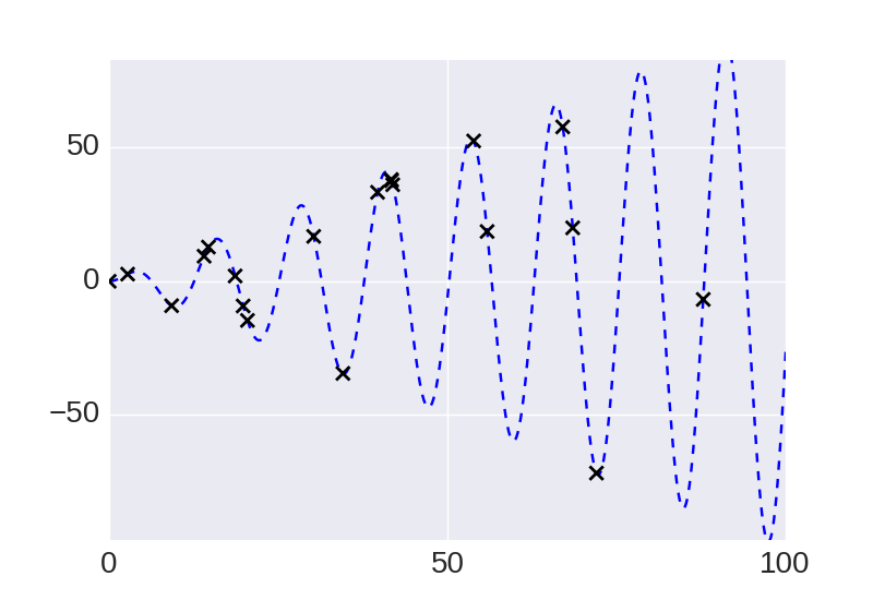
(a) Raw Data

$$k^{\text{linear}} =\sigma_{1}^{2}(xx^{\prime})$$

$$k^{\text{periodic}} =\sigma_{2}^{2}\exp\bigg{(}\frac{2\sin^{2}(\pi(x-x^{\prime})/p}{\ell^{2}}\bigg{)}$$

$$k^{\text{linear}}\times k^{\text{periodic}} =\sigma_{1}^{2}(xx^{\prime})\,\sigma_{2}^{2}\exp\bigg{(}\frac{2\sin^{2}(\pi(x-x^{\prime})/p}{\ell^{2}}\bigg{)}$$

(b) Kernels

Prior predictive, $\mathbf{y}^{*}\sim\mathcal{N}\big{(}0,K(\mathbf{x}^{*},\mathbf{x}^{*}\mid\bm{\theta})\big{)}$:

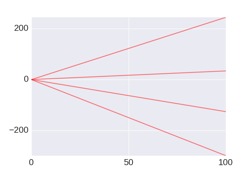
(c) $K^{\text{linear}}$

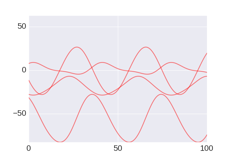
(d) $K^{\text{periodic}}$

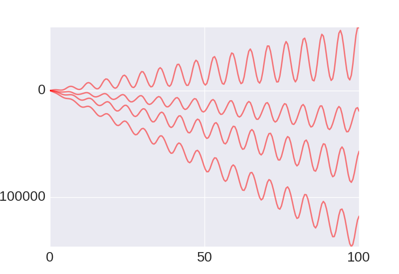
(e) $K^{\text{linear}}\times K^{\text{periodic}}$

Posterior predictive $\mathbf{y}^{\prime}\sim\mathcal{N}(\bm{\mu}_{\bm{\theta}}^{\text{post}},\mathbf{K}_{\bm{\theta}}^{\text{post}})$:

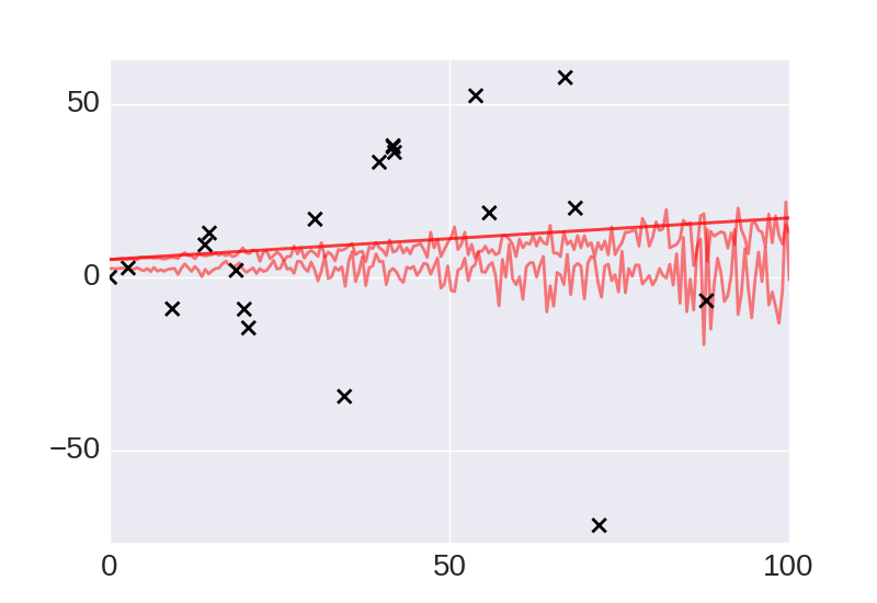
(f) $K^{\text{linear}}$

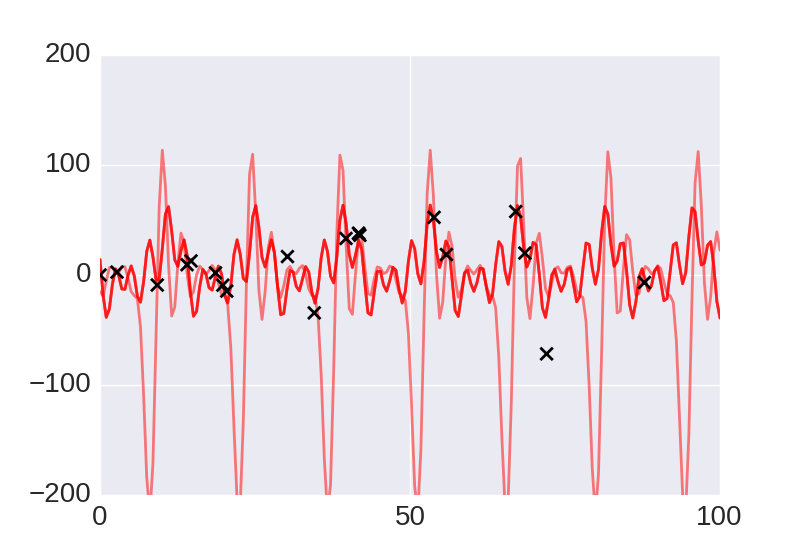
(g) $K^{\text{periodic}}$

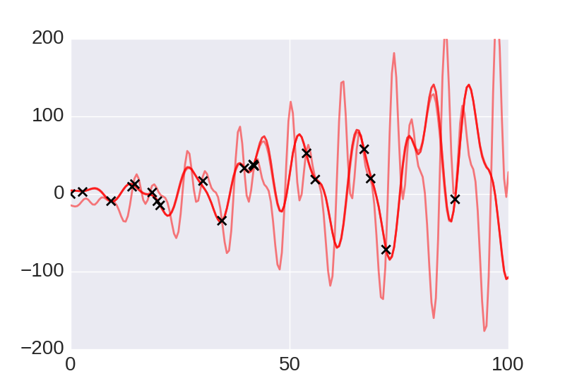
(h) $K^{\text{linear}}\times K^{\text{periodic}}$

Figure 0: We depict kernel composition. (a) shows raw data (black) generated with a sine function with linearly growing amplitude (blue). This data is used for all the plots (c-h). (b) shows the linear and the periodic base kernel in functional form as well as a composition of both. The multiplication of the two kernels indicates local interaction. The local interaction we account for in this case is the growing amplitude (a). For each column (c-h) $\bm{\theta}$ is different.(c-e) show samples from the prior predictive $\mathbf{y}^{*}$ where random parameters are used, that is, we sample before any data points are observed. (f-h) show samples from the predictive posterior $\mathbf{y}^{\prime}$, after the data has been observed.

These high-level properties are compositional via addition and multiplication of different covariance functions. That means that we can also combine these properties. By using multiplication of kernels we can model a local interaction of two components, for example

$$k^{\text{linear}}\times k^{\text{periodic}}=\sigma_{1}^{2}(xx^{\prime})\,\sigma_{2}^{2}\exp\bigg{(}\frac{2\sin^{2}(\pi(x-x^{\prime})/p}{\ell^{2}}\bigg{)}.$$ (13)

This results in a combination of the higher level properties of linearity and periodicity. In Fig 1 (e) we depict samples for $\mathbf{y}^{*}$ that are periodic with linearly increasing amplitude. We consider this a local interaction because the actual interaction depends on the similarity of two data points. An addition of covariance functions models a global interaction, that is an interaction of two high-level components that is qualitatively not dependent on the input space. An example for this a periodic function with a linear trend.

For each kernel type, each $\bm{\theta}$ is different, that is, in (11) we have $\bm{\theta}=\{\sigma_{1}\}$, in (12) we have $\bm{\theta}=\{\sigma_{2},p,\ell\}$ and in (13) we have $\bm{\theta}=\{\sigma_{1},\sigma_{2},p,\ell\}$. Adjusting these hyper-parameters changes lower level qualitative attributes such as length scales ($\ell$) while preserving the higher level qualitative properties of the distribution such as linearity.

If we choose a suitable set of hyper-parameters, for example by performing inference, we can capture the underlying dynamics of the data well (see Fig. 1 (f-h)) while sampling $\mathbf{y}^{\prime}$. Note that goodness of fit is not only limited to the parameters. A too simple qualitative structure implies unsuitable behaviour, as for example in (Fig. 1 (g)) where additional recurring spikes are introduced to account for the changing amplitude of the true function that generated the data.

3 Gaussian Process Memoization in Venture

Memoization is the practice of storing previously computed values of a function so that future calls with the same inputs can be evaluated by lookup rather than re-computation. To transfer this idea to probabilistic programming, we now introduce a language construct called a statistical memoizer. Suppose we have a function f which can be evaluated but we wish to learn about the behavior of f using as few evaluations as possible. The statistical memoizer, which here we give the name gpmem, was motivated by this purpose. It produces two outputs:

$$\texttt{f}\xrightarrow{\texttt{gpmem}}(\texttt{f}_{\text{compute}},\texttt{f}_{\textrm{emu}}).$$

The function $\texttt{f}_{compute}$ calls f and stores the output in a memo table, just as traditional memoization does. The function $\texttt{f}_{\textrm{emu}}$ is an online statistical emulator which uses the memo table as its training data. A fully Bayesian emulator, modelling the true function f as a random function $f\sim P(f)$, would satisfy

$$\texttt{(}\texttt{f}_{\textrm{emu}}\ \texttt{x}_{1}\ \ldots\ \texttt{x}_{k}\texttt{)}\sim P\left(f(\texttt{x}_{1}),\ldots,f(\texttt{x}_{k})\ \middle|\ \text{$f(\texttt{x})=\texttt{(f x)}$ for each $\texttt{x}$ in memo table}\right).$$

Different implementations of the statistical memoizer can have different prior distributions $P(f)$; in this paper, we deploy a GP prior (implemented as gpmem below). Note that we require the ability to sample $\texttt{f}_{\textrm{emu}}$ jointly at multiple inputs because the values of $f(\texttt{x}_{1}),\ldots,f(\texttt{x}_{k})$ will in general be dependent.

⬇

define f = proc(x) {exp(-0.1*abs(x-2)) * 10 * cos(0.4*x) + 0.2};Ωassume sf = tag(scope="hyper-parameters", gamma(5,1));Ωassume l = tag(scope="hyper-parameters", gamma(5,1));Ωassume kse = apply_function(make_squaredexp(sf, l));

⬇

assume (f_compute, f_emu) = gpmem(f, kse);Ωsample f_emu(array(-20, $\cdots$, 20));

⬇

predict f_compute(12.6);Ωsample f_emu(array(-20, $\cdots$, 20));

⬇

predict f_compute(-6.4);Ωsample f_emu(array(-20, $\cdots$, 20));

⬇

observe f_emu(-3.1) = 2.60;Ωobserve f_emu(7.8) = -7.60;Ωobserve f_emu(0.0) = 10.19;Ωsample f_emu(array(-20, $\cdots$, 20));

⬇

infer mh(scope="hyper-parameter", steps=50);Ωsample f_emu(array(-20, $\cdots$, 20));

(b)(c)(d)(e)(f)(g)

Figure 1: gpmem tutorial. The top shows a schematic of gpmem. f_compute probes an outside resource. This can be expensive (top left). Every probe is memoized and improves the emulator. Below the schematic we see the evolution of gpmem’s state of believe of the world given certain Venture directives. On the right, we depict the true function (blue), samples from the emulator (red) and incorporated observations (black).

We explain how gpmem, the statistical memoizer with GP-prior, works using a simple tutorial (Fig. 1). The top panel (Fig. 1, (a)) of this figure sketches the schematic of gpmem. f is the external process that we memoize. It can be evaluated using resources that potentially come from outside of Venture. We feed this function into gpmem alongside a parameterised kernel $k$. In this example, we make the qualitative assumption of $f$ being smooth, and define $k$ to be a squared-exponential covariance function:

$$k=k^{\text{se}}=\sigma^{2}\exp(-\frac{(x-x^{\prime})^{2}}{2\ell^{2}}).$$

The hyper-parameters $\bm{\theta}$ for this kernel are sampled from a prior distribution which is depicted in the top right box. Note that we annotate $\bm{\theta}=\{\texttt{sf},\texttt{l}\}$ for subsequent inference as belonging to the scope “hyper-parameter”.

gpmem implements a memoization table, where all previously computed function evaluations ($\{\mathbf{x},\mathbf{y}\}$) are stored. We also initialize a GP-prior that will serve as our statistical emulator:

$$P(f_{emu}(x)\mid\mathbf{x},\mathbf{y},\bm{\theta})\sim\mathcal{N}\big{(}\bm{\mu}_{\bm{\theta}}^{\text{post}},\mathbf{K}_{\bm{\theta}}^{\text{post}})\big{)}$$

where

$$P(f_{emu}(x)\mid\mathbf{x},\mathbf{y},\bm{\theta})=\mathbf{y}^{\prime}$$

under the traditional GP perspective. All value pairs stored in the memoization table ($\text{memo table}=(\mathbf{x},\mathbf{y})$) are incorporated as observations of the GP. We simply feed the regression input into the emulator and output a predictive posterior Gaussian distribution determined by the GP and the memoization table.

We can either define the function f that serves as as input for gpmem natively in Venture (as shown in the Fig. 1 (b)) or we interleave Venture with foreign code. This can be useful when f is computed with the help of outside resources. We define and parameterize a squared-exponential kernel (b) which we then supply to gpmem (Fig. 1 (c)). Before making any observations or calls to f we can sample from the prior at the inputs from -20 to 20 using the emulator :

⬇

assume (f_compute, f_emu) = gpmem(f, kse));ΩΩ sample f_emu(array(-20, ..., 20));

where the second line corresponds to:

$$\mathbf{y}^{*}\sim\mathcal{N}\Bigg{(}0,K^{\text{se}}\bigg{(}\begin{bmatrix}-20\\ \cdots\\ 20\end{bmatrix},\begin{bmatrix}-20\\ \cdots\\ 20\end{bmatrix}\mid\bm{\theta}=\{\sigma,\ell\}\bigg{)}\Bigg{)}.$$

In Fig. 1 (d), we probe the external function f at point 12.6 and memoize its result by calling

⬇

predict f_compute (12.6);

When we subsequently sample from the emulator, that is compute the $\mathbf{y}^{\prime}$ at the input $\mathbf{x}^{\prime}=\begin{bmatrix}-20,\cdots,20\end{bmatrix}^{\top}$, we see how the posterior shifts from uncertainty to near certainty close to the input 12.6.

We can repeat the process at a different point (probing point -6.4 in Fig. 1 (e)) to see that we gain certainty about another part of the curve.

We can add information to $\texttt{f}_{\text{emu}}$ about presumable value pairs of f without calling $\texttt{f}_{\text{compute}}$ (Fig. 1 (f)). If a friend tells us the value of f we can call observe to store this information in the incorporated observations for $\texttt{f}_{\text{emu}}$ only:

⬇

observe f_emu( -3.1) = 2.60;

We have this value pair now available for the computation $\mathbf{y}^{\prime}$. For sampling with the emulator, the effect is the same as calling predict with the $\texttt{f}_{\text{compute}}$. However, we can imagine at least one scenario where such as distinction in the treatment of observations is beneficial. Let us say we do not only have the real function available but also a domain expert with knowledge about this function. This expert could tell us what the value is at a given input. Potentially, the value provided by the expert could disagree with the value computed with f for example due to different levels of observation noise.

Finally, we can update our posterior by inferring the posterior over hyper-parameter values $\bm{\theta}$. For this we use the defined scopes, which tag a collection of related random choices, such as all hyper-parameters $\bm{\theta}$. These tags are supplied to the inference program (in this case, MH) to specify on which random variables inference should be done:

⬇

infer mh(scope="hyper-parameters", steps=50);

In this case, we perform one Metropolis-Hastings (MH) transition over the scope hyper-parameters and choose a random member of this scope, that is we choose one hyper-parameter at random. We can also define custom inference actions. Let’s define MH with Gaussian drift proposals.

⬇

define drift_kernel = proc(x) { normal(x, 1) };ΩΩ define my_markov_chain =Ω apply_mh_correction(Ω subproblem=choose_by_scope("hyper-parameters"),Ω proposal=symmetric_local_proposal_from_chain(drift_kernel))ΩΩ infer my_markov_chain;

Note that this inference is not in the Figure. The important part of the above code snippet is drift_kernel, which is where we say that at each step of our Markov chain, we would like to propose a transition by sampling a new state from a unit normal distribution whose mean is the current state.

The newly inferred hyper-parameters allow us now to adequately reflect uncertainty about the curve given all incorporated observations (compare Fig. 1, bottom panel (g) on the right with the samples before inference, one panel above (f)).

4 Applications

This paper illustrates the flexibility of gpmem by showing how it can concisely encode three different applications of GPs. The first is a standard example from hierarchical Bayesian statistics, where Bayesian inference over a hierarchical hyper-prior is used to provide a curve-fitting methodology that is robust to outliers. The second is a structure learning application from probabilistic artificial intelligence, where GPs are used to discover qualitative structure in time series data. The third is a reinforcement learning application, where GPs are used as part of a Thompson sampling formulation of Bayesian optimization for general real-valued objective functions with real inputs.

4.1 Nonlinear regression in the presence of outliers

We can apply gpmem for regression in a hierarchical Bayesian setting (Fig. 2).

⬇

// Define data and look-up functionΩdefine data = array(array(-1.87, 0.13), ..., array(1.67, 0.81));Ωassume f_look_up = proc(index) {lookup(data, index)};

⬇

// Initialize hyper-priorsΩassume alpha_sf = tag(scope="hyperhyper", gamma(5,1));Ωassume beta_sf = tag(scope="hyperhyper", gamma(5,1));Ωassume alpha_l = tag(scope="hyperhyper", gamma(5,1));Ωassume beta_l = tag(scope="hyperhyper", gamma(5,1));Ωassume sf = tag(scope="hyper", gamma(alpha_sf, beta_sf)));Ωassume l = tag(scope="hyper", gamma(alpha_l, beta_l)));

⬇

// Initialize covariance functionΩassume se = apply_function(make_squaredexp(sf, l));Ωassume wn = apply_function(make_whitenoise(sigma));Ωassume composite_covariance = add_funcs(se, wn);Ω// Create a prober and emulator using gpmemΩassume (f_compute, f_emu) =Ω gpmem(f_look_up, composite_covariance);Ωsample f_emu(array(-2, $\cdots$, 2));

⬇

// Observe all data pointsΩfor (n = 0; n < size(data); n++){Ω observe f_emu(first(lookup(data,n))) =Ω second(lookup(data,n))};Ω// Or: probe all data pointsΩfor (n = 0; n < size(data); n++){Ω predict f_compute(first(lookup(data,n)))};Ωsample f_emu(array(-2, $\cdots$, 2));

⬇

// Metropolis-HastingsΩinfer repeat(100, do(Ω mh(scope="hyperhyper", steps=2),Ω mh(scope="hyper", steps=1)));Ωsample f_emu(array(-2, $\cdots$, 2));

⬇

// OptimizationΩinfer gradient-ascent(scope="hyper",Ω steps=10);ΩΩsample f_emu(array(-2, $\cdots$, 2));

(b)(c)(d)(e)(f)(g)(h)

Figure 2: Regression with outliers and hierarchical prior structure.

In a Bayesian treatment of hyper-parameter learning for GPs, we can write the posterior probability of the hyper-parameters of a GP (Fig. 2, (a)) given covariance function $\bm{\mathcal{K}}=k$ as:

$$P(\bm{\theta}=\{sf,\ell,\sigma\}\mid\mathbf{D},\bm{\mathcal{K}})=\frac{P(\mathbf{D}\mid\bm{\theta},\bm{\mathcal{K}})P(\bm{\theta}\mid\bm{\mathcal{K}})}{P(\mathbf{D}\mid\bm{\mathcal{K}})}$$ (14)

where $\mathbf{D}=\{\mathbf{x},\mathbf{y}\}$ is a training data set and $\bm{\mathcal{K}}$ is treated as a random variable over covariance functions. Since we can apply gpmem to any process or procedure, it can be used in situations where a data set is available only via a look-up function f_look_up. In fact, we demonstrate gpmem’s application to regression using an example where the data was generated by a function which is not available, that is, we do not provide the synthetic function to gpmem but only a data set (Fig. 2 (b)). This function, $f_{\text{true}}$, is taken from a paper on the treatment of outliers with hierarchical Bayesian hyper-priors for GPs (Neal, 1997):

$$f_{\text{true}}(x)=0.3+0.4x+0.5\sin(2.7x)+\frac{1.1}{(1+x^{2})}+\eta\;\;\;with\;\;\eta\sim\mathcal{N}(0,\sigma_{\text{noise}}).$$ (15)

We synthetically generate outliers by setting $\sigma_{\text{noise}}=0.1$ in $95\%$ of the cases and to $\sigma_{\text{noise}}=1$ in the remaining cases. Instead of accessing the $f_{\text{true}}$ directly, we are accessing the data in form of a a two dimensional array with f_look_up.

We set $\bm{\mathcal{K}}=k^{\text{se}+\text{wn}}$ and parameterize it with $\bm{\theta}=\{sf,\ell,\sigma\}$. For these hyper-parameters, Neals work suggests a hierarchical system for hyper-parameterization. Here, we draw hyper-parameters from $\Gamma$ distributions:

$$\ell\sim\Gamma(\alpha_{1},\beta_{1}),\;\sigma\sim\Gamma(\alpha_{2},\beta_{2})$$ (16)

and in turn sample the $\alpha$ and $\beta$ from $\Gamma$ distributions as well:

$$\alpha_{1}\sim\Gamma(\alpha^{1}_{\alpha},\beta^{1}_{\alpha}),\;\alpha_{2}\sim\Gamma(\alpha^{2}_{\alpha},\beta^{2}_{\alpha}),\cdots$$ (17)

We model this in Venture as illustrated in Fig. 2 (c), using the build-in SP gamma.

In Fig. 2, panel (d), we see that $k^{\text{se}+\text{wn}}$ is defined as a composite covariance function. It is the sum (add_funcs) of a squared exponential kernel (make_squaredexp) and a white noise ($k^{\text{wn}}$, Appendix A) kernel which is implemented with make_whitenoise. We then initialize gpmem feeding it with composite_covariance and the data look-up function f_look_up. We sample from the prior $\mathbf{y}^{*}$ with random parameters sf,l and sigma and without any observations available (Fig. 2, panel (e)). We depict those samples on the right (red), alongside the true function that generated the data (blue) and the data points we have available in the data set (black).

We can incorporate observations using both observe and predict (Fig. 2 (f)). When we subsequently sample $\mathbf{y}^{\prime}$ from the emulator with $\mathcal{N}(\bm{\mu}_{\bm{\theta}}^{\text{post}},\mathbf{K}_{\bm{\theta}}^{\text{post}})$, we can see that the GP posterior incorporates knowledge about the data. Yet, the hyper-parameters sf,l and sigma are still random, so the emulator does not capture the true underlying dynamics ($f_{\text{true}}$) of the data correctly.

Next, we demonstrate how we can capture these underlying dynamics within only 100 nested MH steps on the hyper-parameters to get a good approximation for their posterior $\mathbf{y}^{\prime}$ (Fig. 2 (g)). We say nested because we first take two sweeps in the scope hyperhyper which characterizes (17) and then one sweep on the scope hyper which characterizes (16). This is repeated 100 times using $\texttt{repeat( 100, do(}\cdots\;$. Note that Neal devises an additional noise model and performs a large number of Hybrid-Monte Carlo and Gibbs steps to achieve this, whereas inference in Venture with gpmem is merely one line of code.

Finally, we can change our inference strategy altogether. If we decide that instead of following a Bayesian sampling approach, we would like to perform empirical optimization, we do this by only changing one line of code, deploying gradient-ascent instead of mh (Fig. 2 (h)).

4.2 Discovering qualitative structure from time series data

Inductive learning of symbolic expressions for continuous-valued time series data is a hard task which has recently been tackled using a greedy search over the approximate posterior of the possible kernel compositions for GPs (Duvenaud et al., 2013; Lloyd et al., 2014).

With gpmem we can provide a fully Bayesian treatment of this, previously unavaible, using a stochastic grammar (see Fig. 3).

(a)

(d)

Base Kernels (BK)
LIN: Linearity	PER: Periodicity	SE: Smoothness	WN: White Noise

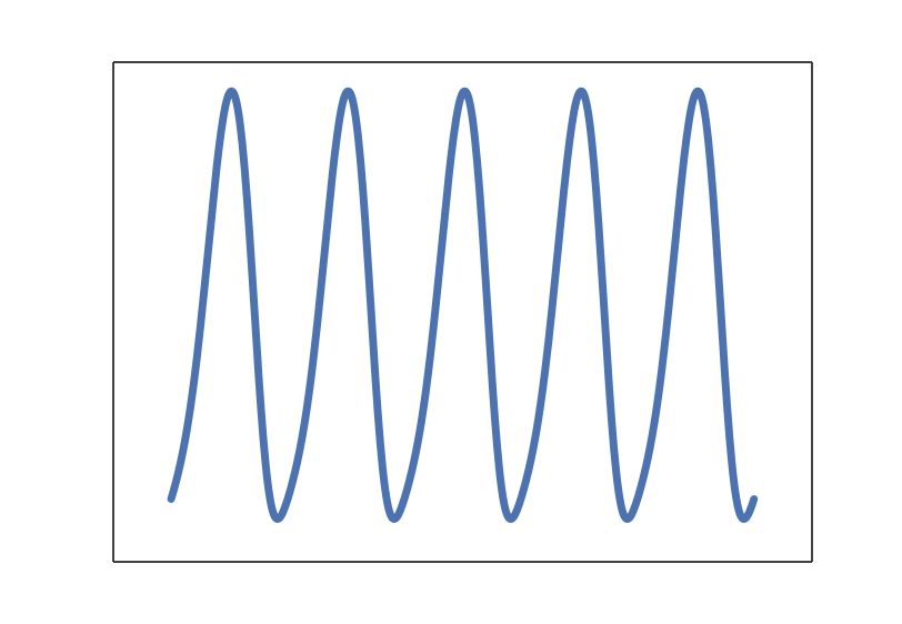
Composite Structure
LIN + PER:	LIN $\times$ PER:	SE $\times$ PER:	LIN $\times$ LIN:
Periodicity with Trend	Growing Amplitude	Local Periodicity	Quadratic

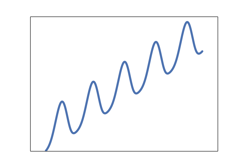
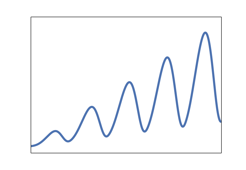
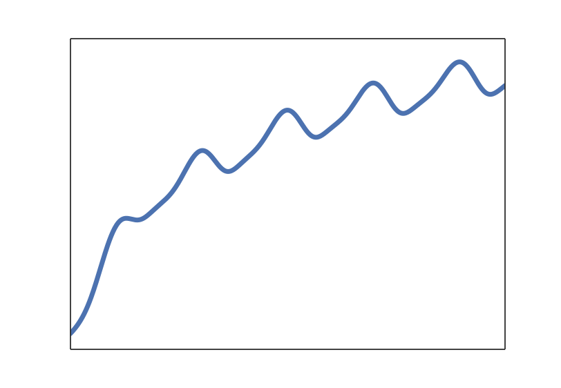
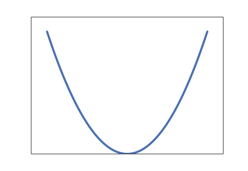
(e)

Figure 3: (a) Bayesian GP structure learning. A set of base kernels (BK) with priors on their hyper-parameters serves as hypothesis space and is supplied as input to the stochastic grammar. The stochastic grammar has two parts: (i) a sampler that selects a random set $\mathbf{S}$ of primitive kernels from BK and (ii) a kernel composer that combines the individual base kernels and generates a composite kernel function $k_{\bm{\theta}}$. This serves as input for gpmem. We observe value pairs $\mathbf{x},\mathbf{y}$ of unstructured time series data on the bottom of the schematic. (b) We use $\text{Parse}(k_{\bm{\theta}})$ to parse a structure. (c) kernel functions are simplified with the $\text{Simplify}()$-operator. The simplifed $k_{\bm{\theta}}$ is used as input for $\text{Struct}()$ (d) which interprets it symbolically. Base kernels and compositional kernels are shown in (e) alongside their interpretation with Struct().

This allows us to read an unstructured time series and automatically output a high-level, qualitative description of it. The stochastic grammar takes a set of primitive base kernels $\text{BK}=\{k_{\bm{\theta}^{1}}^{1},\cdots,k_{\bm{\theta}^{m}}^{m}\}$

$\bm{\theta}^{*}=\{\bm{\theta}^{1},\cdots,\bm{\theta}^{m}\}$ (Fig. 3 (a) and (b)) We depict the input for the stochastic grammar in Listing 1.

We sample a random subset $\mathbf{S}$ of the set of supplied base kernels. $\mathbf{S}$ is of size $n\leq m$. We write

$$\mathbf{S}=\{k_{\bm{\theta}^{i}}^{i},\cdots,k_{\bm{\theta}^{n}}^{n}\}\sim P(\mathbf{S}=\{k_{\bm{\theta}^{i}}^{i},\cdots,k_{\bm{\theta}^{n}}^{n}\}\mid\text{BK})$$

with

$$P(\mathbf{S}=\{k_{\bm{\theta}^{i}}^{i},\cdots,k_{\bm{\theta}^{n}}^{n}\}\mid\text{BK})=\frac{n!}{\mid\mathbf{S}=\{k_{\bm{\theta}^{i}}^{i},\cdots,k_{\bm{\theta}^{n}}^{n}\}\mid!}.$$

BK is assumed to be fixed as the most general margin of our hypothesis space. In the following, we will drop it in the notation. The only building block that we are now missing is how to combine the sampled base kernels into a compositional covariance function (see Fig. 3 (b)). For each interaction $i$, we have to infer whether the data supports a local interaction or a global interaction, chosing between one out of two algebraic operators $\bm{\Omega}_{i}=\{+,\times\}$. The probability for all such decisions is given by a binomial distribution:

$$P(\bm{\Omega}\mid\mathbf{S})={n\choose r}p_{+\times}^{r}(1-p_{+\times})^{n-r}.$$ (18)

We can write the marginal probability of a kernel function as

$$P(\bm{\mathcal{K}}\mid\mathbf{x},\mathbf{y},\bm{\theta})=\iint\limits_{\bm{\Omega},\mathbf{S}}P(\bm{\mathcal{K}}\mid\mathbf{x},\mathbf{y},\bm{\theta},\bm{\Omega},\mathbf{S})\times P(\bm{\Omega}\mid\mathbf{S})\times P(\mathbf{S})\;\text{\bf d}\bm{\Omega}\,\text{\bf d}\mathbf{S}\,$$ (19)

with $\bm{\theta}\subseteq\bm{\theta}^{*}$ as implied by $\mathbf{S}$. For structure learning with GP kernels, a composite kernel is sampled from $P(\bm{\mathcal{K}})$ and fed into gpmem. The emulator generated by gpmem observes unstructured time series data. Venture code for the probabilistic grammar is shown in Listing 2, code for inference with gpmem in Listing 3. Listing 1: Initialize Base Kernels BK and $P(n)$ ⬇ innerleftmargininnerlinewidthmiddlelinewidthouterlinewidthlinewidth1   // Initialize hyper-parametersΩinnerleftmargininnerlinewidthmiddlelinewidthouterlinewidthlinewidth2  assume theta_1 = tag(scope="hyper-parameters", gamma(5,1));Ωinnerleftmargininnerlinewidthmiddlelinewidthouterlinewidthlinewidth3  assume theta_2 = tag(scope="hyper-parameters", gamma(5,1));Ωinnerleftmargininnerlinewidthmiddlelinewidthouterlinewidthlinewidth4  assume theta_3 = tag(scope="hyper-parameters", gamma(5,1));Ωinnerleftmargininnerlinewidthmiddlelinewidthouterlinewidthlinewidth5  assume theta_4 = tag(scope="hyper-parameters", gamma(5,1));Ωinnerleftmargininnerlinewidthmiddlelinewidthouterlinewidthlinewidth6  assume theta_5 = tag(scope="hyper-parameters", gamma(5,1));Ωinnerleftmargininnerlinewidthmiddlelinewidthouterlinewidthlinewidth7  assume theta_6 = tag(scope="hyper-parameters", gamma(5,1));Ωinnerleftmargininnerlinewidthmiddlelinewidthouterlinewidthlinewidth8  assume theta_7 = tag(scope="hyper-parameters", gamma(5,1));Ωinnerleftmargininnerlinewidthmiddlelinewidthouterlinewidthlinewidth9  Ωinnerleftmargininnerlinewidthmiddlelinewidthouterlinewidthlinewidth11   // Make kernelsΩinnerleftmargininnerlinewidthmiddlelinewidthouterlinewidthlinewidth12  assume lin = apply_function(make_linear, theta_1);Ωinnerleftmargininnerlinewidthmiddlelinewidthouterlinewidthlinewidth13  assume per = apply_function(make_periodic, theta_2, theta_3, theta_4);Ωinnerleftmargininnerlinewidthmiddlelinewidthouterlinewidthlinewidth14  assume se = apply_function(make_squaredexp, theta_5, theta_6);Ωinnerleftmargininnerlinewidthmiddlelinewidthouterlinewidthlinewidth15  assume wn = apply_function(make_noise, theta_7);Ωinnerleftmargininnerlinewidthmiddlelinewidthouterlinewidthlinewidth16  Ωinnerleftmargininnerlinewidthmiddlelinewidthouterlinewidthlinewidth17  // Initialize the set of primitive base kernels BKΩinnerleftmargininnerlinewidthmiddlelinewidthouterlinewidthlinewidth18  assume BK = list(lin, per, se, wn);

Many equivalent covariance structures can be sampled due to covariance function algebra and equivalent representations with different parameterization (Lloyd et al., 2014). To inspect the posterior of these equivalent structures we convert each kernel expression into a sum of products and subsequently simplify. We introduce three different operators that work on kernel functions:

1. $\text{Parse}(k)$, an operator that parses a covariance function (Fig. 3 (b)).

2. $\text{Simplify}(k)$; this operators simplifies a kernel function $k$ according to the simplifications that we present in Appendix B and Fig. 3 (c).

3. $\text{Struct}(k)$; interprets the structure of a covariance function (Fig. 3 (d) and Appendix C), for example $\text{Struct}(k^{\text{linear}})=\text{LIN}$; it translates the functional structure into a symbolic expression.

All base kernels relevant for this work can be found in Appendix A. Listing 2: Stochastic Grammar ⬇ innerleftmargininnerlinewidthmiddlelinewidthouterlinewidthlinewidth1  // Select a random subset of a set of possible primitive kernels (BK)Ωinnerleftmargininnerlinewidthmiddlelinewidthouterlinewidthlinewidth2  assume select_primitive_kernels = proc(l) {Ωinnerleftmargininnerlinewidthmiddlelinewidthouterlinewidthlinewidth3   if is_null(l) {Ωinnerleftmargininnerlinewidthmiddlelinewidthouterlinewidthlinewidth4   lΩinnerleftmargininnerlinewidthmiddlelinewidthouterlinewidthlinewidth5   } else {Ωinnerleftmargininnerlinewidthmiddlelinewidthouterlinewidthlinewidth6   if bernoulli() {Ωinnerleftmargininnerlinewidthmiddlelinewidthouterlinewidthlinewidth7   pair(first(l), select_primitive_kernels(rest(l)))Ωinnerleftmargininnerlinewidthmiddlelinewidthouterlinewidthlinewidth8   } else {Ωinnerleftmargininnerlinewidthmiddlelinewidthouterlinewidthlinewidth9   select_primitive_kernels(rest(l))Ωinnerleftmargininnerlinewidthmiddlelinewidthouterlinewidthlinewidth10   }Ωinnerleftmargininnerlinewidthmiddlelinewidthouterlinewidthlinewidth11   }Ωinnerleftmargininnerlinewidthmiddlelinewidthouterlinewidthlinewidth12  };Ωinnerleftmargininnerlinewidthmiddlelinewidthouterlinewidthlinewidth13  // Construct the kernel composition with a composer procedureΩinnerleftmargininnerlinewidthmiddlelinewidthouterlinewidthlinewidth14  assume kernel_composer = proc(l) {Ωinnerleftmargininnerlinewidthmiddlelinewidthouterlinewidthlinewidth15   if (size(l) <= 1) {Ωinnerleftmargininnerlinewidthmiddlelinewidthouterlinewidthlinewidth16   first(l)Ωinnerleftmargininnerlinewidthmiddlelinewidthouterlinewidthlinewidth17   } else {Ωinnerleftmargininnerlinewidthmiddlelinewidthouterlinewidthlinewidth18   if (bernoulli()) {Ωinnerleftmargininnerlinewidthmiddlelinewidthouterlinewidthlinewidth19   add_funcs(first(l), kernel_composer(rest(l)))Ωinnerleftmargininnerlinewidthmiddlelinewidthouterlinewidthlinewidth20   } else {Ωinnerleftmargininnerlinewidthmiddlelinewidthouterlinewidthlinewidth21   mult_funcs(first(l), kernel_composer(rest(l)))Ωinnerleftmargininnerlinewidthmiddlelinewidthouterlinewidthlinewidth22   }Ωinnerleftmargininnerlinewidthmiddlelinewidthouterlinewidthlinewidth23   }Ωinnerleftmargininnerlinewidthmiddlelinewidthouterlinewidthlinewidth24  };Ωinnerleftmargininnerlinewidthmiddlelinewidthouterlinewidthlinewidth25  // Select the set primitive kernels that will form the structureΩinnerleftmargininnerlinewidthmiddlelinewidthouterlinewidthlinewidth26  assume primitive_kernel_selection = tag(scope="grammar",Ωinnerleftmargininnerlinewidthmiddlelinewidthouterlinewidthlinewidth27   permute(select_primitive_kernels(BK)));Ωinnerleftmargininnerlinewidthmiddlelinewidthouterlinewidthlinewidth28  // Compose the structureΩinnerleftmargininnerlinewidthmiddlelinewidthouterlinewidthlinewidth29  assume K = tag(scope="grammar",Ωinnerleftmargininnerlinewidthmiddlelinewidthouterlinewidthlinewidth30   kernel_composer(primitive_kernel_selection)); Listing 3: gpmem inference for structure learning: ⬇ innerleftmargininnerlinewidthmiddlelinewidthouterlinewidthlinewidth1  // Apply gpmemΩinnerleftmargininnerlinewidthmiddlelinewidthouterlinewidthlinewidth2  assume (f_compute, f_emu) = gpmem(f_look_up, K);Ωinnerleftmargininnerlinewidthmiddlelinewidthouterlinewidthlinewidth3  // Probe all data pointsΩinnerleftmargininnerlinewidthmiddlelinewidthouterlinewidthlinewidth4  for (n = 0; n < size(data); n++) {Ωinnerleftmargininnerlinewidthmiddlelinewidthouterlinewidthlinewidth5   predict f_compute(first(lookup(data, n)))};Ωinnerleftmargininnerlinewidthmiddlelinewidthouterlinewidthlinewidth6  // Perform inferenceΩinnerleftmargininnerlinewidthmiddlelinewidthouterlinewidthlinewidth7  infer repeat(200, do(Ωinnerleftmargininnerlinewidthmiddlelinewidthouterlinewidthlinewidth8   mh(scope="grammar", steps=1),Ωinnerleftmargininnerlinewidthmiddlelinewidthouterlinewidthlinewidth9   mh(scope="hyper-parameters", steps=2)));

We defined a simple space of covariance structures in a way that allows us to produce results coherent with work presented in Automatic Statistician (Duvenaud et al., 2013; Lloyd et al., 2014). The results are illustrated with two data sets.

Mauna Loa CO₂ data

Figure 4: Structure Learning. Starting with raw data (a), we fit a GP (b) and compute the posterior distribution on structures (c). We take a sample of the peak of this distribution ($\text{LIN}+\text{PER}+\text{SE}+\text{WN}$) including its parameters and write it in functional form (d). We depict the human readable interpretation (e). We used (d) to plot (b).

We illustrate results in Fig 4. In Fig 4 (a) we depict the raw data. We see mean centered CO₂ measurements of the Mauna Loa Observatory, an atmospheric baseline station on Mauna Loa, on the island of Hawaii. A description of the data set can be found in Rasmussen and Williams, 2006, chapter 5. We use those raw data to compute a posterior on structure, parameters and GP samples. The latter are shown in Fig 4 (b) where we zoom in to show how the posterior captures the error bars adequately. This posterior of the GP is generated with a random sample from the parameters of the peak of the distribution on structure (Fig 4 (c)). We differentiate between a posterior distribution of kernel functions and a posterior distribution of symbolic expressions describing different kernel structures. This allows us to compute the posterior of symbollically equivalent structures, such as $\text{Struct}(k^{\text{linear}}+k^{\text{periodic}})=\text{Struct}(k^{\text{periodic}}+k^{\text{linear}})$. Both structures yield and addition of a linear kernel and a periodic kernel, that is LIN + PER. Therefore, we parse $k$ with $\text{Parse}(k)$, we simplify an expression with $\text{Simplify}(k)$ and then compute $\text{Struct}(k)$. For the Mauna Loa Co₂ data, this distribution peaks at:

$$\text{Struct}(\bm{\mathcal{K}}=k)=\text{LIN}+\text{PER}+\text{SE}+\text{WN}.$$ (20)

We write this kernel equation out in Fig 4 (d). This kernel structure has a natural language interpretation that we spell out in Fig 4 (e), explaining that the posterior peaks at a kernel structure with four additive components. Each of which holds globally, that is there are no higher level, qualitative aspects of the data that vary with the input space. The additive components for this result are as follows:

• a linearly increasing function or trend;

• a periodic function;

• a smooth function; and

• white noise.

Previous work on automated kernel discovery (Duvenaud et al., 2013) illustrated the Mauna Loa data using an RQ kernel. We resort to the white noise kernel instead of RQ (similar to (Lloyd et al., 2014)).

Airline Data

The second data set (Fig. 5) we depict results for is the airline data set describing monthly totals of international airline passengers (Box et al., 1997, according to Duvenaud et al., 2013).

Figure 5: Structure Learning. Starting with raw data (a), we fit a GP (b) and compute the posterior distribution on structures (c). We take a sample of the peak of this distribution ($\text{LIN}+\text{PER}\times\text{SE}+\text{WN}$) including its parameters and write it in functional form (d). We depict the human readable interpretation (e). We used (d) to plot (b).

We illustrate results for this data set in Fig 5. In Fig 5 (a) we depict the raw data. Again, the data is mean centered and we use it to compute a posterior on structure, parameters and GP samples. The latter are shown in Fig 5 (b). This posterior of the GP is generated with a random sample from the parameters of the peak of the distribution on structure (Fig 5 (c)). The posterior over symbolic kernel expressions peaks at:

$$\text{Struct}(\bm{\mathcal{K}}=k)=\text{LIN}+\text{SE}\times\text{PER}+\text{WN}.$$ (21)

We write this Kernel equation out in Fig 5 (d). This kernel structure has a natural language interpretation that we spell out in Fig 5 (e), explaining that the posterior peaks at a kernel structure with three additive components. Additive components hold globally, that is there are no higher level, qualitative aspects of the data that vary with the input space. The additive components are as follows:

• a linearly increasing function or trend;

• an approximate periodic function; and

• white noise.

Both datasets served as illustrations in the Automatic Statistician project.

Querying time series

With our Bayesian approach to structure learning we can gain valuable insights into time series data that were previously unavailable. This is due to our ability to estimate posterior marginal probabilities over the kernel structure. Over this marginal, we define boolean search operations that allow us to query the data for the probability of certain structures to hold true globally.

$$P(\text{Struct}(\bm{\mathcal{K}}=k)\mid\mathbf{x},\mathbf{y},\bm{\theta})= \frac{1}{T}\sum\limits_{t=1}^{T}\text{Contains}(k,k^{t})$$ (22)

$$\text{where}\,\text{Contains}(k,k^{t})=\begin{cases}1,&\text{if }k\underset{global}{\in}k^{t},\\ 0,&\text{otherwise}.\end{cases}$$ (23)

to ask whether it is true that a global structure $\bm{\mathcal{K}}=k$ is present. $T$ is the number of all posterior samples for $\bm{\mathcal{K}}$ and $k^{t}$ is one such sample. $\underset{global}{\in}k^{t}$ reads as “is one of $k^{t}$’s global functional components”. We can now ask simple questions, for example:

Is there white noise in the data?

To answer this question we set $\text{Struct}(\bm{\mathcal{K}})=$WN in (22). We write this in shorthand as $\text{WN}(\bm{\mathcal{K}})$. Similarly, we write $\text{LIN}(\bm{\mathcal{K}})$, $\text{PER}(\bm{\mathcal{K}})$ and $\text{SE}(\bm{\mathcal{K}})$. We can also formulate more sophisticated search operations using Boolean operators such as AND ($\land$) and OR ($\lor$). The AND operator is defined as follows:

$$P(\text{Struct}(\bm{\mathcal{K}}^{a}=k^{a})\,\land\,\text{Struct}(\bm{\mathcal{K}}^{b}=k^{b})\mid\mathbf{x},\mathbf{y},\bm{\theta})=\frac{1}{N}\sum\limits_{n=1}^{N}\text{Contains}(k^{a},k^{t})\,\land\,\text{Contains}(k^{b},k^{t})\;\;$$

where

$$\text{Contains}(k^{a},k^{t})\land\text{Contains}(k^{b},k^{t})=\begin{cases}1,&\text{if }k^{a}\,\text{and}\,k^{b}\underset{global}{\in}k^{t},\\ 0,&\text{otherwise}\end{cases}.$$

Figure 6: Querying structural motifs in in time series using posterior inference over kernel structure. The kernel structure serves as a way to formulate natural language questions about the data (blue). The initial question of interest (top) is a fairly general one: “What is the probability of a trend, a recurring pattern and noise in the data?” Below the natural language version of this question, the same question is formulated as an inference problem (black) over the marginal probability on kernels with Boolean operators AND ($\land$) and OR ($\lor$). To gain a deeper understanding of specific motifs in the time series more specific queries can be written. On the right, a query asks whether there is noise in the data (blue) by computing the disjunction of the marginal of a global white noise kernel and a multiplication between a linear and a white noise kernel (black). Samples from the predictive prior $\mathbf{y}_{*}$ of such kernels give an indication of the qualitative aspects that a kernel structure implies (coloured curves below the marginal). If the probability that there is noise in the data is high, it makes sense to drill even deeper asking more detailed questions. With regards to noise, this translates to querying whether or not the data supports the hypothesis that there is heteroskedastic noise or white noise. Queries for motifs of repeating structure are shown in the middle of the tree, queries related to trends on the left.

By estimating $P(\text{LIN}(\bm{\mathcal{K}})\land\text{WN}(\bm{\mathcal{K}})\mid\mathbf{x},\mathbf{y},\bm{\theta})$ we can use this operator to ask questions such as

Is there a linear component AND a white noise in the data?

Finally, we define the logical OR as

$$P(\text{Struct}(\bm{\mathcal{K}}^{a})\,\lor\,\text{Struct}(\bm{\mathcal{K}}^{b})\mid\mathbf{x},\mathbf{y},\bm{\theta})= P(\text{Struct}(\bm{\mathcal{K}}^{a})\mid\mathbf{x},\mathbf{y},\bm{\theta})+P(\text{Struct}(\bm{\mathcal{K}}^{b})\mid\mathbf{x},\mathbf{y},\bm{\theta})$$

$$-P(\text{Struct}(\bm{\mathcal{K}}^{a})\land\text{Struct}(\bm{\mathcal{K}}^{b})\mid\mathbf{x},\mathbf{y},\bm{\theta})$$

where we drop $=k$ for readability. This allows us to ask questions about structures that are logically connected with OR, such as:

Is there white noise or heteroskedastic noise?

by estimating $P(\text{LIN}(\bm{\mathcal{K}})\times\text{WN}(\bm{\mathcal{K}})\;\;{\large\lor}\;\;\text{WN}(\bm{\mathcal{K}})\mid\mathbf{x},\mathbf{y},\bm{\theta})$. We know that noise can either be heteroskedastic or white, and we also know due to simple manipulations using kernel algebra that $\text{LIN}\times\text{WN}$ and WN are the only possible ways to construct noise with kernel composition. This allows us to generalize the question above to:

Is there noise in the data?

where we write the marginal posterior on qualitative structure for noise:

$$P\big{(}\text{Struct}(\bm{\mathcal{K}})=\text{Noise}\mid\mathbf{x},\mathbf{y},\bm{\theta}\big{)}=P(\text{LIN}(\bm{\mathcal{K}})\times\text{WN}(\bm{\mathcal{K}})\;\;{\large\lor}\;\;\text{WN}(\bm{\mathcal{K}})\mid\mathbf{x},\mathbf{y},\bm{\theta}).$$ (24)

From a methodological perspective, this allows us to start with general queries and subsequently formulate follow up queries that go into more detail. For example, we could start with a general query, such as:

What is the probability of a trend, a recurring pattern and noise in the data?

and then follow up with more detailed questions (Fig 6).

This way of querying data for their statistical implications is in stark contrast to what previous research in automatic kernel construction was able to provide. We could view our approach as a time series search engine which allows us to test whether or not certain structures can be found in an available time series. Another way to view this approach is as a new language to interact with the world. Real-world observations often come with time-stamps and in form of continuous valued sensor measurements. We provide the toolbox to query such observations in a similar manner as one would query a knowledge base in a logic programming language.

4.3 Bayesian optimization

The final application demonstrating the power of gpmem illustrates its use in Bayesian optimization. We introduce Thompson sampling, the basic solution strategy underlying the Bayesian optimization with gpmem. Thompson sampling Thompson (1933) is a widely used Bayesian framework for addressing the trade-off between exploration and exploitation in multi-armed (or continuum-armed) bandit problems. We cast the multi-armed bandit problem as a one-state Markov decision process (MDP), and describe how Thompson sampling can be used to choose actions for that MDP.

The MDP can be described as follows: An agent is to take a sequence of actions $x_{1},x_{2},\ldots$ from a (possibly infinite) set of possible actions $\mathcal{X}$. After each action, a reward $y\in\mathbb{R}$ is received, according to an unknown conditional distribution $P_{\textrm{true}}\left(y\ \middle|\ x\right)$. The agent’s goal is to maximize the total reward received for all actions in an online manner. In Thompson sampling, the agent accomplishes this by placing a prior distribution $P(\vartheta)$ on the possible “contexts” $\vartheta\in\Theta$. Here a context is a believed model of the conditional distributions $\{P\left(x\ \middle|\ y\right)\}_{x\in\mathcal{X}}$, or at least, a believed statistic of these conditional distributions which is sufficient for deciding an action $x$. If actions are chosen so as to maximize expected reward, then one such sufficient statistic is the believed conditional mean $V\left(x\ \middle|\ \vartheta\right)=\mathbb{E}\left[y\ \middle|\ x;\vartheta\right]$, which can be viewed as a believed value function. For consistency with what follows, we will assume our context $\vartheta$ takes the form $(\bm{\theta},\mathbf{x},\mathbf{y})$ where $\mathbf{x}$ is the vector of past actions, $\mathbf{y}$ is the vector of their rewards, and $\bm{\theta}$ (the “semicontext”) contains any other information that is included in the context.

In this setup, Thompson sampling has the following steps:

Repeat as long as desired:

1. Sample. Sample a semicontext $\bm{\theta}\sim P(\bm{\theta})$.

2. Search (and act). Choose an action $x\in\mathcal{X}$ which (approximately) maximizes $V\left(x\ \middle|\ \vartheta\right)=\mathbb{E}\left[y\ \middle|\ x;\vartheta\right]=\mathbb{E}\left[y\ \middle|\ x;\,\bm{\theta},\mathbf{x},\mathbf{y}\right]$.

3. Update. Let $y_{\textrm{true}}$ be the reward received for action $x$. Update the believed distribution on $\bm{\theta}$, i.e., $P(\bm{\theta})\leftarrow P_{\textrm{new}}(\bm{\theta})$ where $P_{\textrm{new}}(\bm{\theta})=P\left(\bm{\theta}\ \middle|\ x\mapsto y_{\textrm{true}}\right)$.

Algorithm 1 Thompson sampling.

Note that when $\mathbb{E}\left[y|x;\vartheta\right]$ (under the sampled value of $\bm{\theta}$ for some points $x$) is far from the true value $\mathbb{E}_{P_{\textrm{true}}}\left[y\ \middle|\ x\right]$, the chosen action $x$ may be far from optimal, but the information gained by probing action $x$ will improve the belief $\vartheta$. This amounts to “exploration.” When $\mathbb{E}\left[y\ \middle|\ x;\vartheta\right]$ is close to the true value except at points $x$ for which $\mathbb{E}\left[y\ \middle|\ x;\vartheta\right]$ is low, exploration will be less likely to occur, but the chosen actions $x$ will tend to receive high rewards. This amounts to “exploitation.” The trade-off between exploration and exploitation is illustrated in Figure 7. Roughly speaking, exploration will happen until the context $\vartheta$ is reasonably sure that the unexplored actions are probably not optimal, at which time the Thompson sampler will exploit by choosing actions in regions it knows to have high value.

\begin{overpic}[width=455.3023pt]{figs/slide2.pdf} \put(150.0,300.0){{\parbox{173.44534pt}{\tiny\@@amsalign E\left(x^{\prime}\ \middle|\ x\right)&=-\frac{1}{s}\left(\widetilde{\mu}(x^{\prime})-\widetilde{\mu}(x)\right)\\ \widetilde{\mu}(x)&=\frac{1}{N_{\textrm{avg}}}\sum_{i=1}^{N_{\textrm{avg}}}\widetilde{y}_{i,x}\\ \widetilde{y}_{i,x}=\mathbf{y}^{\prime}&\sim\mathcal{N}(\bm{\mu}_{\bm{\theta}}^{\text{post}},\mathbf{K}_{\bm{\theta}}^{\text{post}}\mid\sigma,\ell,\mathbf{x},\mathbf{y})\\ Q_{\textrm{proposal}}\left(x^{\prime}\ \middle|\ x\right)&\sim\mathcal{N}(x,\,\texttt{propstd}^{2})}}} \put(118.0,331.0){$\tau_{\textrm{search}}$:} \put(62.0,58.0){{\parbox{173.44534pt}{\tiny\@@amsalign P(\sigma,\ell\mid\mathbf{x},\mathbf{y})&\propto\exp\big{\{}{-\frac{1}{2}}\mathbf{y}^{\top}K^{\text{se}}(\mathbf{x},\mathbf{x})^{-1}\mathbf{y}\big{\}}\\ Q_{\textrm{proposal}}\left(\sigma^{\prime},\ell\ \middle|\ \sigma,\ell\right)&=P(\sigma^{\prime})\\ Q_{\textrm{proposal}}\left(\sigma,\ell^{\prime}\ \middle|\ \sigma,\ell\right)&=P(\ell^{\prime})\\ P_{\textrm{accept}}\left(\sigma^{\prime},\ell^{\prime}\ \middle|\ \sigma,\ell,\mathbf{x},\mathbf{y}\right)&=\frac{P\left(\sigma\right)P\left(\ell\right)}{P\left(\sigma^{\prime}\right)P\left(\ell^{\prime}\right)}\exp\bigg{\{}{-\frac{1}{2}}\big{(}\mathbf{y}^{\top}\mathbf{K}_{\bm{\theta}}\left(\mathbf{x},\mathbf{x}\ \middle|\ \sigma^{\prime},\ell^{\prime}\right)^{{-1}}\mathbf{y}-\\ &\;\;\;\;\;\;\;\;\;\;\;\;\;\;\;\;\;\;\;\;\;\;\;\;\;\;\;\;\;\;\;\;\;\;\;\mathbf{y}^{\top}\mathbf{K}_{\bm{\theta}}\left(\mathbf{x},\mathbf{x}\ \middle|\ \sigma,\ell\right)^{{-1}}\mathbf{y}\big{)}\bigg{\}}\\ k^{\text{se}}(\mathbf{x},\mathbf{x})&=\bigg{[}\sigma^{2}\exp\big{\{}{-\frac{(x_{1}-x_{2})^{2}}{2\ell}}\big{\}}\bigg{]}_{x_{1},x_{2}\in\mathbf{x}}}}} \put(65.0,112.0){$\tau_{\textrm{update}}$:} \put(252.0,78.0){\bigg{\}} \footnotesize MH} \put(250.0,102.0){ \} \footnotesize True posterior } \end{overpic}

Figure 7: Two possible actions (in green) for an iteration of Thompson sampling. The believed distribution on the value function $V$ is depicted in red. In this example, the true reward function is deterministic, and is drawn in blue. The action on the right receives a high reward, while the action on the left receives a low reward but greatly improves the accuracy of the believed distribution on $V$. The transition operators $\tau_{\textrm{search}}$ and $\tau_{\textrm{update}}$ are described in Section 4.3.

Typically, when Thompson sampling is implemented, the search over contexts $\vartheta\in\Theta$ is limited by the choice of representation. In traditional programming environments, $\bm{\theta}$ often consists of a few numerical parameters for a family of distributions of a fixed functional form. With work, a mixture of a few functional forms is possible; but without probabilistic programming machinery, implementing a rich context space $\Theta$ would be an unworkably large technical burden. In a probabilistic programing language, however, the representation of heterogeneously structured or infinite-dimensional context spaces is quite natural. Any computable model of the conditional distributions $\left\{P\left(y\ \middle|\ x\right)\right\}_{x\in\mathcal{X}}$ can be represented as a stochastic procedure $(\lambda(x)\ldots)$. Thus, for computational Thompson sampling, the most general context space $\widehat{\Theta}$ is the space of program texts. Any other context space $\Theta$ has a natural embedding as a subset of $\widehat{\Theta}$.

A Mathematical Specification

We now describe a particular case of Thompson sampling with the following properties:

• The regression function has a Gaussian process prior.

• The actions $x_{1},x_{2},\ldots\in\mathcal{X}$ are chosen by a Metropolis-like search strategy with Gaussian drift proposals.

• The hyperparameters of the Gaussian process are inferred using Metropolis–Hastings sampling after each action.

In this version of Thompson sampling, the contexts $\vartheta$ are Gaussian processes over the action space $\mathcal{X}=[-20,20]\subseteq\mathbb{R}$. That is,

$$V\sim\mathcal{GP}(\mu,k),$$

where the mean $\mu$ is a computable function $\mathcal{X}\to\mathbb{R}$ and the covariance $k$ is a computable (symmetric, positive-semidefinite) function $\mathcal{X}\times\mathcal{X}\to\mathbb{R}$. This represents a Gaussian process $\left\{R_{a}\right\}_{a\in\mathcal{X}}$, where $R_{x}$ represents the reward for action $x$. We write past actions as $\mathbf{x}$ and past rewards as $\mathbf{y}$. Computationally, we represent a context as a data structure

$$\vartheta=(\bm{\theta},\mathbf{x},\mathbf{y})=(\mu,k,\bm{\theta},\mathbf{x},\mathbf{y}),$$

where $\bm{\mu}$ is a procedure to be used as the prior mean function and $k$ is a procedure to be used as the prior covariance function, parameterized by $\bm{\theta}$. As above set $\mu\equiv 0$.

Note that the context space $\Theta$ is not a finite-dimensional parametric family, since the vectors $\mathbf{x}$ and $\mathbf{y}$ grow as more samples are taken. $\Theta$ is, however, representable as a computational procedure together with parameters and past samples, as we do in the representation $\vartheta=(\mu,k,\bm{\theta},\mathbf{x},\mathbf{y})$.

We combine the Update and Sample steps of Algorithm 1 by running a Metropolis–Hastings (MH) sampler whose stationary distribution is the posterior $P\left(\bm{\theta}\ \middle|\ \mathbf{x},\mathbf{y}\right)$. The functional forms of $\mu$ and $k$ are fixed in our case, so inference is only done over the parameters $\bm{\theta}=\left\{\sigma,\ell\right\}$; hence we equivalently write $P\left(\sigma,\ell\ \middle|\ \mathbf{x},\mathbf{y}\right)$ for the stationary distribution. We make MH proposals to one variable at a time, using the prior as proposal distribution:

$$Q_{\textrm{proposal}}\left(\sigma^{\prime},\ell\ \middle|\ \sigma,\ell\right)=P(\sigma^{\prime})$$

and

$$Q_{\textrm{proposal}}\left(\sigma,\ell^{\prime}\ \middle|\ \sigma,\ell\right)=P(\ell^{\prime}).$$

The MH acceptance probability for such a proposal is

$$P_{\textrm{accept}}\left(\sigma^{\prime},\ell^{\prime}\ \middle|\ \sigma,\ell\right)=\min\left\{1,\ \frac{Q_{\textrm{proposal}}\left(\sigma,\ell\ \middle|\ \sigma^{\prime},\ell^{\prime}\right)}{Q_{\textrm{proposal}}\left(\sigma^{\prime},\ell^{\prime}\ \middle|\ \sigma,\ell\right)}\cdot\frac{P\left(\mathbf{x},\mathbf{y}\ \middle|\ \sigma^{\prime},\ell^{\prime}\right)}{P\left(\mathbf{x},\mathbf{y}\ \middle|\ \sigma,\ell\right)}\right\}$$

Because the priors on $\sigma$ and $\ell$ are uniform in our case, the term involving $Q_{\textrm{proposal}}$ equals $1$ and we have simply

$$P_{\textrm{accept}}\left(\sigma^{\prime},\ell^{\prime}\ \middle|\ \sigma,\ell\right) =\min\left\{1,\ \frac{P\left(\mathbf{x},\mathbf{y}\ \middle|\ \sigma^{\prime},\ell^{\prime}\right)}{P\left(\mathbf{x},\mathbf{y}\ \middle|\ \sigma,\ell\right)}\right\}$$

$$=\min\bigg{\{}1,\ \exp\bigg{(}-\frac{1}{2}\bigg{(}\mathbf{y}^{T}K\left(\mathbf{x},\mathbf{x}\ \middle|\ \sigma^{\prime},\ell^{\prime}\right)^{-1}\mathbf{y}$$

$$\qquad\qquad\qquad\qquad\qquad-\mathbf{y}^{T}K\left(\mathbf{x},\mathbf{x}\ \middle|\ \sigma,\ell\right)^{-1}\mathbf{y}\bigg{)}\bigg{)}\bigg{\}}.$$

The proposal and acceptance/rejection process described above define a transition operator $\tau_{\textrm{update}}$ which is iterated a specified number of times; the resulting state of the MH Markov chain is taken as the sampled semicontext $\bm{\theta}$ in Step 1 of Algorithm 1.

For Step 2 (Search) of Thompson sampling, we explore the action space using an MH-like transition operator $\tau_{\textrm{search}}$. As in MH, each iteration of $\tau_{\textrm{search}}$ produces a proposal which is either accepted or rejected, and the state of this Markov chain after a specified number of steps is the new action $x$. The Markov chain’s initial state is the most recent action, and the proposal distribution is Gaussian drift:

$$Q_{\textrm{proposal}}\left(x^{\prime}\ \middle|\ x\right)\sim\mathcal{N}(x,\,\texttt{propstd}^{2}),$$

where the drift width propstd is specified ahead of time. The acceptance probability of such a proposal is

$$P_{\textrm{accept}}\left(x^{\prime}\ \middle|\ x\right)=\min\left\{1,\ \exp\left(-E\left(x^{\prime}\ \middle|\ x\right)\right)\right\},$$

where the energy function $E\left(\bullet\ \middle|\ a\right)$ is given by a Monte Carlo estimate of the difference in value from the current action:

$$E\left(x^{\prime}\ \middle|\ x\right)=-\frac{1}{s}\left(\widetilde{\mu}(x^{\prime})-\widetilde{\mu}(x)\right)$$

where

$$\widetilde{\mu}(x)=\frac{1}{N_{\textrm{avg}}}\sum_{i=1}^{N_{\textrm{avg}}}\widetilde{y}_{i,x}$$

and

$$\widetilde{y}_{i,x}=\mathbf{y}^{\prime}\sim\mathcal{N}(\bm{\mu}_{\bm{\theta}}^{\text{post}},\mathbf{K}_{\bm{\theta}}^{\text{post}})$$

and $\left\{\widetilde{y}_{i,x}\right\}_{i=1}^{N_{\textrm{avg}}}$ are i.i.d. for a fixed $x$. (In the above, $\bm{\mu}_{\bm{\theta}}^{\text{post}}$ and $\mathbf{K}_{\bm{\theta}}^{\text{post}}$ are the mean and variance of a posterior sample at the single point $\mathbf{x}^{\prime}=(x^{\prime})$.) Here the temperature parameter $s\geq 0$ and the population size $N_{\textrm{avg}}$ are specified ahead of time. Proposals of estimated value higher than that of the current action are always accepted, while proposals of estimated value lower than that of the current action are accepted with a probability that decays exponentially with respect to the difference in value. The rate of the decay is determined by the temperature parameter $s$, where high temperature corresponds to generous acceptance probabilities. For $s=0$, all proposals of lower value are rejected; for $s=\infty$, all proposals are accepted. For points $x$ at which the posterior mean $\bm{\mu}_{\bm{\theta}}^{\text{post}}$ is low but the posterior variance $\mathbf{K}_{\bm{\theta}}^{\text{post}}$ is high, it is possible (especially when $N_{\textrm{avg}}$ is small) to draw a “wild” value of $\widetilde{\mu}(x)$, resulting in a favorable acceptance probability.

Indeed, taking an action $x$ with low estimated value but high uncertainty serves the useful function of improving the accuracy of the estimated value function at points near $x$ (see Figure 7).^, We see a complete probabilistic program with gpmem implementing Bayesian optimization with Thompson Sampling and both, uniform proposals and drift proposals below (Listing 4,5 and 6). Listing 4: Initialize gpmem for Bayesian optimization ⬇ innerleftmargininnerlinewidthmiddlelinewidthouterlinewidthlinewidth1  assume sf = tag(scope="hyper", uniform_continuous(0, 10));Ωinnerleftmargininnerlinewidthmiddlelinewidthouterlinewidthlinewidth2  assume l = tag(scope="hyper", uniform_continuous(0, 10));Ωinnerleftmargininnerlinewidthmiddlelinewidthouterlinewidthlinewidth3  assume se = make_squaredexp(sf, l);Ωinnerleftmargininnerlinewidthmiddlelinewidthouterlinewidthlinewidth4  assume blackbox_f = get_bayesopt_blackbox();Ωinnerleftmargininnerlinewidthmiddlelinewidthouterlinewidthlinewidth5  assume (f_compute, f_emulate) = gpmem(blackbox_f, se); Listing 5: Bayesian optimization with uniformly distributed proposals ⬇ innerleftmargininnerlinewidthmiddlelinewidthouterlinewidthlinewidth1  // A naive estimate of the argmax of the given functionΩinnerleftmargininnerlinewidthmiddlelinewidthouterlinewidthlinewidth2  define mc_argmax = proc(func) {Ωinnerleftmargininnerlinewidthmiddlelinewidthouterlinewidthlinewidth3   candidate_xs = mapv(proc(i) {uniform_continuous(-20, 20)},Ωinnerleftmargininnerlinewidthmiddlelinewidthouterlinewidthlinewidth4   arange(20));Ωinnerleftmargininnerlinewidthmiddlelinewidthouterlinewidthlinewidth5   candidate_ys = mapv(func, candidate_xs);Ωinnerleftmargininnerlinewidthmiddlelinewidthouterlinewidthlinewidth6   lookup(candidate_xs, argmax_of_array(candidate_ys))Ωinnerleftmargininnerlinewidthmiddlelinewidthouterlinewidthlinewidth7  };Ωinnerleftmargininnerlinewidthmiddlelinewidthouterlinewidthlinewidth8  Ωinnerleftmargininnerlinewidthmiddlelinewidthouterlinewidthlinewidth9  // Shortcut to sample the emulator at a single point without packingΩinnerleftmargininnerlinewidthmiddlelinewidthouterlinewidthlinewidth10  // and unpacking arraysΩinnerleftmargininnerlinewidthmiddlelinewidthouterlinewidthlinewidth11  define emulate_pointwise = proc(x) {Ωinnerleftmargininnerlinewidthmiddlelinewidthouterlinewidthlinewidth12   run(sample(lookup(f_emulate(array(unquote(x))), 0)))Ωinnerleftmargininnerlinewidthmiddlelinewidthouterlinewidthlinewidth13  };Ωinnerleftmargininnerlinewidthmiddlelinewidthouterlinewidthlinewidth14  Ωinnerleftmargininnerlinewidthmiddlelinewidthouterlinewidthlinewidth15  // Main inference loopΩinnerleftmargininnerlinewidthmiddlelinewidthouterlinewidthlinewidth16  infer repeat(15, do(pass,Ωinnerleftmargininnerlinewidthmiddlelinewidthouterlinewidthlinewidth17   // Probe V at the point mc_argmax(emulate_pointwise)Ωinnerleftmargininnerlinewidthmiddlelinewidthouterlinewidthlinewidth18   predict(f_compute(unquote(mc_argmax(emulate_pointwise)))),Ωinnerleftmargininnerlinewidthmiddlelinewidthouterlinewidthlinewidth15   // Infer hyper-parametersΩinnerleftmargininnerlinewidthmiddlelinewidthouterlinewidthlinewidth20   mh(scope="hyper", steps=50))); Listing 6: Bayesian optimization with Gaussian drift proposals ⬇ innerleftmargininnerlinewidthmiddlelinewidthouterlinewidthlinewidth1  // A naive estimate of the argmax of the given functionΩinnerleftmargininnerlinewidthmiddlelinewidthouterlinewidthlinewidth2  define mc_argmax = proc(func) {Ωinnerleftmargininnerlinewidthmiddlelinewidthouterlinewidthlinewidth3   candidate_xs = mapv(proc(x) {normal(x, 1)},Ωinnerleftmargininnerlinewidthmiddlelinewidthouterlinewidthlinewidth4   fill(20,last));Ωinnerleftmargininnerlinewidthmiddlelinewidthouterlinewidthlinewidth5   candidate_ys = mapv(func, candidate_xs);Ωinnerleftmargininnerlinewidthmiddlelinewidthouterlinewidthlinewidth6   lookup(candidate_xs, argmax_of_array(candidate_ys))Ωinnerleftmargininnerlinewidthmiddlelinewidthouterlinewidthlinewidth7  };Ωinnerleftmargininnerlinewidthmiddlelinewidthouterlinewidthlinewidth8  Ωinnerleftmargininnerlinewidthmiddlelinewidthouterlinewidthlinewidth9  // Shortcut to sample the emulator at a single point without packingΩinnerleftmargininnerlinewidthmiddlelinewidthouterlinewidthlinewidth10  // and unpacking arraysΩinnerleftmargininnerlinewidthmiddlelinewidthouterlinewidthlinewidth11  define emulate_pointwise = proc(x) {Ωinnerleftmargininnerlinewidthmiddlelinewidthouterlinewidthlinewidth12   run(sample(lookup(f_emulate(array(unquote(x))), 0)))Ωinnerleftmargininnerlinewidthmiddlelinewidthouterlinewidthlinewidth13  };Ωinnerleftmargininnerlinewidthmiddlelinewidthouterlinewidthlinewidth15  Ωinnerleftmargininnerlinewidthmiddlelinewidthouterlinewidthlinewidth16  // Initialize helper variablesΩinnerleftmargininnerlinewidthmiddlelinewidthouterlinewidthlinewidth17  assume previous_point = uniform_continuous(-20,20);Ωinnerleftmargininnerlinewidthmiddlelinewidthouterlinewidthlinewidth18  run(observe(previous_point ,run(sample(previous_point)),prev));Ωinnerleftmargininnerlinewidthmiddlelinewidthouterlinewidthlinewidth19  Ωinnerleftmargininnerlinewidthmiddlelinewidthouterlinewidthlinewidth20  // Main inference loopΩinnerleftmargininnerlinewidthmiddlelinewidthouterlinewidthlinewidth21  infer repeat(15, do(pass,Ωinnerleftmargininnerlinewidthmiddlelinewidthouterlinewidthlinewidth22   // find the next point with mc argmaxΩinnerleftmargininnerlinewidthmiddlelinewidthouterlinewidthlinewidth23   next_point <- action(mc_argmax(Ωinnerleftmargininnerlinewidthmiddlelinewidthouterlinewidthlinewidth24   emu_pointwise,run(sample(previous_point)))),Ωinnerleftmargininnerlinewidthmiddlelinewidthouterlinewidthlinewidth25   // Probe V at the point mc_argmax(emu_pointwise)Ωinnerleftmargininnerlinewidthmiddlelinewidthouterlinewidthlinewidth26   predict(first(package)(unquote(next_point))),Ωinnerleftmargininnerlinewidthmiddlelinewidthouterlinewidthlinewidth27   // Clear the previous pointΩinnerleftmargininnerlinewidthmiddlelinewidthouterlinewidthlinewidth28   forget(quote(prev)),Ωinnerleftmargininnerlinewidthmiddlelinewidthouterlinewidthlinewidth29   // Remember the current probe as the previous one for the next iter.Ωinnerleftmargininnerlinewidthmiddlelinewidthouterlinewidthlinewidth30   observe(previous_point, next_point,prev),Ωinnerleftmargininnerlinewidthmiddlelinewidthouterlinewidthlinewidth31   // Infer hyper-parametersΩinnerleftmargininnerlinewidthmiddlelinewidthouterlinewidthlinewidth32   mh(scope="hyper", steps=50)));

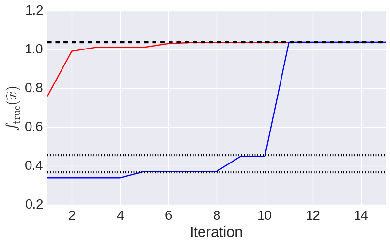
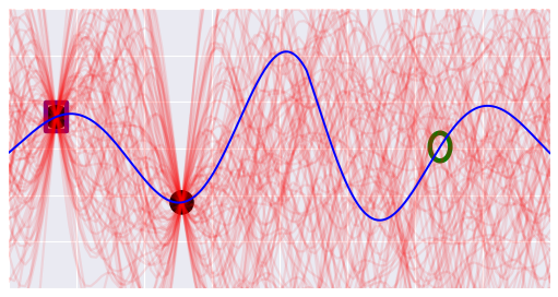
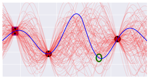
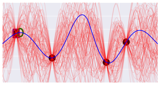
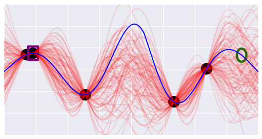
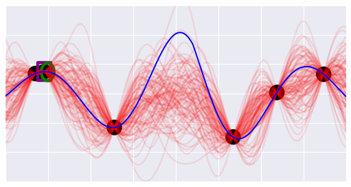
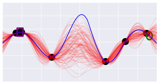
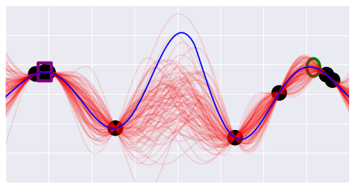
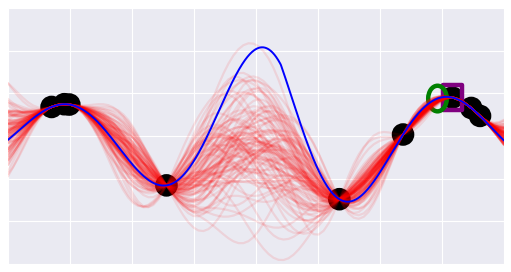
Figure 8: Top: the estimated optimum over time. Blue and Red represent optimization with uniform and Gaussian drift proposals. Black lines indicate the local optima of the true functions. Bottom: a sequence of actions. Depicted are iterations 7-12 with uniform proposals.

In Fig. 8 we show results for our implementation of Bayesian Optimization with Thompson sampling. We compare two different proposal distributions, namely uniform proposals and Gaussian drift proposals. We see that in this experiment, Gaussian drift is starting near the global optimum and drifts quickly towards it. (red curve, top panel of Fig. 8). Uniform proposals take longer to find the global optimum (blue curve, top panel of Fig. 8) but we see that it can surpass the local optima of the curve. The bottom panel of Fig. 8 depicts a sequence of actions using uniform proposals. The sequence illustrates the exploitation exploration trade-off that the implementation overcomes. We start with complete uncertainty ($i=2$). The Bayesian agent performs exploration until it gets a (wrong!) idea of where the optimum could be (exploiting the local optima $i=5$ to $i=10$). $i=11$ shows a change in tactic. The Bayesian agent, having exploited the local optima in previous steps, is now reducing uncertainty in area it knows nothing about, eventually finding the global optimum.

5 Discussion

This paper has shown that it is feasible and useful to embed Gaussian processes in higher-order probabilistic programming languages by treating them as a kind of statistical memoizer. It has described classic GP regression with both fully Bayesian and MAP inference in a hierarchical hyperprior, as well as state-of-the-art applications to discovering symbolic structure in time series and to Bayesian optimization. All the applications share a common 50-line Python GP library and require fewer than 20 lines of probabilistic code each.

These results suggest several research directions. First, it will be important to develop versions of gpmem that are optimized for larger-scale applications. Possible approaches include the standard low-rank approximations to the kernel matrix that are popular in machine learning (Bui and Turner, 2014) as well as more sophisticated sampling algorithms for approximate conditioning of the GP (Lawrence et al., 2009). Second, it seems fruitful to abstract the notion of a “generalizing” memoizer from the specific choice of a Gaussian process model as the mechanism for generalization. “Generalizing” or statistical memoizers with custom regression techniques could be broadly useful in performance engineering and scheduling systems. The timing data from performance benchmarks could be run through a generalizing memoizer by default. This memoizer could be queried (and its output error bars examined) to inform the best strategy for performing the computation or predict the likely runtime of long-running jobs. Third, the structure learning application suggests follow-on research in information retrieval for structured data. It should be possible to build a time series search engine that can handle search predicates such as “has a rising trend starting around 1988” or “is perodic during the 1990s”. The variation on the Automated Statistician presented in this paper can provide ranked result sets for these sorts of queries because it tracks posterior uncertainty over structure and also because the space of structural patterns that it can handle is easy to modify by making small changes to a short VentureScript program.

The field of Bayesian nonparametrics offers a principled, fully Bayesian response to the empirical modeling philosophy in machine learning (Ghahramani, 2012), where Bayesian inference is used to encode a state of broad ignorance rather than a bias stemming from strong prior knowledge. It is perhaps surprising that two key objects from Bayesian nonparametrics, Dirichlet processes and Gaussian processes, fit naturally in probabilistic programming as variants of memoization (Roy et al., 2008). It is not yet clear if the same will be true for other processes, e.g. Wishart processes, or hierarchical Beta processes. We hope that the results in this paper encourage the development of other nonparametric libraries for higher-order probabilistic programming languages.

Acknowledgements

This research was supported by DARPA (under the XDATA and PPAML programs), IARPA (under research contract 2015-15061000003), the Office of Naval Research (under research contract N000141310333), the Army Research Office (under agreement number W911NF-13-1-0212), the Bill & Melinda Gates Foundation, and gifts from Analog Devices and Google.

Appendix

A Covariance Functions

$$k^{\text{se}} =\sigma^{2}\exp(-\frac{(x-x^{\prime})^{2}}{2\ell^{2}})$$ (25)

$$k^{\text{linear}} =\sigma^{2}(xx^{\prime})$$ (26)

$$k^{\text{constant}} =\sigma^{2}$$ (27)

$$k^{\text{wn}} =\sigma^{2}\delta_{x,x^{\prime}}$$ (28)

$$k^{\text{rational quadratic}} =\sigma^{2}\bigg{(}1+\frac{(x-x^{\prime})^{2}}{2\alpha\ell^{2}}\bigg{)}^{-\alpha}$$ (29)

$$k^{\text{periodic}} =\sigma^{2}\exp\bigg{(}\frac{2\sin^{2}(\pi(x-x^{\prime})/p}{\ell^{2}}\bigg{)}.$$ (30)

From top to bottom: the squared-exponential covariance function (25), also know as smoothing kernel; the linear kernel (26); the constant kernel (27); the white noise kernel (28); the rational quadratic kernel (29); and the periodic kernel (30).

B Covariance Simplification

⬇

SE $\times$ SE $\rightarrow$ SEΩ{SE,PER,C,WN} $\times$ WN $\rightarrow$ WNΩLIN $+$ LIN $\rightarrow$ LINΩ{SE,PER,C,WN,LIN} $\times$ C $\rightarrow$ {SE,PER,C,WN,LIN}

Rule 1 is derived as follows:

$$\sigma_{c}^{2}\exp(-\frac{(x-x^{\prime})^{2}}{2\ell_{c}^{2}}) =\sigma_{a}^{2}\exp(-\frac{(x-x^{\prime})^{2}}{2\ell_{a}^{2}})\times\sigma_{b}^{2}\exp(-\frac{(x-x^{\prime})^{2}}{2\ell_{b}^{2}})$$ (31)

$$=\sigma_{c}^{2}\exp(-\frac{(x-x^{\prime})^{2}}{2\ell_{a}^{2}})\times\exp(-\frac{(x-x^{\prime})^{2}}{2\ell_{b}^{2}})$$

$$=\sigma_{c}^{2}\exp\bigg{(}-\frac{(x-x^{\prime})^{2}}{2\ell_{a}^{2}}-\frac{(x-x^{\prime})^{2}}{2\ell_{b}^{2}}\bigg{)}$$

$$=\sigma_{c}^{2}\exp\bigg{(}-\frac{(x-x^{\prime})^{2}}{2\ell_{c}^{2}}\bigg{)}$$

For stationary kernels that only depend on the lag vector between $x$ and $x^{\prime}$ it holds that multiplying such a kernel with a WN kernel we get another WN kernel (Rule 2). Take for example the SE kernel:

$$\sigma_{a}^{2}\exp\bigg{(}-\frac{(x-x^{\prime})^{2}}{2\ell_{c}^{2}}\bigg{)}\times\sigma_{b}\delta_{x,x^{\prime}}=\sigma_{a}\sigma_{b}\delta_{x,x^{\prime}}$$ (32)

Rule 3 is derived as follows:

$$\theta_{c}(x\times x^{\prime})=\theta_{a}(x\times x^{\prime})+\theta_{b}(x\times x^{\prime})$$ (33)

Multiplying any kernel with a constant obviously changes only the scale parameter of a kernel (Rule 4).

C The Struct-Operator

$$\text{Struct}(k^{\text{linear}}) =\text{LIN}$$

$$\text{Struct}(k^{\text{periodic}}) =\text{PER}$$

$$\text{Struct}(k^{\text{se}}) =\text{SE}$$

$$\text{Struct}(k^{\text{wn}}) =\text{WN}$$

$$\text{Struct}(k^{\text{linear+periodic}}) =\text{LIN}+\text{PER}$$

$$\text{Struct}(k^{\text{linear}\times\text{periodic}}) =\text{LIN}\times\text{PER}$$

D Glossary

$\mathcal{N}$	(Multivariate-) Gaussian
$\mathcal{GP}$	Gaussian Process
$\mathbb{E}$	Expectation
$x,x_{i}$	Scalar, possibly indexed with $i$
$\mathbf{x}$	Column vector, training data: regression input (also actions in section 4.3)
$\mathbf{y}$	Column vector, training data: regression output (also rewards in section 4.3)
$\mathcal{X}$	A set of possible actions
$\mathbf{x}^{\prime}$	Column vector, unseen test input: regression input
$\mathbf{y}^{\prime}$	Column vector, sample from predictive posterior, that is a sample from
	$\mathcal{N}(\bm{\mu}_{\bm{\theta}}^{\text{post}},\mathbf{K}_{\bm{\theta}}^{\text{post}})$
$\mathbf{x}^{*}$	Column vector, unseen test input: regression input before any data
	has been observed
$\mathbf{y}^{*}$	Column vector, sample from the predictive prior conditioned on $\bm{\theta}$
	and unseen test input $\mathbf{x}^{*}$
$\mathbf{D}$	Data matrix $[\mathbf{x}\;\mathbf{y}]$
$\mu(x)$	Mean function
$\bm{\theta}_{\text{mean}}$	hyper-parameters for a mean function
$k\text{ or }k(x_{i},x_{j})$	a covariance function or kernel, that is a function that takes two scalars as input
$\bm{\theta}$	hyper-parameters for a kernel/covariacne function (also semicontext in section 4.3)
$k(x_{i},x_{j}\mid\bm{\theta})$	a kernel conditioned on its hyper-parameters
$K(\mathbf{x},\mathbf{x}^{\prime}\mid\bm{\theta})$	Function outputting a matrix of dimension $I\times J$ with entries $k(x_{i},x_{j}\mid\bm{\theta})$;
	with $x_{i}\in\mathbf{x}$ and $x_{j}\in\mathbf{x}^{\prime}$ where $I$ and $J$ indicate the length of the
	column vectors $\mathbf{x}$ and $\mathbf{x}^{\prime}$
$k_{\bm{\theta}}$	a covariance function parameterized with $\bm{\theta}$
$\mathbf{K}_{\bm{\theta}}\text{ or }\mathbf{K}_{(\bm{\theta},\mathbf{x},\mathbf{x})}$	covariance matrix computed with by $K(\mathbf{x},\mathbf{x}\mid\bm{\theta})$
$\bm{\mu}_{\bm{\theta}}^{\text{post}}$	Posterior mean vector for $\mathbf{y}^{\prime}\mid\mathbf{x},\mathbf{x}^{\prime},\mathbf{y},\bm{\theta}$
$\mathbf{K}_{\bm{\theta}}^{\text{post}}$	Posterior covariance matrix for $\mathbf{y}^{\prime}\mid\mathbf{x},\mathbf{x}^{\prime},\mathbf{y},\bm{\theta}$
$\mathbf{L}$	lower triangular matrix, given by the Cholesky factorization as $\mathbf{L}\coloneqq\text{chol}(\mathbf{K}_{\bm{\theta}})$
$k^{\text{se}}$	Squared exponential covariance function
$k^{\text{linear}}$	Linear covariance function
$k^{\text{constant}}$	Constant covariance function
$k^{\text{wn}}$	White noise covariance function
$k^{\text{rational quadratic}}$	Rational quadratic covariance function
$k^{\text{periodic}}$	Periodic covariance function
SE	Symbolic expression for the squared exponential covariance function
LIN	Symbolic expression for the linear covariance function
PER	Symbolic expression for the periodic covariance function
RQ	Symbolic expression for the rational quadratic covariance function
C	Symbolic expression for the constant covariance function
WN	Symbolic expression for the white noise covariance function

$\land$	Logical and
$\lor$	Logical or
$\bm{\mathcal{K}}$	Random variable over kernel functions
kernel functions
Parse$(k)$	Parse the structure for kernel $k$
Simplify$(k)$	Simplify the functional expression for kernel $k$
Struct$(k)$	Symbolic interpretation for kernel $k$
$\text{Contains}(k,k^{t})$	A kernel $k^{t}$ contains the global kernel structure $k$
$\text{SE}(\bm{\mathcal{K}})$	Operator to check if $\text{Struct}(\bm{\mathcal{K}}=k)=\text{SE}$
$\text{LIN}(\bm{\mathcal{K}})$	Operator to check if $\text{Struct}(\bm{\mathcal{K}}=k)=\text{LIN}$
$\text{PER}(\bm{\mathcal{K}})$	Operator to check if $\text{Struct}(\bm{\mathcal{K}}=k)=\text{PER}$
$\text{WN}(\bm{\mathcal{K}})$	Operator to check if $\text{Struct}(\bm{\mathcal{K}}=k)=\text{WN}$
BK	A set of base kernels
$\mathbf{S}$	A subset of BK, randomly selected
$\bm{\Omega}$	Random variable for composition operators, in our case that is kernel addition
	and multiplication $\{+,\times\}$
$\Gamma(\alpha,\beta)$	Gamma distribution with shape parameter $\alpha$ and rate $\beta$
$\ell$	Length-scale parameter for $k^{\text{se}}$
$sf$	Scale factor parameter
$\vartheta\in\Theta$	Context in Thompson sampling
$\Theta$	Context space
$V$	Value function
$Q_{\textrm{proposal}}$	Proposal distribution
$E$	Energy function
$s$	Temperature parameter

References

- Barnett and Barnett (1979) Stephen Barnett and Stephen Barnett. Matrix methods for engineers and scientists. McGraw-Hill, 1979.
- Barry (1986) D. Barry. Nonparametric bayesian regression. The Annals of Statistics, 14(3):934–953, 1986.
- Box et al. (1997) G. E. P. Box, G. M. Jenkins, and G. C. Reinsel. Time series analysis: forecasting and control. 1997.
- Bui and Turner (2014) T. D. Bui and R. E. Turner. Tree-structured gaussian process approximations. In Advances in Neural Information Processing Systems, pages 2213–2221, 2014.
- Damianou and Lawrence (2013) A. Damianou and N. Lawrence. Deep gaussian processes. In Proceedings of the International Conference on Artificial Intelligence and Statistics (AISTATS), pages 207–215, 2013.
- Duvenaud et al. (2013) D. Duvenaud, J. R. Lloyd, R. Grosse, J. Tenenbaum, and Z. Ghahramani. Structure discovery in nonparametric regression through compositional kernel search. In Proceedings of the International Conference on Machine Learning (ICML), pages 1166–1174, 2013.
- Ferris et al. (2006) B. Ferris, D. Haehnel, and D. Fox. Gaussian processes for signal strength-based location estimation. In Proceedings of the Conference on Robotics Science and Systems. Citeseer, 2006.
- Gelbart et al. (2014) M. A. Gelbart, J. Snoek, and R. P. Adams. Bayesian optimization with unknown constraints. arXiv preprint arXiv:1403.5607, 2014.
- Ghahramani (2012) Z. Ghahramani. Bayesian non-parametrics and the probabilistic approach to modelling. Philosophical Transactions of the Royal Society of London A: Mathematical, Physical and Engineering Sciences, 371(1984):20110553, 2012.
- Kemmler et al. (2013) M. Kemmler, E. Rodner, E. Wacker, and J. Denzler. One-class classification with gaussian processes. Pattern Recognition, 46(12):3507–3518, 2013.
- Kennedy and O’Hagan (2001) M. C. Kennedy and A. O’Hagan. Bayesian calibration of computer models. Journal of the Royal Statistical Society. Series B, Statistical Methodology, pages 425–464, 2001.
- Kuss and Rasmussen (2005) M. Kuss and C. E. Rasmussen. Assessing approximate inference for binary gaussian process classification. The Journal of Machine Learning Research, 6:1679–1704, 2005.
- Kwan et al. (2013) J. Kwan, S. Bhattacharya, K. Heitmann, and S. Habib. Cosmic emulation: The concentration-mass relation for wcdm universes. The Astrophysical Journal, 768(2):123, 2013.
- Lawrence et al. (2009) N. D. Lawrence, M. Rattray, and M. K. Titsias. Efficient sampling for gaussian process inference using control variables. In Advances in Neural Information Processing Systems, pages 1681–1688, 2009.
- Lloyd et al. (2014) J. R. Lloyd, D. Duvenaud, R. Grosse, J. Tenenbaum, and Z. Ghahramani. Automatic construction and natural-language description of nonparametric regression models. In Proceedings of the Conference on Artificial Intelligence (AAAI), 2014.
- MacKay (1998) David JC MacKay. Introduction to gaussian processes. NATO ASI Series F Computer and Systems Sciences, 168:133–166, 1998.
- Mansinghka et al. (2014) V. K. Mansinghka, D. Selsam, and Y. Perov. Venture: a higher-order probabilistic programming platform with programmable inference. arXiv preprint arXiv:1404.0099, 2014.
- Neal (1995) R. M. Neal. Bayesian Learning for Neural Networks. PhD thesis, University of Toronto, 1995.
- Neal (1997) R. M. Neal. Monte carlo implementation of gaussian process models for bayesian regression and classification. arXiv preprint physics/9701026, 1997.
- Rasmussen and Williams (2006) C. E. Rasmussen and C. K. I. Williams. Gaussian Processes for Machine Learning (Adaptive Computation and Machine Learning). The MIT Press, 2006.
- Roy et al. (2008) D. M. Roy, V. K. Mansinghka, N. D. Goodman, and J. B. Tenenbaum. A stochastic programming perspective on nonparametric bayes. In Nonparametric Bayesian Workshop, Int. Conf. on Machine Learning, volume 22, page 26, 2008.
- Schneider et al. (2008) M. D. Schneider, L. Knox, S. Habib, K. Heitmann, D. Higdon, and C. Nakhleh. Simulations and cosmological inference: A statistical model for power spectra means and covariances. Physical Review D, 78(6):063529, 2008.
- Snoek et al. (2012) J. Snoek, H. Larochelle, and R. P. Adams. Practical bayesian optimization of machine learning algorithms. In Advances in Neural Information Processing Systems (NIPS), pages 2951–2959, 2012.
- The GPy authors (2012–2015) The GPy authors. GPy: A gaussian process framework in python. http://github.com/SheffieldML/GPy, 2012–2015.
- Thompson (1933) W. R. Thompson. On the likelihood that one unknown probability exceeds another in view of the evidence of two samples. Biometrika, pages 285–294, 1933.
- Williams and Barber (1998) C. K. I. Williams and D. Barber. Bayesian classification with gaussian processes. IEEE Transactions on Pattern Analysis and Machine Intelligence, 20(12):1342–1351, 1998.