Signal Representations on Graphs: Tools and Applications
Abstract
We present a framework for representing and modeling data on graphs. Based on this framework, we study three typical classes of graph signals: smooth graph signals, piecewise-constant graph signals, and piecewise-smooth graph signals. For each class, we provide an explicit definition of the graph signals and construct a corresponding graph dictionary with desirable properties. We then study how such graph dictionary works in two standard tasks: approximation and sampling followed with recovery, both from theoretical as well as algorithmic perspectives. Finally, for each class, we present a case study of a real-world problem by using the proposed methodology.
Index Terms:
Discrete signal processing on graphs, signal representationsI Introduction
Signal processing on graphs is a framework that extends classical discrete signal processing to signals with an underlying complex and irregular structure. The framework models that underlying structure by a graph and signals by graph signals, generalizing concepts and tools from classical discrete signal processing to graph signal processing. Recent work includes graph-based transforms [1, 2, 3], sampling and interpolation on graphs [4, 5, 6], graph signal recovery [7, 8, 9, 10], uncertainty principle on graphs [11, 12], graph dictionary learning [13, 14], community detection [15, 16, 17] , and many others.
In this paper, we consider the signal representations on graphs. Signal representation is one of the most fundamental tasks in our discipline. For example, in classical signal processing, we use the Fourier basis to represent the sine waves; we use the wavelet basis to represent smooth signals with transition changes. Signal representation is highly related to approximation, compression, denoising, inpainting, detection, and localization [18, 19]. Previous works along those lines consider representations based on the graph Fourier domain, which emphasize the smoothness and global behavior of a graph signal [20], as well as the representations based on the graph vertex domain, which emphasize the connectivity and localization of a graph signal [21, 22].
We start by proposing a representation-based framework, which provides a recipe to model real-world data on graphs. Based on this framework, we study three typical classes of graph signals: smooth graph signals, piecewise-constant graph signals, and piecewise-smooth graph signals. For each class, we provide an explicit definition for the graph signals and construct a corresponding graph dictionary with desirable properties. We then study how the proposed graph dictionary works in two standard tasks: approximation and sampling followed with recovery, both from theoretical as well as algorithmic perspectives. Finally, for each class, we present a case study of a real-world problem by using the proposed methodology.
Contributions. The main contribution of this paper is to build a novel and unified framework to analyze graph signals. The framework provides a general solution allowing us to study real-world data on graphs. Based on the framework, we study three typical classes of graph signals:
-
•
Smooth graph signals. We explicitly define the smoothness criterion and construct corresponding representation dictionaries. We propose a generalized uncertainty principle on graphs and study the localization phenomenon of graph Fourier bases. We then investigate how the proposed graph dictionary works in approximation and sampling followed with recovery. Finally, we demonstrate a case study on a co-authorship network.
-
•
Piecewise-constant graph signals. We explicitly define piecewise-constant graph signals and construct the multiresolution local sets, a local-set-based piecewise-constant dictionary and local-set-based piecewise-constant wavelet basis, which provide a multiresolution analysis on graphs and promote sparsity for such graph signals. We then investigate how the proposed local-set-based piecewise-constant dictionary works for approximation and sampling followed with recovery. Finally, we demonstrate a case study on epidemics processes.
-
•
Piecewise-smooth graph signals. We explicitly define piecewise-smooth graph signals and construct a local-set-based piecewise-smooth dictionary, which promotes sparsity for such graph signals. We then investigate how the proposed local-set-based piecewise-smooth dictionary works in approximation. Finally, we demonstrate a case study on environmental change detection.
Outline of the paper. Section II introduces and reviews the background on signal processing on graphs; Section III proposes a representation-based framework to study graph signals, which lays the foundation for this paper; Sections IV, V, and VI present representations of smooth, piecewise constant, and piecewise smooth graph signals, respectively, including their effectiveness in approximation and sampling followed by recovery, as well as validation on three different real-world problems: co-authorship network, epidemics processes, and environmental change detection. Section VII concludes the paper.
II Signal Processing on Graphs
Let be a directed, irregular and weighted graph, where is the set of nodes, is the set of weighted edges, and is the weighted adjacency matrix, whose element measures the underlying relation between the th and the th nodes. Let be a degree vector, where . Given a fixed ordering of nodes, we assign a signal coefficient to each node; a graph signal is then defined as a vector,
with the signal coefficient corresponding to the node .
To represent the graph structure by a matrix, two basic approaches have been considered. The first one is based on algebraic signal processing [23], and is the one we follow. We use the graph shift operator as a graph representation, which is an elementary filtering operation that replaces a signal coefficient at a node with a weighted linear combination of coefficients at its neighboring nodes. Some common choices of a graph shift are weighted adjacency matrix , normalized adjacency matrix , and transition matrix [24]. The second one is based on the spectral graph theory [25], where the graph Laplacian matrix is used as a graph representation, which is a second-order difference operator on graphs. Some common choices of a graph Laplacian matrix are the unnormalized Laplacian , the normalized Laplacian , and the transition Laplacian .
| Graph shift | Graph Laplacian | |
|---|---|---|
| Unnormalized | ||
| Normalized | ||
| Transition |
A graph shift emphasizes the similarity while a graph Laplacian matrix emphasizes the difference between each pair of nodes. The graph shift and graph Laplacian matrix often appear in pairs; see Table I. Another overview is presented in [26]. We use to represent a graph structure matrix, which can be either a graph shift or a graph Laplacian matrix. Based on this graph structure matrix, we are able to generalize many tools from traditional signal processing to graphs, including filtering [27, 28], Fourier transform [29, 1], wavelet transforms [30, 2], and many others. We now briefly review the graph Fourier transform.
The graph Fourier basis generalizes the traditional Fourier basis and is used to represent the graph signal in the graph spectral domain. The graph Fourier basis is defined to be the eigenvector matrix of , that is,
where the th column vector of is the graph Fourier basis vector corresponding to the eigenvalue as the th diagonal element in . The graph Fourier transform of is where is called the graph Fourier transform matrix. When is symmetric, then is orthornormal; the graph Fourier basis vector is the th row vector of . The inverse graph Fourier transform is The vector represents the frequency coefficients corresponding to the graph signal , and the graph Fourier basis vectors can be regarded as graph frequency components. In this paper, we use , to denote the inverse graph Fourier transform matrix and graph Fourier transform matrix for a general graph structure matrix, which can be an adjacency matrix, a graph Laplacian, or a transition matrix. When we emphasize that and is generated from a certain graph structure matrix, we add a subscript. For example, is the graph Fourier transform matrix of the weighted adjacency matrix .
The ordering of graph Fourier basis vectors depends on their variations. The variations of a graph signal are defined in different ways. When the graph representation matrix is the graph shift, the variation of a graph signal is defined as,
where is the eigenvalue of with the largest magnitude. We can show that when the eigenvalues of the graph shift are sorted in a nonincreasing order , the variations of the corresponding eigenvectors follow a nondecreasing order .
When the graph representation matrix is the graph Laplacian matrix, the variation of a graph signal is defined as,
Similarly, we can show that when the eigenvalues of the graph Laplacian are sorted in a nondecreasing order , the variations of the corresponding eigenvectors follows a nondecreasing order .
The variations of graph Fourier basis vectors thus allow us to provide the ordering: the Fourier basis vectors with small variations are considered as low-frequency components while the vectors with large variations are considered as high-frequency components [31]. We will discuss the difference between these two variations in Section IV.
Based on the above discussion, the eigenvectors associated with large eigenvalues of the graph shift (small eigenvalues of the graph Laplacian) represent low-frequency components and the eigenvectors associated with small eigenvalues of the graph shift (large eigenvalues of graph Laplacian) represent high-frequency components. In the following discussion, we assume all graph Fourier bases are ordered from low frequencies to high frequencies.
III Foundations
In this section, we introduce a representation-based framework with three components, including graph signal models, representation dictionaries and the related tasks, in a general and abstract level. This lays a foundation for the following sections, which are essentially special cases that follow this general framework.
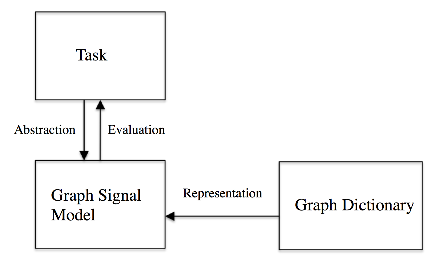 |
As shown in Figure 1, when studying a task with a graph, we first model the given data with some graph signal model. The model describes data by capturing its important properties. Those properties can be obtained from observations, domain knowledge, or statistical learning algorithms. We then use a representation dictionary to represent the graph signal model. In the following discussion, we go through each component one by one.
III-A Graph Signal Model
In classical signal processing, people often work with signals with some specific properties, instead of arbitrary signals. For example, smooth signals have been studied extensively over decades; sparse signals are intensively studied recently. Here we also need a graph signal model to describe a class of graph signals with specific properties. In general, there are two approaches to mathematically model a graph signal, including a descriptive approach and a generative approach.
For the descriptive approach, we describe the properties of a graph signal by bounding the output of some operator. Let be a graph signal, be a function operating on , we define a class of graph signals by restricting
| (1) |
where is some constant. For example, we define smooth graph signals by restricting be small [32].
For the generative approach, we describe the properties of a graph signal by using a graph dictionary. Let be a graph dictionary, we define a class of graph signals by restricting
where is a vector of expansion coefficients. For the descriptive approach, we do not need to know everything about a graph signal, instead, we just need to its output of some operator; for the generative approach, we need to reconstruct a graph signal, which requires to know everything about a graph signal.
III-B Graph Dictionary
For a certain graph signal model, we aim to find some dictionary to provide accurate and concise representations.
III-B1 Design
In general, there are two approaches to design a graph dictionary, including a passive approach and a active one.
For the passive approach, the graph dictionary is designed only based on the graph structure; that is,
where is some operator on the graph structure matrix . For example, can be the eigenvector matrix of , which is the graph Fourier basis. In classical signal processing, the Fourier basis, wavelet bases, wavelet frames, and Gabor frames are all constructed using this approach, where the graph is a line graph or a lattice graph [23].
For the active approach, the graph dictionary is designed based on both graph structure and a set of given graph signals; that is,
where is a matrix representation of a set of graph signals. We can fit to those given graph signals and provide a specialized dictionary. Some related works see [13, 14].
III-B2 Properties
The same class of graph signals can be modeled by various dictionaries. For example, whenever is an identity matrix, it can represent arbitrary graph signals, but may not be appealing to represent a non-sparse signals. Depending on the application, we may have different requirements for the constructed graph dictionary. Here are some standard properties of a graph dictionary , we aim to study.
-
•
Frame bounds. For any in a certain graph signal model,
where are some constants;
-
•
Sparse representations. For any in a certain graph signal model, there exists a sparse coefficient with , which satisfies
where are some constants;
-
•
Uncertainty principles. For any in a certain graph signal model, the following is satisfied
where and , and .
III-C Graph Signal Processing Tasks
We mainly consider two standard tasks in signal processing, approximation and sampling followed with recovery.
III-C1 Approximation
Approximation is a standard task to evaluate a representation. The goal is to use a few expansion coefficients to approximate a graph signal. We consider approximating a graph signal by using a linear combination of a few atoms from and solving the following sparse coding problem,
where is some evaluation metric. The objective function measures the difference between the original signal and the approximated one, which evaluates how well the designed graph dictionary represents a given graph signal. The same formulation can also be used for denoising graph signals.
III-C2 Sampling and Recovery
The goal is to recover an original graph signal from a few samples. We consider a general sampling and recovery setting. We consider any decrease in dimension via a linear operator as sampling, and, conversely, any increase in dimension via a linear operator as recovery [19]. Let be a sampling pattern matrix, which is constrained by a given application and the sampling operator is
| (3) |
where selects rows from . For example, when we choose the th row of as the th sample, the th row of is
There are three sampling strategies: (1) uniform sampling when designing , , where row indices are chosen from from independently and uniformly; and experimentally design sampling, where row indices can be chosen beforehand; and active sampling, where we will use feedback as samples are sequentially collected to decide the next row to be sampled. Each sampling strategy can be implemented by two approaches, including a random approach and a deterministic one. The sampling pattern matrix constraints the following sampling patterns: when is an identity matrix, is a subsampling operator; when is a Gaussian random matrix, is a compressed sampling operator.
In the sampling phase, we take samples with the sampling operator ,
is a vector of samples and is noise with zero mean and as variance. In the recovery phase, we reconstruct the graph signal by using a recovery operator ,
where recovers either exactly or approximately. The evaluation metric can be the mean square error or other metrics. Without any property of , it is hopeless to design an efficient sampling and recovery strategy. Here we focus on a special graph signal model, which can be described by a graph dictionary. The prototype of designing sampling and recovery strategies is
where is some evaluation metric. The optimal sampling and recovery strategies are influenced by the given graph dictionary . We often consider fixing either the sampling strategy or the recovery strategy and optimizing over the other one.
IV Representations of Smooth Graph Signals
Smooth graph signals are mostly studied in the previous literature; however, many works only provide a heuristic. Here we rigorously define graph signal models and design the corresponding graph dictionaries.
 |
 |
 |
 |
| (a) . | (b) . | (c) . | (d) . |
 |
 |
 |
 |
| (e) . | (f) . | (g) . | (h) . |
 |
 |
 |
 |
| (i) . | (j) . | (k) . | (l) . |
IV-A Graph Signal Models
We introduce four smoothness criteria for graph signals; while they have been implicitly mentioned previously, none have been rigorously defined. The goal here is not to conclude which criterion or representation approach works best; instead, we aim to study the properties of various smoothness criteria and model a smooth graph signal with a proper criterion.
We start with the pairwise Lipschitz smooth criterion.
Definition 1.
A graph signal with unit norm is pairwise Lipschitz smooth with parameter when it satisfies
with the distance between the th and the th nodes.
We can choose the geodesic distance, the diffusion distance [33], or some other distance metric for . Similarly to the traditional Lipschitz criterion [18], the pairwise Lipschitz smoothness criterion emphasizes pairwise smoothness, which zooms into the difference between each pair of adjacent nodes.
Definition 2.
A graph signal with unit norm is total Lipschitz smooth with parameter when it satisfies
The total Lipschitz smoothness criterion generalizes the pairwise Lipschitz smoothness criterion while still emphasizing pairwise smoothness, but in a less restricted manner; it is also known as the Laplacian smoothness criterion [34].
Definition 3.
A graph signal with unit norm is local normalized neighboring smooth with parameter when it satisfies
The local normalized neighboring smoothness criterion compares each node to the local normalized average of its immediate neighbors.
Definition 4.
A graph signal with unit norm is global normalized neighboring smooth with parameter when it satisfies
The global normalized neighboring smoothness criterion compares each node to the global normalized average of its immediate neighbors. The difference between the local normalized neighboring smoothness criterion and the global normalized neighboring smoothness criterion is the normalization factor. For the local normalized neighboring smoothness criterion, each node has its own normalization factor; for the global normalized neighboring smoothness criterion, all nodes have the same normalization factor.
The four criteria quantify smoothness in different ways: the pairwise and the total Lipschitz ones focus on the variation of two signal coefficients connected by an edge with the pairwise Lipschitz one more restricted, while the local and global neighboring smoothness criterion focuses on comparing a node to the average of its neighbors.
IV-B Graph Dictionary
As shown in (1), The graph signal models in Definitions 1, 2, 3, 4 are introduced in a descriptive approach. Following these, we are going to translate the descriptive approach into a generative approach; that is, we represent the corresponding signal classes satisfying each of the four criteria by some representation graph dictionary.
IV-B1 Design
We first construct polynomial graph signals that satisfy the Lipschitz smoothness criterion.
Definition 5.
A graph signal is polynomial with degree when
where and is a graph polynomial dictionary with . Denote this class by .
 |
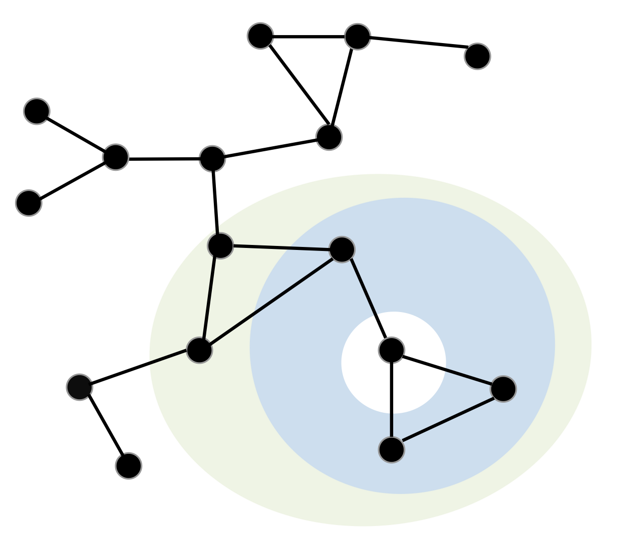 |
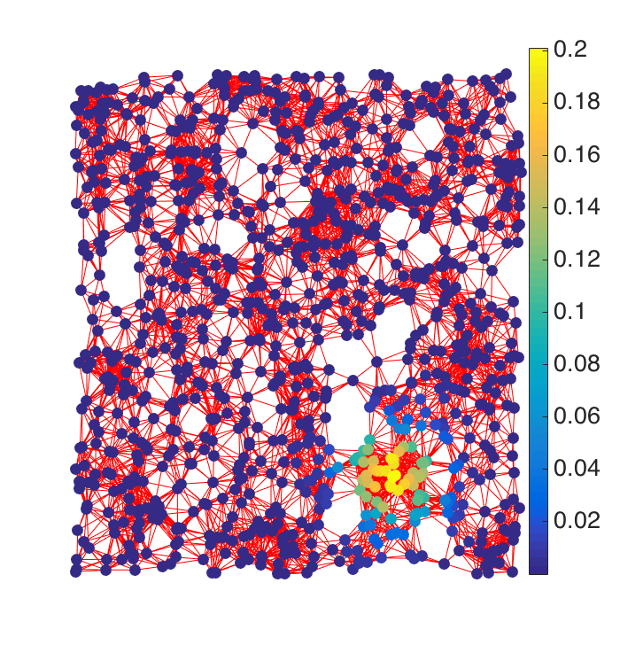
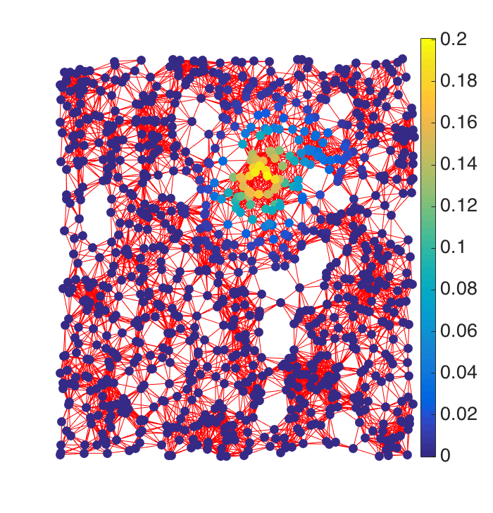
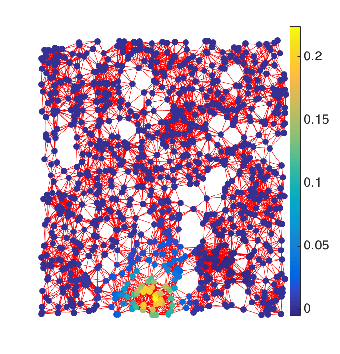
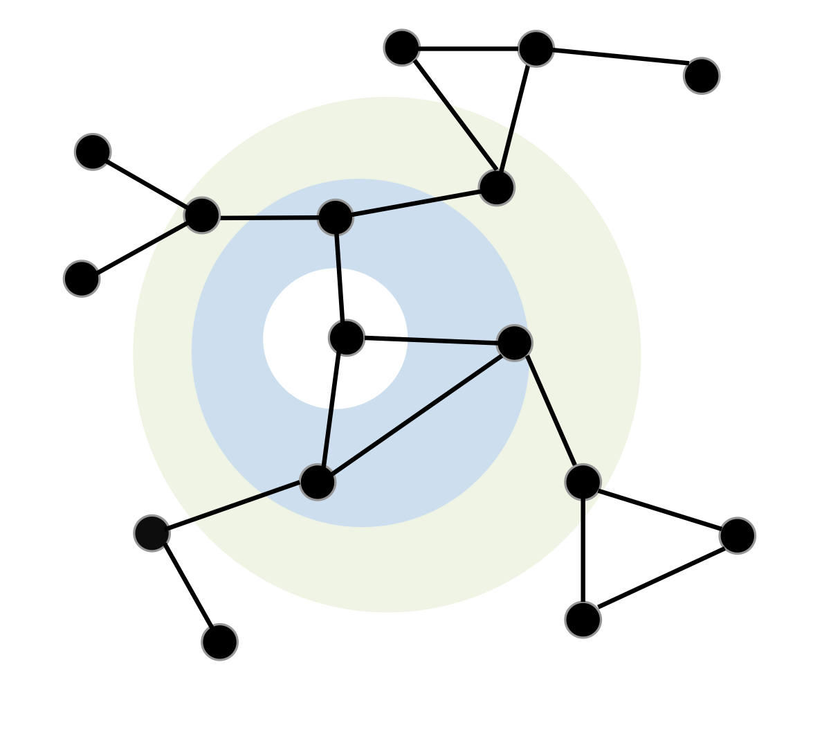
In classical signal processing, polynomial time signals can be expressed as , ; we can rewrite this as in the above definition as , with . The columns of are denoted as , , and called atoms; the elements of each atom are . Since polynomial time signals are shift-invariant, we can set any time point as the origin; such signals are thus characterized by degrees of freedom , . This is not true for graph signals, however; they are not shift-invariant and any node can serve as the origin (see Figure 3). In the above definition, are now matrices with the number of atoms equal to the number of nodes (with each atom corresponding to the node serving as the origin). The dictionary thus contains atoms.
Theorem 1.
(Graph polynomial dictionary represents the pairwise Lipschiz smooth signals) is a subset of the pairwise Lipschitz smooth with some parameter .
Proof.
Let , that is,
Then, we write the pairwise Lipschitz smooth criterion as
The parameter , which corresponds to the energy of the original graph signal. ∎
We now construct bandlimited signals that satisfy the total Lipschitz, local normalized neighboring and global normalized neighboring smoothness smoothness criteria.
Definition 6.
A graph signal is bandlimited with respect to a graph Fourier basis with bandwidth when
where and is a submatrix containing the first columns of . Denote this class by [10].
When is the eigenvector matrix of the unnormalized graph Laplacian matrix, we denote it as and can show that signals in are total Lipschitz smooth; when is the eigenvector matrix of the transition matrix, we denote it as and can show that signals in are local normalized neighboring smooth; when is the eigenvector matrix of the weighted adjacency matrix, we denote it as and can show that signals in are global normalized neighboring smooth.
Theorem 2.
(The graph Fourier basis of the graph Laplacian represents the total Lipschiz smooth signals) For any , is a subset of the total Lipschitz smooth with parameter , when .
Proof.
Let be a graph signal with bandwidth , that is,
Then, we write the total Lipschitz smooth criterion as
∎
Theorem 3.
(The graph Fourier basis of the transition matrix represents the local normalized neighboring smooth signals) For any , is a subset of the local normalized neighboring smooth with parameter , when .
Proof.
Let be a graph signal with bandwidth , that is,
Then, we write the local normalized neighboring smooth criterion as
The last equality follows from the fact that and are eigenvectors and eigenvalues of .
∎
Theorem 4.
(The graph Fourier basis of the adjacency matrix represents the global normalized neighboring smooth signals) For any , is a subset of the global normalized neighboring smooth with parameter , when .
The proof is similar to Theorem 3. Note that for graph Laplacian, the eigenvalues are sorted in an ascending order; for the transition matrix and the adjacency matrix, the eigenvalues are sorted in a descending order.
Each of these three models generates smooth graph signals according to one of the four criteria in Definitions 1, 2, 3 and 4: models Lipschitz smooth signals; models total Lipschitz smooth signals; with models the local normalized neighboring smooth signals; and models the global normalized neighboring smooth signals; the corresponding graph representation dictionaries are , , , and .
IV-B2 Properties
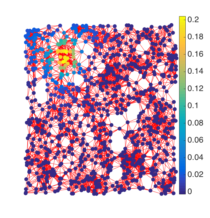
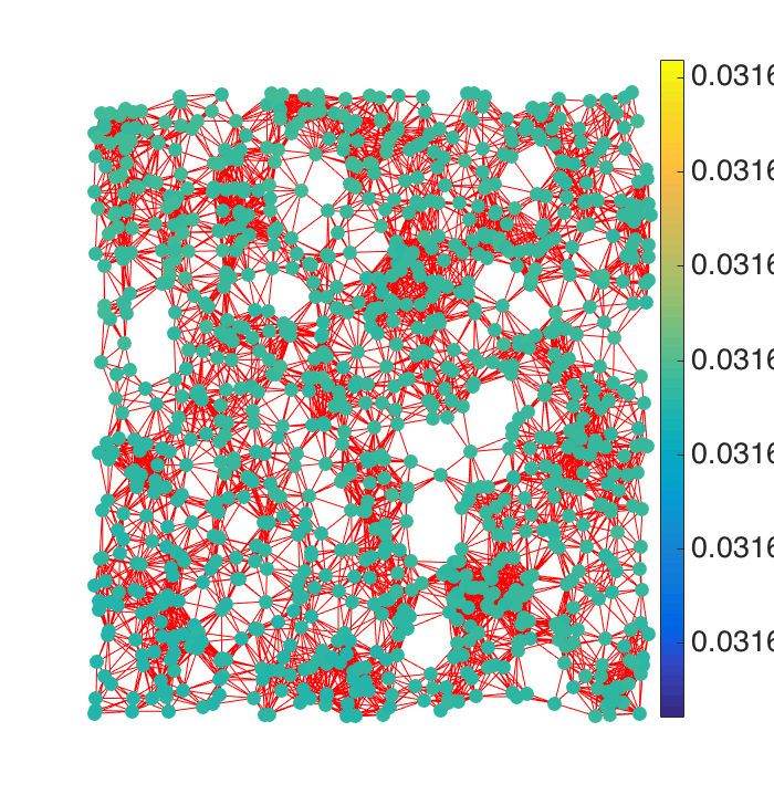
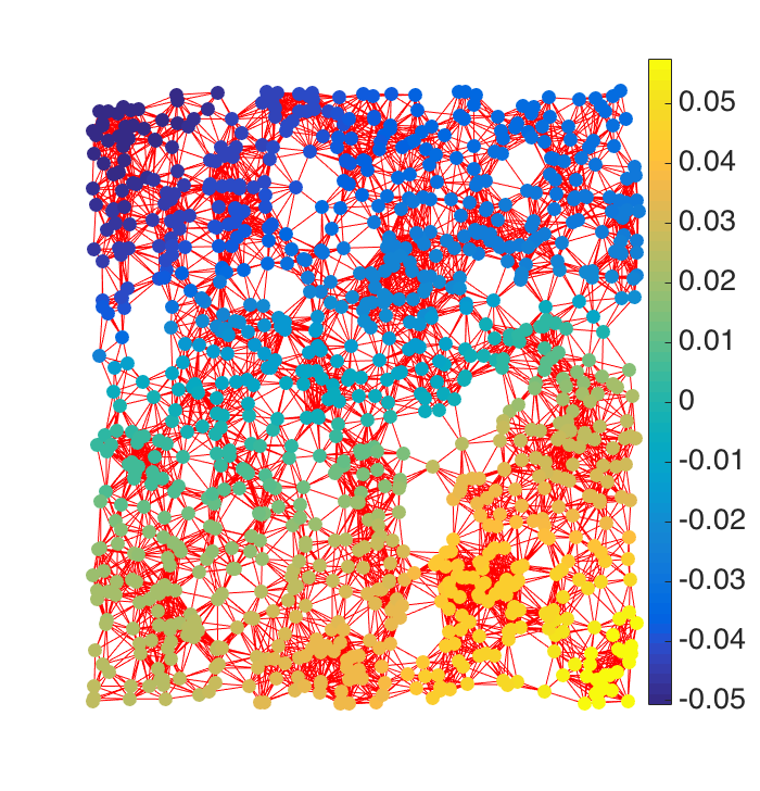
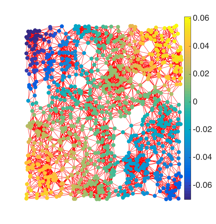
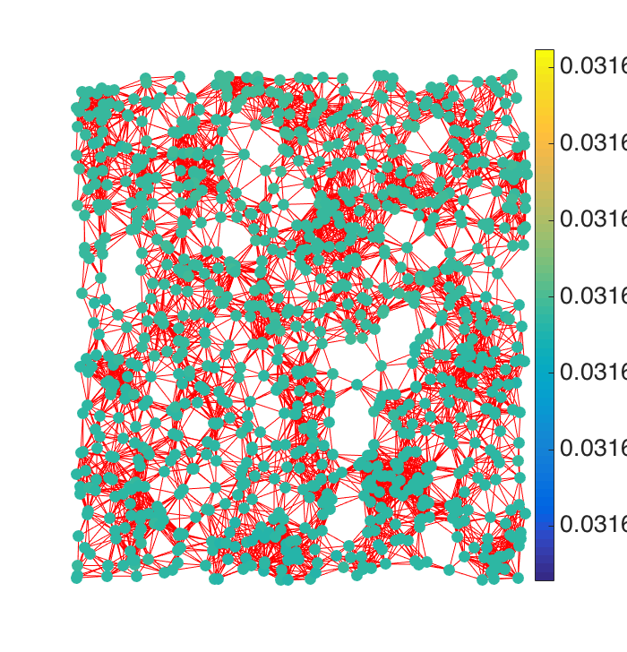
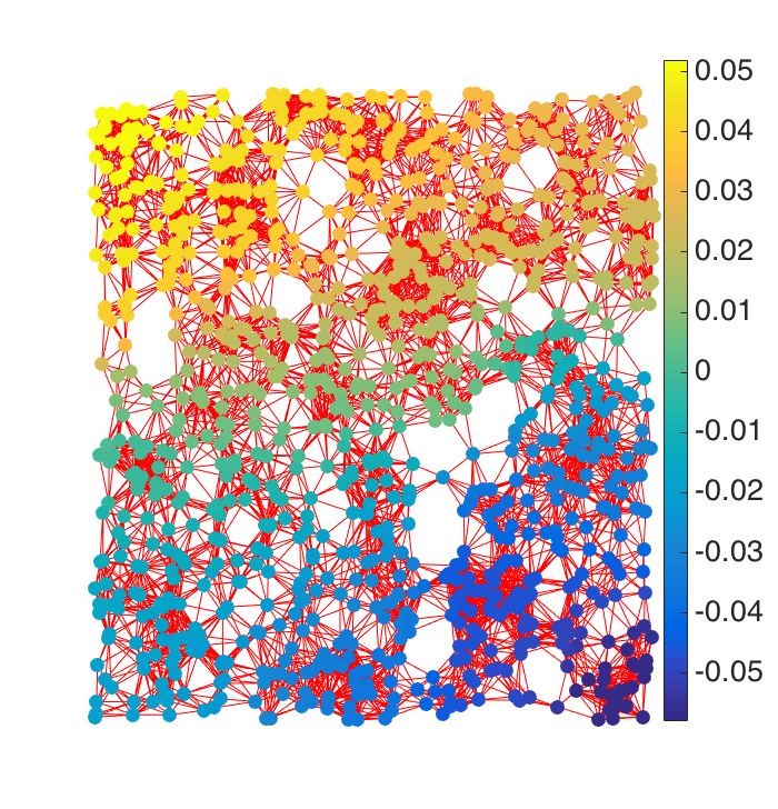
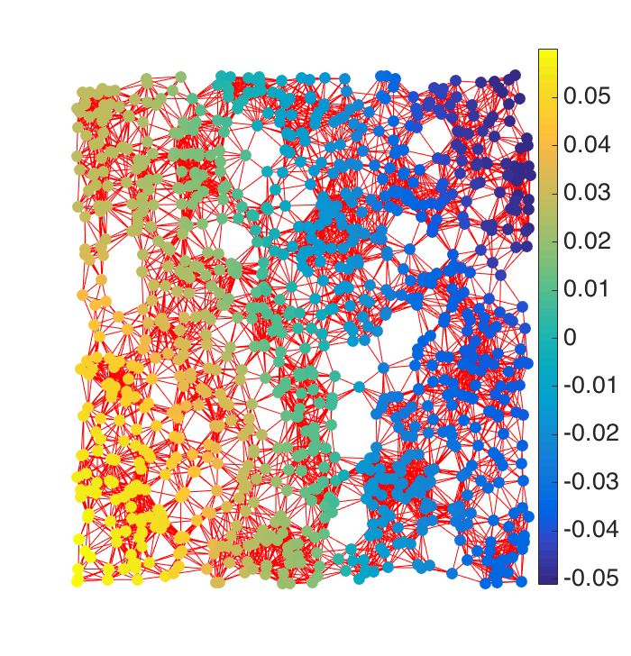
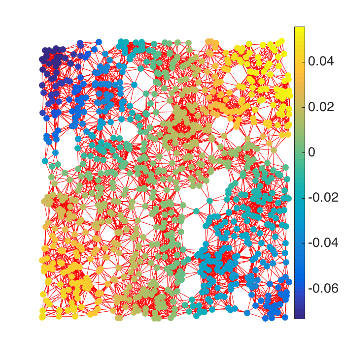
We next study the properties of graph representation dictionaries for smooth graph signals, especially for graph Fourier bases , , and . We first visualize them in Figures 2. Figure 2 compares the first four graph Fourier basis vectors of , and in a geometric graph. We see that tends to localize in some small regions; and have similar behaviors.
We then check the properties mentioned in Section III-B2.
Frame Bound. Graph polynomial dictionary is highly redundant and the frame bound is loose. When the graph is undirected, the adjacency matrix is symmetric, then and are orthonormal. It is hard to draw any meaningful conclusion when the graph is directed; we leave it for the future work.
Sparse Representations. Graph polynomial dictionary provides sparse representations for polynomial graph signals. On the other hand, the graph Fourier bases provide sparse representations for the bandlimited graph signals. For approximately bandlimited graph signals, there are some residuals coming from the high-frequency components.
Uncertainty Principles. In classical signal processing, it is well known that signals cannot localize in both time and frequency domains at the same time [19, 35]. Some previous works extend this uncertainty principle to graphs by studying how well a graph signal exactly localize in both the graph vertex and graph spectrum domain [11, 12]. Here we study how well a graph signal approximately localize in both the graph vertex and graph spectrum domain. We will see that the localization depends on the graph Fourier basis.
Definition 7.
A graph signal is -vertex concentrated on a graph vertex set when it satisfies
where is a diagonal matrix, with when and , otherwise.
The vertex set represents a region that supports the main energy of signals. When is small, a -vertex concentrated signal is approximately sparse.
Definition 8.
A graph signal is -spectrum concentrated on a graph spectrum band when it satisfies
where is a submatrix of with columns selected by and is a submatrix of with rows selected by .
The graph spectrum band provides a bandlimited space that supports the main energy of signals. An equivalent formulation is . Definition 8 is a simpler version of the approximately bandlimited space in [6].
Theorem 5.
(Uncertainty principle of the graph vertex and spectrum domains) Let a unit norm signal supported on an undirected graph be -vertex concentrated and -spectrum concentrated at the same time. Then,
Proof.
We first show .
where
Let be a graph signal with . Then, . We then have
We then show that . Based on the assumption, we have
Since has a unit norm, by the triangle inequality, we have
Finally, we combine two results and obtain
∎
We see that the lower bound involves with the maximum magnitude of . In classical signal processing, is the discrete Fourier transform matrix, so ; the lower bound is and signals cannot localize in both time and frequency domain. However, for complex and irregular graphs, the energy of a graph Fourier basis vector may concentrate on a few elements, that is, , as shown in Figures 2(a)(b)(c)(d). It is thus possible that graph signals can be localized in both the vertex and spectrum domain. We now illustrate this localization phenomenon
Localization Phenomenon. A part of this section has been shown in [36]. We show it here for the completeness. The localization of a graph signal means that most elements in a graph signal are zeros, or have small values; only a small number of elements have large magnitudes and the corresponding nodes are clustered in one subgraph with a small diameter.
Prior work uses inverse participation ratio (IPR) to quantify localization [37]. The IPR of a graph signal is
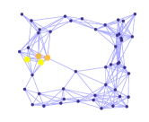
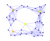
A large IPR indicates that is localized, while a small IPR indicates that is not localized. The range of IPR is from to . For example, is the most delocalized vector with , while is the most localized vector with . IPR has some shortcomings: a) IPR only promotes sparsity, that is, a high IPR does not necessarily mean that the nonzero elements concentrate in a clustered subgraph, which is the essence of localization (Figure 4); b) IPR does not work well for large-scale datasets. When is large, even if only a small set of elements are non zero, IPR tends to be small.
 |
 |
| (a) clustered graph signal. | (b) unclustered graph signal. |
To solve this, we propose a novel measure to quantify the localization of a graph signal. We use energy concentration ratio (ECR) to quantify the energy concentration property. The ECR is defined as
where is the smallest that satisfies with the first elements with the largest magnitude in . This indicates that 95% energy of a graph signal is concentrated in the first elements with largest magnitude. ECR ranges from 0 to 1: when the signal is energy-concentrated, the ECR is small; when the energy of the signal is evenly distributed, the ECR is 1.
We next use normalized geodesic distance (NGD) to quantify the clustered property. Let be the set of nodes that possesses 95% energy of the whole signal. The normalized geodesic distance is defined as:
where is the diameter of the graph, is the geodesic distance between nodes and . Here we use the normalized average geodesic distance as a measure to determine whether the nodes are highly connected. We use the average geodesic distance instead of the largest geodesic distance to avoid the influence of outliers. The NGD ranges from 0 to 1: when the nodes are clustered in a small subgraph, the NGD is small; when the nodes are dispersive, the NGD is large.
We use ECR and NGD together to determine the localization of graph signals. When the two measures are small, the energy of the signal is concentrated in a small set of highly connected nodes, which can be interpreted as localization.
Each graph Fourier basis vector is regarded as a graph signal. When most basis vectors in the graph Fourier basis are localized, that is, the corresponding ECRs and NGDs are small, we call that graph Fourier basis localized.
We now investigate the localization phenomenon of graph Fourier bases of several real-world networks, including the arXiv general relativity and quantum cosmology (GrQc) collaboration network [38], arXiv High Energy Physics - Theory (Hep-Th) collaboration network [38] and the Facebook ‘friend circles’ network [38]. We find similar localization phenomena among different datasets. Due to the limited space, we only show the result of arXiv GrQc collaboration network. The arXiv GrQc network represents the collaborations between authors based on the submitted papers in general relativity and quantum cosmology category of arXiv. When the author and author coauthored a paper, the graph contains an undirected edge between node and . The graph contains 5242 nodes and 14496 undirected edges. Since the graph is not connected, we choose a connect component with 4158 nodes and 13422 edges.
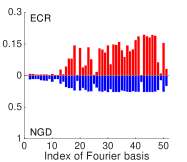
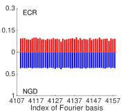
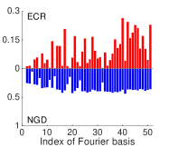
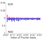
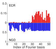
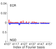
We investigate the Fourier bases of the weighted adjacency matrix, the transition matrix and the unnormalized graph Laplacian matrix in the arXiv GrQc network. Figure 5 illustrates the ECRs and NGDs of the first 50 graph Fourier basis vectors (low-frequency components) and the last 50 graph Fourier basis vectors (high-frequency components) of the three graph representation matrices, where the ECR and NGD are plotted as a function of the index of the corresponding graph Fourier basis vectors. We find that a large number of graph Fourier basis vectors has small ECRs and NGDs, which indicates that graph Fourier basis vectors of various graph representation matrices are localized. Among various graph representation matrices, the graph Fourier basis vectors of graph Laplacian matrix tend to be more localized, especially in high-frequency components. In low-frequency components, the graph Fourier basis vectors of adjacency matrix are more localized.
To combine the uncertainty principle previously, when the graph Fourier basis shows localization phenomenon, it is possible that a graph signal can be localized in both graph vertex and spectrum domain. Based the graph Fourier basis of the graph Laplacian, a high-frequency bandlimited signals can be well localized in the graph vertex domain; based on the graph Fourier basis of adjacency matrix, a low-frequency bandlimited signals can be well localized in the graph vertex domain. The Fourier transform is famous for capturing the global behaviors and works as a counterpart of the delta functions; however, this may not be true on graphs. The study of new role of the graph Fourier transform will be an interesting future work.
| low-frequency components | high-frequency components |
 |
 |
| (a) . | (b) . |
 |
 |
| (c) . | (d) . |
 |
 |
| (e) . | (f) . |
IV-C Graph Signal Processing Tasks
As mentioned in Section III-C, we focus on two tasks: approximation and sampling following with recovery.
IV-C1 Approximation
We compare the graph Fourier bases based on different graph structure matrices.
Algorithm. We consider nonlinear approximation for the graph Fourier bases, that is, after expanding with a representation, we should choose the largest-magnitude expansion coefficients so as to minimize the approximation error. Let and be a pair of biorthonormal basis and be a signal. Here the graph Fourier transform matrix and the graph Fourier basis . The nonlinear approximation to is
| (4) |
where is the index set of the largest-magnitude expansion coefficients. When a basis promotes sparsity for , only a few expansion coefficients are needed to obtain a small approximation error. Note that (8) is a special case of (III-C1) when the distance metric is the norm and is a basis.
Since the the graph polynomial dictionary is redundant, we solve the following sparse coding problem,
where is the graph polynomial dictionary with order and are expansion coefficients. The idea is to use a linear combination of a few atoms from to approximate the original signal. When is an orthonormal basis, the closed-form solution is exactly (8). We solve (III-C1) by using the orthogonal matching pursuit, which is a greedy algorithm [39]. Note that (IV-C1) is a special case of (III-C1) when the distance metric is the norm.
Experiments. We test the four representations on two datasets, including the Minnesota road graph [40] and the U.S city graph [7].
 |
 |
| (a) Wind speed. | (b) Coefficients of . |
 |
 |
| (c) Coefficients of . | (d) Coefficients of . |
 |
 |
| (e) Coefficients of . | (f) Approximation error. |
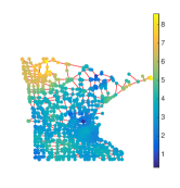
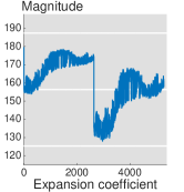
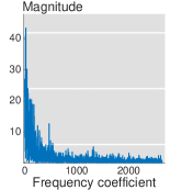
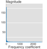
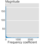
The Minnesota road graph is a standard dataset including 2642 intersections and 3304 roads [40]. we construct a graph by modeling the intersections as nodes and the roads as undirected edges. We collect a dataset recording the wind speeds at those 2642 intersections [41]. The data records the hourly measurement of the wind speed and direction at each intersection. In this paper, we present the data of wind speed on January 1st, 2015. Figure 6(a) shows a snapshot of the wind speeds on the entire Minnesota road. The expansion coefficients obtained by using four representations are shown in Figure 6(b), (c), (d) and (e). The energies of the frequency coefficients of , and mainly concentrate on the low-frequency bands; and are more concentrated; is redundant and the corresponding expansion coefficients are not sparse.
To make a more serious comparison, we evaluate the approximation error by using the normalized mean square error, that is,
| (6) |
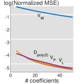
where is the approximation signal and is the original signal. Figure 6(f) shows the approximation errors given by the four representations. The x-axis is the number of coefficients used in approximation, which is in (8) and (III-C1) and the y-axis is the approximation error, where lower means better. We see that and tie ; all of them are much better than . This means that the wind speeds on the Minnesota road graph are well modeled by pairwise Lipschitz smooth, total Lipschitz smooth and local normalized neighboring smooth criteria. The global normalized neighboring smooth criterion is not appropriate for this dataset.
 |
 |
| (a) Temperature. | (b) Coefficients of . |
 |
 |
| (c) Coefficients of . | (d) Coefficients of . |
 |
 |
| (e) Coefficients of . | (f) Approximation err. |
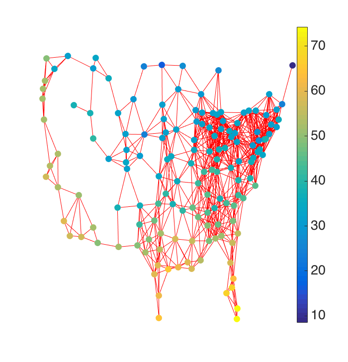
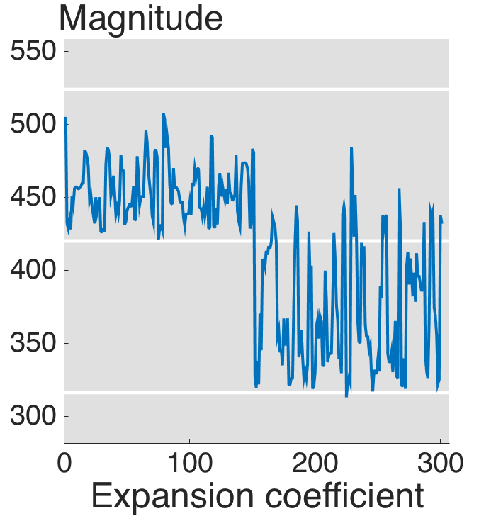
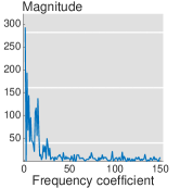
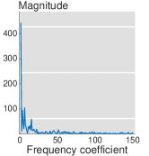
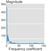
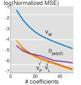
The U.S weather station graph is a network representation of weather stations across the U.S. We assign an edge when two weather stations are within 500 miles. The graph includes nodes and undirected, unweighted edges. Each weather station has days of recordings (one recording per day), for a total of 365 graph signals. As an example, see Figure 7(a). The expansion coefficients obtained by using four representations are shown in Figure 7(b), (c), (d) and (e). Similarly to the wind speed dataset, the energies of the frequency coefficients of , and are mainly concentrated on the low-frequency bands; and are more concentrated; is redundant and the corresponding expansion coefficients are not sparse.
The evaluation metric of the approximation error is also the normalized mean square error. Figure 7(f) shows the approximation errors given by the four representations. The results are averages over 365 graph signals. Again, we see that , and perform similarly; all of them are much better than . This means that the wind speeds on the Minnesota road graph are well modeled by pairwise Lipschitz smooth, total Lipschitz smooth and local normalized neighboring smooth criteria. The global normalized neighboring smooth criterion is not appropriate for this dataset.
The results from two real-world datasets suggest that we should consider using pairwise Lipschitz smooth, total Lipschitz smooth and local normalized neighboring smooth criteria to model real-world smooth graph signals. In terms of the representation dictionary, among , and , is redundant; is not orthonormal. We thus prefer using because it is an orthonormal basis.
IV-C2 Sampling and Recovery
The goal is to recover a smooth graph signal from a few subsamples. A subsample is collected from an individual node each time; that is, we constraint the sampling pattern matrix in (3) be an identity matrix. Previous works show that in this senario, experimentally designed sampling is equivalent to active sampling and is better than uniform sampling asymptotically [42]. Here we compare various sampling strategies based on experimentally designed sampling, which are implemented in a deterministic approach. The random approach sees [6].
Algorithm. We follow the sampling and recovery framework in Section III-C2. Let a smooth graph signal be . For example, , then are the frequency coefficients. In general, we assume that the energy of the expansion coefficient is concentrated in a few known supports, that is, , where and is the known. We aim to recover and further approximate by using . We consider the partial least squares (PLS), , where
where is the noisy version of the graph signal with is noise, and , which is a diagonal matrix with , when the th node is sampled, and 0, otherwise. The recovery error is then
where the first term is bias and the second term is the variance from noise.
We aim to optimize the sampling strategy by minimizing the recovery error and there are six cases to be considered:
-
(a)
minimizing the bias in the worst case; that is,
where is the largest singular value;
-
(b)
minimizing the bias in expectation; that is,
where is the Frobenius norm;
-
(c)
minimizing the variance from noise in the worst case; that is,
-
(d)
minimizing the variance from noise in expectation; that is,
-
(e)
minimizing the recovery error in worst case, that is,
where is related to the signal-to-noise ratio;
-
(f)
minimizing the recovery error in expectation; that is,
where is related to the signal-to-noise ratio.
We call the resulting sampling operator of each setting as an optimal sampling operator with respect to setting (). As shown in the previous work, (c) can be solved by a heuristic greedy search algorithm as shown in [10] and a dual set algorithm as shown in [43]; (d) can be solved by a convex relaxation as shown in [44]. When we deal with a huge graph, can be a huge matrix, solving (a), (b), (e), and (f) can lead to computational issues. When we only want to avoid the interference from a small subset of , we can use a similar heuristic greedy search algorithm to solve (a) and (e) and a similar convex relaxation to solve (b) and (f). Note that the sampling strategies are designed based the recovery strategy of partial least squares; it is not necessary to be optimal in general. Some other recovery strategies are variation minimization algorithms [45, 46, 7, 26]. Comparing to the efficient sampling strategies [26], the optimal sampling operator is more general because it does not require to have any specific property. For example, can contain high-frequency atoms.
Relations to Matrix Approximation. We show that the nodes sampled by the optimal sampling operator are actually the prototype nodes that maximally preserve the connectivity information in the graph structure matrix. In the task of matrix approximation, we aim to find a subset of rows to minimize the reconstruction error. When we specify the matrix to be a graph structure matrix, we solve
where is the subsampling operator in (3) and . [43] shows that
where is the best rank approximation of and is the first columns of the graph Fourier transform matrix of . We see that when , the rows sampled by the optimal sampling operator in (c) minimize the reconstruction error of the graph structure matrix. When sampling nodes, we always lose information, but the optimal sampling operator selects most representative nodes that maximally preserves the connectivity information in the graph structure matrix.
Experiments. The main goal is to compare sampling strategies based on various recovery strategies and datasets.
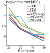
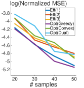
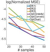
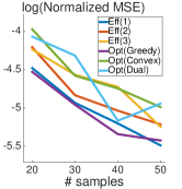
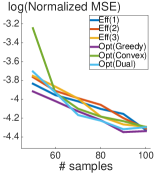
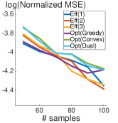
We compare sampling strategies in total. We consider the sampling strategies implementing the optimal sampling operator in three ways: solving the setting (c) by the greedy search algorithm (Opt(G)), solving the setting (c) by the dual set algorithm (Opt(D)) and solving the setting (d) by solving the convex relaxation algorithm (Opt(C)). We also consider the efficient sampling strategies with three parameter settings (Eff(), where is the connection order, varying as ) [26], where the efficient sampling strategies provide fast implementations by taking the advantages of the properties of the graph Laplacian.
We test on recovery strategies in total, including the partial least squares (PLS) (IV-C2), harmonic functions (HF) [45], total variation minimization (TVM) [7] and graph Laplacian based variation minimization with connection order 1 (LVM()) [26]. Note that the proposed optimal sampling operator is based on PLS and the compared efficient sampling strategy is based on LVM.
We test the sampling strategies on two real-world datasets, including the wind speeds on the Minnesota road graph and the temperature measurements on the U.S city graph. As shown in Figures 6 and 7, these signals are smooth on the corresponding graphs, but are not bandlimited.
In Section IV-C1, we conclude that the graph Fourier basis based on graph Laplacian models the graph signals in these two datasets well. We thus specify the first columns of as in (IV-C2), where and is the sample size. The physical meaning of is the bandwidth of a bandlimited space, which means that we design the samples based on a small bandlimited space. We use the same bandwidths in the recovery strategies of the partial least squares and the iterative projection between two convex sets.
 |
 |
| (a) PLS. | (b) HF. |
 |
 |
| (c) TVM. | (d) LVM(1). |
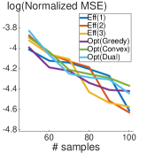
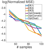
Figures 8 and 9 shows the comparison of sampling strategies based on recovery strategies on the temperature dataset and the wind dataset, respectively. For each figure, the -axis is the number of samples and the -axis is the recovery error, which is evaluated by Normalized MSE (6) in a logarithm scale. For both datasets, three optimal sampling operators are competitive with three efficient sampling strategies under each of recovery strategies. Since efficient sampling strategies need to compute the eigenvectors corresponds to the small eigenvalues, the computation is sometimes unstable when the graph is not well connnected. Within three optimal sampling operators, the greedy search algorithm provides the best performance. As shown in [26], the computational complexity of greedy search algorithm is , where is the number of samples, which is computationally inefficient; however, since we are under the experimentally designed sampling, all the algorithms are designed offline. When the sample size is not too huge, we prefer using a slower, but more accurate sampling strategy. The dual set algorithm also provides competitive performance and the computational complexity of dual set algorithm is , which is more efficient than the greedy search algorithm. Thus, when one needs a small number of samples, we recommend the optimal sampling operator implemented by the greedy search algorithm; when one needs a large number of samples, we recommend the optimal sampling operator implemented by the dual set algorithm.
In [41], the sampling followed with recovery of wind speeds is used to plan routes for autonomous aerial vehicles.
 |
 |
| (a) PLS. | (b) HF. |
 |
 |
| (c) TVM. | (d) LVM(1). |
IV-C3 Case Study: Coauthor Network
We aim to use the proposed approximation and sampling with recovery techniques to large-scale graphs. Here we present some preliminary results.
We collect the publications on three journals, including IEEE Transactions on Signal Processing (TSP), Image Processing (TIP) and Information Theory (TIT). The dataset includes papers on TSP contributed by authors, papers on TIP contributed by authors, papers on TIT contributed by authors. We construct a coauthor network where nodes are unique authors and edges indicate the coauthorship. The edge weight when author and wrote at least one journal together, and , otherwise. The graph includes unique authors and coauthorships. We emphasize unique authors because some of them may publish papers on more than one journals.
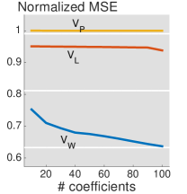
We form a graph signal by count the total number of papers on TSP for each unique author, which describes a distribution of the contribution to the signal processing community. Intuitively, the graph signal is smooth because people in the same community often write papers together. We then check which graph Fourier basis can well represent this smooth graph signal. Since the graph is huge, the full eigendecomposition is computational inefficient and we only compute eigenvectors. For the adjacency matrix, we compute the eigenvectors corresponding the largest eigenvalues; for the graph Laplacian matrix, we compute the eigenvectors corresponding the smallest eigenvalues; for the transition matrix, we compute the eigenvectors corresponding the first eigenvalues with largest magnitudes. Since the graph contains hundreds of disconnected components, the eigenvectors of graph Laplacian matrix do not converge all the time. We use the nonlinear approximation (8) to approximate the graph signal. Figure 10(a) shows the approximation errors based on three graph Fourier bases, , , . We see that the graph Fourier basis based on the adjacency matrix provides much better representation for the graph signal of counting the number of papers in TSP; the first 100 eigenvectors of and capture little information in the graph signal.
When we only have this coauthor network and we aim to have a rough idea of contribution to the signal processing community from each author, it is clear that we do not want to check the publication lists of all the authors. Instead, we can use the sampling and recovery techniques in Section IV-C2 to recover the contribution distribution from a few designed samples. From the aspects of matrix approximation, we aim to select most representative authors and minimize the lost information. Table II list the first 10 authors that we want to query. The first column is sorted based on the total number of papers published in all three transactions in a descending order (degree); the rest of the columns are the designed samples provided by the optimal sampling operator implemented by the greedy search algorithm. We try each of the three graph Fourier bases , and and the samples based on makes more sense. The intuition behind the designed samples is that we want to sample the hub of the large communities in the graph. For example, when two authors wrote many papers together, even both of them have a large number of papers, we only want to sample one from these two. Note that the optimal sampling operator selects most representative authors and it does not rank the importance of each authors.
| Number of publications | |||
|---|---|---|---|
| H. Vincent Poor | H. Vincent Poor | Vishnu Naresh Boddeti | Jang Yi |
| Shlomo Shamai | Aggelos K. Katsaggelos | Kourosh Jafari-Khouzani | Richard B. Wells |
| Dacheng Tao | Truong Q. Nguyen | Y.-S. Park | Akaraphunt Vongkunghae |
| Truong Q. Nguyen | Shuicheng Yan | Gabriel Tsechpenakis | Tsung-Hung Tsai |
| A. Robert Calderbank | Dacheng Tao | Tien C. Hsia | Chuang-Wen You |
| Yonina C. Eldar | Tor Helleseth | James Gonnella | Arvin Wen Tsui |
| Georgios B. Giannakis | Shlomo Shamai | Clifford J. Nolan | Min-Chun Hu |
| Shuicheng Yan | Michael Unser | Ming-Jun Lai | Wen-Huang Cheng |
| Aggelos K. Katsaggelos | Petre Stoica | J. Basak | Heng-Yu Chi |
| Tor Helleseth | Zhi-Quan Luo | Shengyao Chen | Chuan Qin |
V Representations of Piecewise-constant Graph Signals
In classical signal processing, a piecewise-constant signal means a signal that is locally constant in connected regions separated by lower-dimensional boundaries. It is often related to step functions, square waves and Haar wavelets. It is widely used in image processing [19]. Piecewise-constant graph signals have been used in many applications related to graphs without having been explicitly defined; for example, in community detection, community labels form a piecewise-constant graph signal for a social network; in semi-supervised learning, classification labels form a piecewise-constant graph signal for a graph constructed from the dataset. While smooth graph signals emphasize slow transitions, piecewise-constant graph signals emphasize fast transitions (corresponding to boundaries) and localization on the vertex domain (corresponding to signals being nonzeros in a local neighborhood).
V-A Graph Signal Models
We introduce two definitions for piecewise-constant graph signals: one comes from the descriptive approach and the other one comes from the generative approach. We also show their connections.
Let be the graph difference operator (the oriented incidence matrix of ), whose rows correspond to edges [47, 48]. For example, if is a directed edge that connects the th node to the th node (), the elements of the th row of are
where is the weighted adjacency matrix, sgn denotes the sign, which is used to handle the negative edge weights. For a directed graph, and corresponds to two directed edges, representing in two rows in ; for an undirected graph, since , they correspond to a same undirected edge, representing in one row in .
To have more insight on the graph difference operator, we compare it with the graph shift operator. The graph shift operator diffuses each signal coefficient to its neighbors based on the edge weights and is a graph signal representing the shifted version of . The th element of ,
assigns the weighted average of its neighbors’ signal coefficients to the th node. The difference between the original graph signal and the shift version, where is the largest eigenvalue of , is a graph signal measuring the difference of . The term measure the smoothness of a graph signal as shown in Definitions 3 and 4.
The graph difference operator compares the signal coefficients of two nodes connected by each edge and is an edge signal representing the difference of . The th element of ,
assigns the difference between two adjacent signal coefficients to the th edge, where the th edge connects the th node to the th node (). The term also measures the smoothness of . Comparing two measures, emphasizes the neighboring difference, which compares each signal coefficient with the weighted average of its neighbors’ signal coefficients; and emphasizes the pairwise difference, which compares each pair of adjacent signal coefficients. When is an undirected graph, , where is the graph Laplacian matrix, which measures the total Lipschiz smoothness as shown in Definition 2. When the graph is unweighted and all the edge weights are nonnegative, the elements of the th row of are simply
The class of piecewise-constant graph signals is a complement of the class of smooth graph signals, because many real-world graph signals contain outliers, which are hardly captured by smooth graph signals. Smooth graph signals emphasize the slow transition over nodes; and piecewise-constant graph signals emphasize fast transition, localization on the vertex domain: fast transition corresponds to the boundary and localization on the vertex domain corresponds to signals being nonzeros in a local neighbors.
We now define the class of piecewise-constant graph signals.
Definition 9.
A graph signal is piecewise-constant with cuts, when it satisfies
Each element of is the difference between two adjacenct signal coefficient; when , we call the th edge is inconsistent. The class represents signals that contain at most inconsistent edges. For example, when , is the out degree of the th node; when , . From the perspective of graph cuts, we cut inconsistent edges such that a graph is separated into several communities where signal coefficients are the same within each community. Note that Definition 9 includes sparse graph signals. To eliminate sparse graph signals, we can add into the definition.
The piecewise-constant graph signal models in Definition 9 are introduce in a descriptive approach. Following these, we are going to translate the descriptive approach to the generative approach. We construct piecewise-constant graph signals by using local sets, which have been used previously in graph cuts and graph signal reconstruction [49, 8].
Definition 10.
Let be the partition of the node set . We call local sets when they satisfy that the subgraph corresponding to each local set is connected, that is, when is connected for all .
We can represent a local set by using a local-set-based graph signal, , where
For a local-set-based graph signal, we measure its smoothness by the normalized variation
For unweighted graphs, . It measures how hard it is to cut the boundary edges and make an isolated subgraph. We normalize the variation by the size of the local set, which implies that given the same cut cost, a larger local set is more smooth than a smaller local set.
Definition 11.
A graph signal is piecewise-constant based on local sets when
where forms a valid series of local sets. Denote this class by .
When the value of the graph signal on each local set is different, counts the total number of edges connecting nodes between local sets. Definition 11 defines the piecewise-constant graph signal in a generative approach; however, the corresponding representation dictionary has a huge number of atoms, which is impractical to use.
V-B Graph Dictionary
We now discuss representations for piecewise-constant graph signals based on a designed multiresolution local sets. The corresponding representation dictionary has a reasonable size and provides sparse representations for arbitrary piecewise-constant graph signals.
V-B1 Design
We aim to construct a series of local sets in a multiresolution fashion. We first define the multiresolution analysis on graphs.
Definition 12.
A general multiresolution analysis on graphs consists of a sequence of embedded closed subspaces
such that
-
•
upward completeness
-
•
downward completeness
-
•
existence of basis There exists an orthonormal basis for .
Compared with the original multiresolution analysis, the complete space here is instead of because of the discrete nature of a graph; we remove scale invariance and translation invariance because the rigorous definitions of scaling and translation for graphs are still unclear. This is the reason we call it general multiresolution analysis on graphs.
General Construction. The intuition behind the proposed construction is to build the connection between the subspaces and local sets: a bigger subspace corresponds to a finer resolution on the graph vertex domain, or more localized local sets. We initialize to correspond to the th level subspace , that is, . We then partition into two disjoint local sets and , corresponding to the first level subspace , where . We then recursively partition each larger local set into two smaller local sets. For the th level subspace, we have and then, we partition into for all . We call the parent set of and are the children sets of . When , and . At the finest resolution, each local set corresponds to an individual node or an empty set. In other words, we build a binary decomposition tree that partitions a graph structure into multiple local sets. The th level of the decomposition tree corresponds to the th level subspace. The depth of the decomposition depends on how local sets are partitioned; ranges from to , where corresponds to partitioning one node at a time and corresponds to an even partition at each level.
It is clear that the proposed construction of local sets satisfies three requirements in Definition 12. The initial subspace has the coast resolution. Through partitioning, local sets zoom into increasingly finer resolutions in the graph vertex domain. The subspace with finest resolution zoom into each individual node and covers the entire . Classical scale invariance requires that when , then , which is ill-posed in the graph domain because graphs are finite and discrete; the classical translation invariance requires that when , then , which is again ill-posed, this time because graphs are irregular. The essence of scaling and translation invariance, however, is to use the same function and its scales and translates to span different subspaces, which is what the proposed construction promotes. The scaling function is ; the hierarchy of partition is similar to the scaling and translation, that is, when , then , and when then .
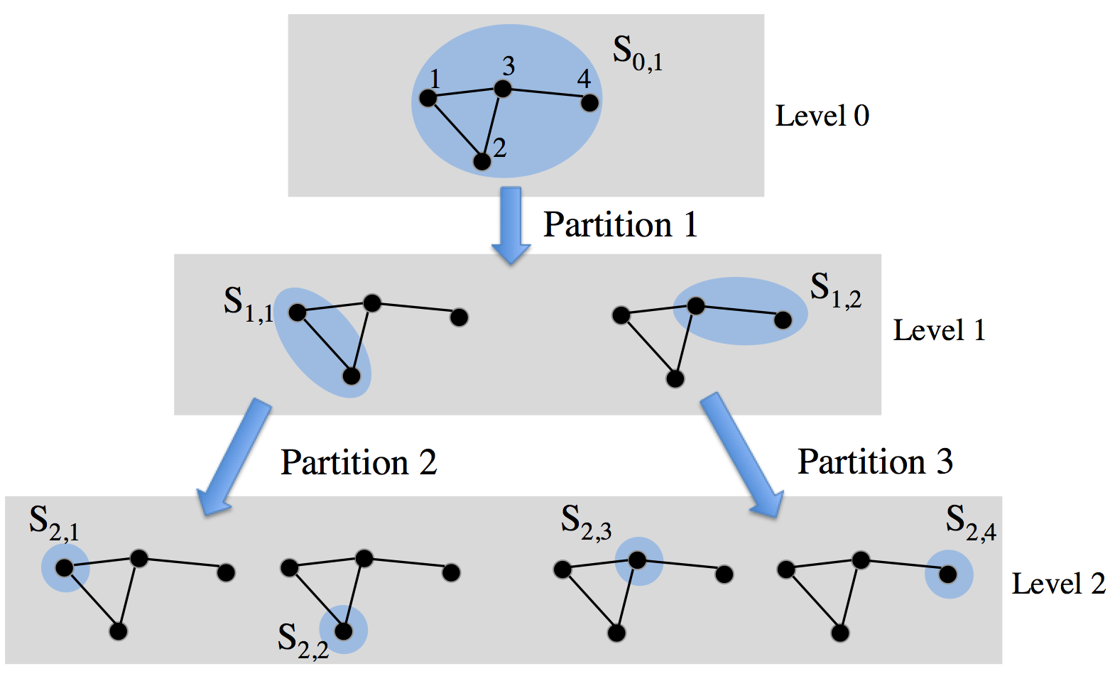
To summarize the construction, we build a local set decomposition tree by recursively partitioning a local set into two disjoint local sets until that all the local sets are individual nodes. We now show a toy example in Figure 11. In Partition 1, we partition the entire node set into two disjoint local sets . Thus, . Similarly, in Partition 2, we partition into two disjoint connected sets ; in Partition 3, we partition into . Thus, .
Graph Partition Algorithm. The graph partition is the key step to construct the local sets. From the perspective of promoting smoothness of graph signals, we partition a local set into two disjoint local set by solving the following optimization problem
Ideally, we aim to solve V-B1 to obtain two children local sets, however, it is nonconvex and hard to solve. Instead, we consider three relaxed methods to partition a graph.
The first one is based on spectral clustering [49]. We first obtain the graph Laplacian matrix of a local set and compute the eigenvector corresponding to the second smallest eigenvalue of the graph Laplacian matrix. We then set the median number of the eigenvector as the threshold; we put the nodes whose corresponding values in the eigenvector are no smaller than the threshold into a children local set and put the nodes whose corresponding values in the eigenvector are smaller than the threshold into the other children local set. This method approximately solves V-B1 by ignoring the second constraint; it guarantees that two children local sets have the same number of nodes, but does not guarantee that they have the same number of nodes are connected.
The second one is based on spanning tree. To partition a local set, we first obtain the maximum spanning tree of the subgraph and then find a balance node in the spanning tree. The balance node partition the spanning tree into two subtrees with the closet number of nodes [50]. We remove the balance node from the spanning tree, the resulting largest connected component form a children local set and the other nodes including the balance node forms the other children local set. This method approximately solves V-B1 by approximating a subgraph by the corresponding maximum spanning tree; it guarantee that two children local sets are connected, but does not guarantees that they have the same number of nodes. When the original sbugraph is highly connected, the spanning tree loses some connection information and the shape of the local set may not capture the community in the subgraph.
The third one is based on the 2-means clustering. We first randomly select 2 nodes as the community center and assign every other node to its nearest community center based on the geodesic distance. We then recompute the community center for each community by minimizing the summation of the geodesic distances to all the other nodes in the community and assign node to its nearest community center again. We keep doing this until the community centres converge after a few iterations. This method is inspired from the classical -means clustering; it also guarantees that two children local sets are connected, but does not guarantees that they have the same number of nodes.
In general, the proposed construction of local sets does not restrict to any particular graph partition algorithm; depending on the applications, the partition step can also be implemented by many other existing graph partition algorithms.
Dictionary Representations. We collect local sets by level in ascending order in a dictionary, with atoms corresponding to each local set, that is, . We call it the local-set-based piecewise-constant dictionary. After removing empty sets, the dictionary has atoms, that is, ; each atom is a piecewise-constant graph signal with various sizes and localizing various parts of a graph.
Wavelet Basis. We construct a wavelet basis based on the local-set-based piecewise-constant dictionary. We combine two local sets partitioned from the same parent local set to form a basis vector. Let the local sets have the same parent local set , the basis vector combing these two local sets is
To represent in a matrix form, the wavelet basis is
where the downsampling matrix
with is the th column of , and
The downsampling matrix combines two consecutive column vectors in to form one column vector in and the function reweights the column vectors in to ensure that each column vector in has norm 1 and sums to 0.
Another explanation is that when we recursively partition a node set into two local sets, each partition generates a wavelet basis vector. We still use Figure 11 as an example. In Partition 1, we partition the entire node set into and generate a basis vector
in Partition 2, we partition into two disjoint connected sets and generate a basis vector
in Partition 3, we partition into and generate a basis vector
We summarize the construction of the local-set-based wavelet basis in Algorithm 1.
| Input | graph | |
| Output | wavelet basis | |
| Function | ||
| initialize a stack of node sets and a set of vectors | ||
| push into | ||
| add into | ||
| while the cardinality of the largest element of is bigger than | ||
| pop up one element from as | ||
| partition into two disjoint connected sets | ||
| push into | ||
| add into | ||
| end | ||
| return |
V-B2 Properties
We now analyze some properties of the proposed construction of the local sets and wavelet basis. The main results are
-
•
the local-set-based dictionary provides a multiresolution representation;
-
•
there exists a tradeoff between smoothness and fine resolution in partitioning the local sets;
-
•
the local-set-based wavelet basis is an orthonormal basis;
-
•
the local-set-based wavelet basis promotes sparsity for piecewise-constant graph signals.
Theorem 6.
The proposed construction of local sets satisfies the multiresolution analysis on graphs.
We have shown this in the previous section. We list here for completeness. In the original multiresolution analysis, more localization in the time domain leads to more high-frequency components. Here we show a similar result.
Theorem 7.
A series of local sets with a finer resolution is less smooth, that is, for all ,
Proof.
We first show that the sum of variations of two children local sets is larger than the variation of the parent local set.
where follows from that the cardinality of the the parent local set is larger than either of its children local sets and follows from that we need to cut a boundary to partition two children local sets. Since every local set in the th level has two children local sets in the th level and every local set in the th level has a parent local set in the th local, we sum them together and obtain Theorem 7. ∎
Theorem 7 shows that by zooming in the graph vertex domain, the partitioned local sets get less smooth; in other words, we have to tradeoff the smoothness to obtain a finer resolution.
We next show that the local-set-based wavelet basis is a valid orthonormal basis.
Theorem 8.
The local-set-based wavelet basis constructs an orthonormal basis.
Proof.
First, we show each vector has norm one.
where follows from that . Second, we show each vector is orthogonal to the other vectors. We have
Thus, each vector is orthogonal to the first vector, . Each other individual vector is generated from two node sets. Let generate and generate . Due to the construction, there are only two conditions, two node sets of one vector belongs to one node set of the other vector, and all four node sets do not share element with each other. For the first case, without losing generality, let , we have
For the second case, the inner product between and is zero because their supports do not match. Third, we show that spans . Since we recursively partition the node set until the cardinalities of all the node sets are smaller than 2, there are vectors in . ∎
We show that the local-set-based wavelet basis is a good representation for piecewise-constant graph signals through promoting the sparsity.
Theorem 9.
Proof.
When an edge , where Supp denotes the indices of nonzero elements, we call that the edge is activated by the vector . Since each edge is activated at most once in each decomposition level, so each edge is activated by at most basis elements. Let activations() be the number of basis elements in that activates .
∎
The maximum level of the decomposition is determined by the choice of graph partition algorithm. Theorem 1 shows that what it matters is the cardinality of each local set, instead of the shape of each local set. To achieve the best sparse representation, we should partition each local set as evenly as possible. Note that when the partition is perfectly even, the resulting wavelet basis is the same with the classical Haar wavelet basis.
Corollary 1.
For all , we have , where is the maximum level of the decomposition and
Since is obtained from , the worst case is to represent by using .
Corollary 2.
Let the local-set-based wavelet basis evenly partition the node set each time. We have
We see that the local-set-based piecewise-constant wavelet basis provides a sparse representation for the piecewise-constant graph signals. We conjecture the proposed construction is the optimal orthonormal basis to promote the sparsity for piecewise-constant graph signals.
Conjecture 1.
Let be the local-set-based wavelet basis with the even partition. Then,
In general, the graph difference operator provides more sparse representation than the local-set-based wavelet basis, however, the graph difference operator is not necessarily a one-to-one mapping and is bad at reconstruction; the graph difference operator only focuses on the pairwise relationship. On the other hand, the local-set-based wavelet basis is good at reconstruction and provides multiresolution view in the graph vertex domain.
The even partition minimizes the worst case; it does not necessarily mean that the even partition is good for all the applications. For example, a graph has two communities, a huge one and a tiny one, which hints that a piecewise-constant graph signal sits on a part of either of two communities. In this case, we cut a few edges to partition two communities and assign a local set for each of them, instead of partitioning the huge community to make sure that two local sets have a same cardinality.
V-C Graph Signal Processing Tasks
V-C1 Approximation
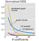
Approximation is a standard task to evaluate a representation and it is similar to compression. The goal is to use a few expansion coefficients to approximate a graph signal. We compare the graph Fourier transform [1], the windowed graph Fourier transform [20], the local-set-based wavelet basis and dictionary. The graph Fourier transform is the eigenvector matrix of the graph shift and the windowed graph Fourier transform provides vertex-frequency analysis on graphs. For the local-set-based piecewise-constant wavelet basis and dictionary, we also consider three graph partition algorithms, including spectral clustering, spanning tree and 2-means.
Algorithm. Since the graph Fourier transform and the local-set-based wavelet bases are orthonormal bases, we consider nonlinear approximation for the graph Fourier bases, that is, after expanding in with a representation, we should choose the largest-magnitude expansion coefficients so as to minimize the approximation error. Let and be a pair of biorthonormal basis and be a signal. Here the graph Fourier transform matrix and the graph Fourier basis . The nonlinear approximation to is
| (8) |
where is the index set of the largest-magnitude expansion coefficients. When a basis promotes sparsity for , only a few expansion coefficients are needed to obtain a small approximation error. Note that (8) is a special case of (III-C1) when the distance metric is the norm and is an orthonormal basis.
Since the the windowed graph dictionary and the local-set-based piecewise-constant dictionaries are redundant, we solve the following sparse coding problem,
where is a redundant dictionary and is a sparse code. The idea is to use a linear combination of a few atoms from to approximate the original signal. When is an orthonormal basis, the closed-form solution is exactly (8). We solve (III-C1) by using the orthogonal matching pursuit, which is a greedy algorithm [39]. Note that (V-C1) is a special case of (III-C1) when the distance metric is the norm.
Experiments. We test the four representations on two datasets, including the Minnesota road graph [40] and the U.S city graph [7].
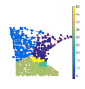
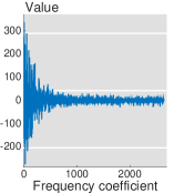
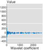
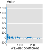
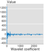
For the Minnesota road graph, we simulate a piecewise-constant graph signal by randomly picking 5 nodes as community centers and assigning each other node to its nearest community center based on the geodesic distance. We assign a random integer to each community. The simulated graph signal is shown in Figure 12. The signal contains piecewise constants and inconsistent edges. The frequency coefficients and the wavelet coefficients obtained by using three graph partition algorithms are shown in Figure 12(b), (c), (d) and (e). The sparsities of the wavelet coefficients for spectral clustering, spanning tree, and 2-means are , , and , respectively; the proposed wavelet bases provide much better sparse representations than the graph Fourier transform.
The evaluation metric of the approximation error is the normalized mean square error, that is,
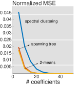
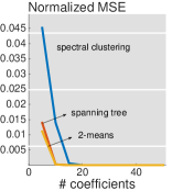
where is the approximation signal and is the original signal. Figure 12(f) shows the approximation errors given by the four representations. The x-axis is the number of coefficients used in approximation, which is in (8) and (III-C1) and the y-axis is the approximation error, where lower means better. We see that the local-set-based wavelet with spectral clustering and local-set-based dictionary with spectral clustering provides much better performances and the windowed graph Fourier transform catches up with graph Fourier transform around expansion coefficients. Figure 12(g) and (h) compares the local-set-based wavelets and dictionaries with three different partition algorithms, respectively. We see that the spanning tree and 2-means have similar performances, which are better than spectral clustering. This is consistent with the sparsities of the wavelet coefficients, where the wavelet coefficients of spanning tree and 2-means are more sparse than those of spectral clustering.
 |
 |
| (a) Signal. | (b) Frequency coefficients. |
 |
 |
| (c) Wavelet coefficients | (d) Wavelet coefficients |
| from spectral clustering. | from spanning tree. |
 |
 |
| (e) Wavelet coefficients | (f) Error comparison. |
| from 2-means. | |
 |
 |
| (g) Error (Wavelet) | (h) Error (Dictionary). |
The U.S city graph is a network representation of weather stations across the U.S. We assign an edge when two weather stations are within 500 miles. The graph includes nodes and undirected, unweighted edges. Based on the geographical area, we partition the nodes into four communities, including the north area (N), the middle area (M), the south area (S), and the west area (W). The corresponding piecewise-constant graph signal is
| (10) |
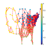
The graph signal is shown in Figure 13(a), where dark blue indicates the north area, the light indicates the middle area, the dark yellow indicates the south area and the light yellow indicates the west area. The signal contains piecewise constants and inconsistent edges.
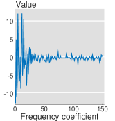
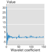
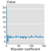
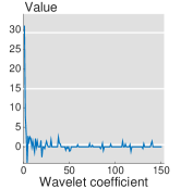
The frequency coefficients and the wavelet coefficients obtained by using three graph partition algorithms are shown in Figure 13(b), (c), (d) and (e). The sparsities of the wavelet coefficients for spectral clustering, spanning tree, and 2-means are , , and , respectively; the proposed wavelet bases provide much better sparse representations than the graph Fourier transform.
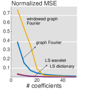
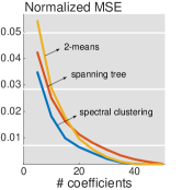
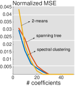
The evaluation metric of the approximation error is also the normalized mean square error. Figure 13(f) shows the approximation errors given by the four representations. Similarly to Figure 13(d), the local-set-based wavelet with spectral clustering and local-set-based dictionary with spectral clustering provides much better performances and the windowed graph Fourier transform catches up with graph Fourier transform around expansion coefficients. Figure 13(g) and (h) compares the local-set-based wavelets and dictionaries with three different graph partition algorithms, respectively. We see that the spectral clustering provides the best performance.
 |
 |
| (a) Signal. | (b) Frequency coefficients. |
 |
 |
| (c) Wavelet coefficients | (d) Wavelet coefficients |
| from spectral clustering. | from spanning tree. |
 |
 |
| (e) Wavelet coefficients | (f) Error comparison. |
| from 2-means. | |
 |
 |
| (g) Error (wavelet). | (h) Error (dictionary). |
To summarize the task of approximation, the proposed local set based representations provide a reliable approximation to a piecewise-constant graph signal because of the sparsity promotion.
V-C2 Sampling and Recovery
The goal of sampling and recovery is to collect a few samples from a graph signal, and then to recover the original graph signal from those samples either exactly or approximately. Similar procedures are widely used in many applications, such as semi-supervised learning and active learning .
Algorithm. We consider the following recovery algorithm based on the multiresolution local sets. Let be the number of samples. We use the multiresolution decomposition of the local sets as shown in Section V-B1. Instead of obtaining a full decomposition tree, we partition the local sets until we obtain leaf local sets. Those local sets may not be in the same decomposition level , but the union of them still cover the entire space. For the local sets in the same level of the decomposition tree, we first partition the one that has the largest number of nodes. For each leaf local set, we choose a center that has the minimum summation of the geodesic distances to all the other nodes in the leaf local set. We use those centers for the leaf local sets as the sampled set. Let be a piecewise-constant graph signal, be the designed sampled set, with each sampled node be the center of the th leaf local set . The recovered graph signal is
We obtain a simple upper bound for the recovery error of this algorithm.
Theorem 10.
Let the original graph signal . The recovery error is bounded as
where is the indicator function.
Proof.
The error happens only when there exists at least one inconsistent edge in a community. Since there are inconsistent edges, we make errors in at most communities. The worst case is that each error is made in the one of the largest communities. ∎
Theorem 10 shows that the size of the largest community influences the recovery error. When we use the even partition, the size of the largest local set is minimized, which minimizes the upper bound. Similar to Theorem 1, Theorem 10 also shows the importance of the even partition again. This algorithm studies the graph structure before taking samples, which belongs to the experimentally designed sampling. In the classical regression for piecewise-constant functions, it is known that experimentally designed sampling has the same performance with random sampling asymptotically [51]. When we restrict the problem setting to sample only a few nodes from a finite graph, however, random sampling can lead to the uneven partition where some communities are much larger than the others. As a deterministic approach, the experimentally designed sampling minimizes the error bound and is better than random sampling when the sample size is small.
We also consider two other recovery algorithms, including trend filtering on graphs and harmonic functions. For trend filtering on graphs, we consider
where is the sampling node set obtained by random sampling. We want to push the recovered graph signal to be close to the original one at the sampled nodes and to be piecewise constant. For harmonic functions, we consider
where and is the graph Laplacian matrix. Harmonic functions are proposed to recover a smooth graph signal which can be treated as an approximation of a piecewise-constant graph signal. When we obtain the solution, we assign each coefficient to its closest constant in .
Experiments. We test the four representations on two datasets, including the Minnesota road graph [40] and the U.S city graph [7].
For the Minnesota road graph, we simulate a piecewise-constant graph signal by randomly picking 5 nodes as community centers and assigning each other node a community label based on the geodesic distance. We assign a random integer to each community. We still use the simulated graph signal in Figure 12(a).
The evaluation metric of the recovery error is the percentage of mislabel, that is,
where is the recovered signal and is the ground-truth signal. Figure 14(a) shows the recovery errors given by three algorithms. The x-axis is the ratio between the number of samples and the total number of nodes and the y-axis is the recovery error, where lower means better. Since harmonic functions and trend filtering are based on random sampling, the results are averaged over 50 runs. SC indicates spectral clustering, ST indicates spanning tree and 2M indicates 2-means. We see that the local-set-based recovery algorithms are better than harmonic functions and trend filtering, especially when the sample ratio is small.
For the U.S city graph, we use the same piecewise-constant graph signal (10) as the ground truth. The evaluation metric of the recovery error is the percentage of mislabel. Figure 14(b) shows the recovery errors given by three recovery strategies with two different sampling strategies. Similarly to the recovery of the Minnesota road graph, we see that the local-set-based recovery algorithms are better than harmonic functions and trend filtering, especially when the sample ratio is small.
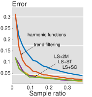 |
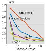 |
| (a) Minnesota road graph. | (b) U.S. city graph |
To summarize the task of sampling and recovery, the proposed center-assign algorithm is simple and useful in the recovery. The experimentally designed sampling based on local sets tries to minimizes the upper bound in Theorem 10 and make each local set have similar sizes. It provides a deterministic approach to choose sampled nodes; it works better than random sampling when the sample ratio is small and have a similar performance with random sampling asymptotically.
V-C3 Case Study: Epidemics Process
Epidemics process has been modeled as the diffusion process of ideas/opinions/beliefs/innovations over a finite-sized, static, connected social network [52]. In the terminology of epidemics, if the state of each node is either susceptible or infected, it is usually model by the susceptible-infected-susceptible (SIS) model. Nodes that are infected have a certain rate () to recover and return to be susceptible; nodes that are susceptible can be contagious if infected by its neighboring infected nodes under certain rate ().
Here we adopt the SIS model on network, which takes the network structure into account and help us estimate the macroscopic behavior of an epidemic outbreak [53]. In SIS model on network, is the infection rate quantify the probability per unit time that the infection will be transmitted from an infective individual to a susceptible one, is the recovery (or healing) probability per unit time that an infective individual recovers and becomes susceptible again. To be more accurate, the infection rate studied here is a part of endogenous infection rate, which has the form of , where is the number of infected neighbors of the susceptible node [52, 54]. Since dependents on the structure of the network, is referred as topology dependent infection rate, and since recovery is a spontaneous action and the recovery probability is identical for all the infective nodes, is considered to be network topology independent [52].
We consider a task to estimate the disease incidence, or the percentage of the infected nodes at each time. A simple method is that, in each time, we randomly sample some nodes, query their states, and calculate the percentage of the infected nodes. This method provides an unbiased estimator to estimate the disease incidence. However, this method has two shortcomings: first, it loses information on graphs and cannot tell which nodes are infected; second, since it is a random approach, it needs a huge number of samples to ensure a reliable estimation.
We can model the states of nodes as a graph signal where represents infective and represents susceptible. When the topology dependent infection rate is high and the healing probability is low, the infection spreads locally; that is, nodes in a same community get infected in a same time and the corresponding graph signal is piecewise constant. We can use the sampling and recovery algorithm in Section V-C2 and then calculate the percentage of the infected nodes in the recovered graph signal. In this way, we can visualize the graph and tell which nodes may be infected because we recover the states of all the nodes; we also avoid the randomness effect because the algorithm is based on the experimentally designed sampling.
We simulate an epidemics process over the Minnesota road graph by using the SIS model. We set be , and be . In the first day, we randomly select three nodes to be infected and diffuses it for days. Figure 15 shows the states of nodes in the th day and the th day. We see that three small communities are infected in the th day; these communities are growing bigger in the th day. Since the healing probability is nonzero, a few susceptible nodes still exist within the communities.
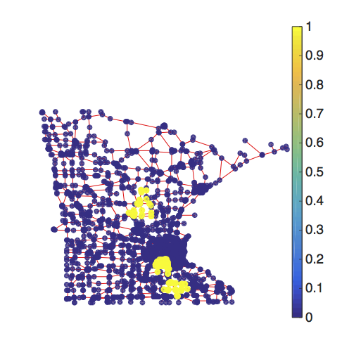 |
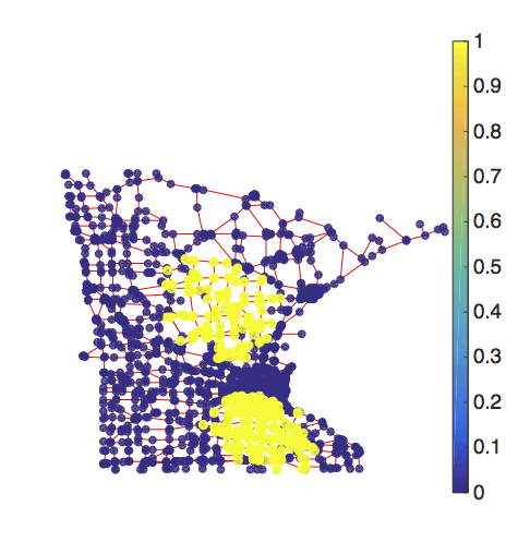 |
| (a) th day. | (b) th day. |
We compare the results of two algorithms: one is based on random sampling following with calculating the percentage of infection within the sampled nodes; the other one is based on the local-set-based recovery algorithm following with calculating the percentage of infection within the recovered graph signal. The evaluation metric is the frequency that the result of the local-set-based recovery algorithm is closer to the groundtruth, that is,
where is the ground truth of the percentage of infection, is the estimation of the random algorithm in the th trials, is the estimation of the local-set-based recovery algorithm, and is the total number of random trials; we choose here. The success rate measures the frequency when the local-set-based recovery algorithm has a better performance. When the success rate is bigger than , the local-set-based recovery algorithm is better; When the success rate is smaller than , the random algorithm is better. Figure 16 shows the success rates given by the local-set-based recovery with three different graph partition algorithms. In each figure, the x-axis is the day ( days in total); the y-axis is the success rate; the darker region means that local-set-based recovery algorithm fails and the lighter region means that local-set-based recovery algorithm successes; and the number shows the percentage of success or fail within 50 days. We see that given 100 samples, the local-set-based recovery algorithms are slightly worse than the random algorithm; given 1000 samples, the local-set-based recovery algorithms are slightly better than the random algorithm.
 |
 |
| (a) Spectral clustering | (b) Spectral clustering |
| with samples. | with samples. |
 |
 |
| (c) Spanning tree | (d) Spanning tree |
| with samples. | with samples. |
 |
 |
| (e) 2-means | (f) 2-means |
| with samples. | with samples. |
In Figure 17, we show the recovered states by the local-set-based recovery algorithm with 2-means partition on the th day. When having a few samples, the local-set-based recovery algorithms can recover the states in general, but cannot zoom into details and provide accurate estimations; when taking more samples, the local-set-based recovery algorithms recover the states better and provide better estimations. We see that the local-set-based recovery algorithm with 2-means partition provides both good estimation and good visualization.
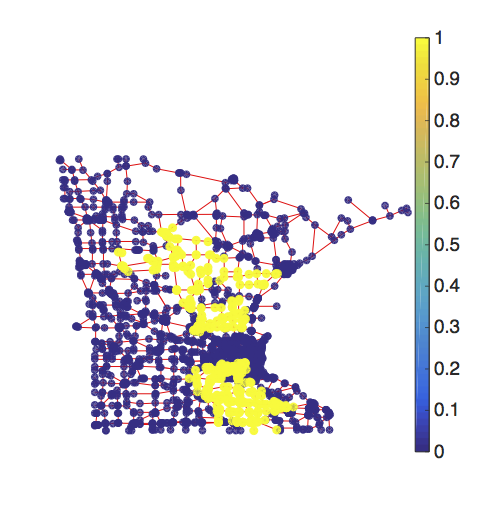 |
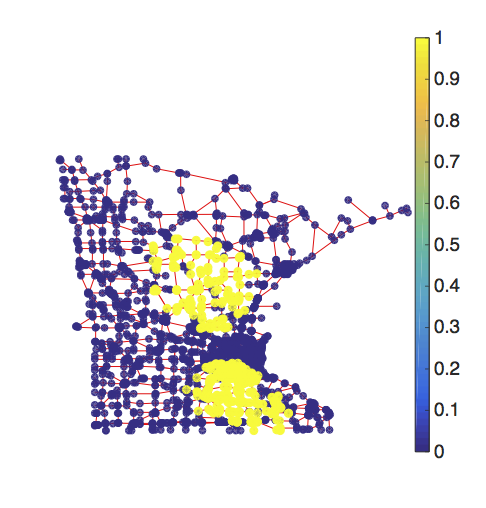 |
| (e) 2-means | (f) 2-means |
| with samples. | wiith samples. |
VI Representations of Piecewise-smooth Graph Signals
To be able to deal with as wide a class of real-world graphs signals as possible, we combine smooth and piecewise-constant graph signals into piecewise-smooth graph signals.
VI-A Graph Signal Models
Based on smooth graph signal models, we have two types of piecewise-smooth signal models, including the piecewise-polynomial class and the piecewise-bandlimited class.
Definition 13.
A graph signal is piecewise-polynomial with pieces and degree when
where is a th order polynomial signal on the subgraph with Denote this class by .
is the polynomial class with degree , from Definition 5, and is the piecewise-constant class with pieces, from Definition 11. The degrees of freedom for a local set at the polynomial degree is the number of origins, that is,
Definition 14.
A graph signal is piecewise-bandlimited with pieces and bandwidth when
where is a bandlimited signal on the subgraph with , and is a graph Fourier basis of . Denote this class by .
We use zero padding to ensure for each . Still, can be the eigenvector matrix of the adjacency matrix, graph Laplacian matrix or the transition matrix.
VI-B Graph Dictionary
The representations of piecewise-smooth graph signals is based on the local-set piecewise-constant dictionary. To represent piecewise-smooth graph signals, we use multiple atoms for each local set. We take the piecewise-polynomial signals as an example. For each local set,
where , when ; and 0, otherwise. The number of atoms in is . We collect the sub-dictionaries for all the multiresolution local sets to form the local-set-based piecewise-smooth dictionary, that is, . The number of atoms in is , where is the maximum degree of polynomial, is the size of the graph and is the maximum level of the decomposition. When we use even partitioning, the total number of atoms is .
Similarly, to model piecewise-bandlimited signals, we replace by the graph Fourier basis of each subgraph . The total number of atoms of the corresponding is then . For piecewise-smooth signals, we cannot use the sparse coding to do exact approximation. To minimize the approximation error, both the sizes and the shapes of the local sets matter for piecewise-smooth graph signals.
VI-B1 Properties
Theorem 11.
For all , where is the graph Fourier basis of the graph Laplacian matrix , we have , where is the maximum level of the decomposition, is a piecewise-constant signal that corresponds the same local sets with and
where is a constant determined by graph partitioning.
Proof.
The main idea is that we approximate a bandlimited signal in the original graph by using bandlimited signals in subgraphs. Based on the eigenvectors of graph Laplacian matrix, we define the bandlimited space, where each signal can be represented as where is the submatrix of containing the first columns in . We can show that this bandlimited space is a subspace of the total pairwise smooth space .
where is the graph Laplacian matrix of the subgraph and stores the residual edges, which are cut in the graph partition algorithm.
Thus, is a subset of ; that is, any total pairwise smooth graph signal in the whole graph can be precisely represented by total pairwise smooth graph signals in the subgraphs.
In each local set, when we use the bandlimited space to approximate the space , the maximum error we suffer from is , which is solved by the following optimization problem,
In other words, in each local set, the maximum error to represent is . Since all the local sets share the variation budget of together, the maximum error we suffer from is .
We further use the local-set piecewise-smooth dictionary to detect piecewise-smooth signals from random noises.
Theorem 12.
We consider statistically testing the null and alternative hypothesis,
We solve the following optimization problem
by using the matching pursuit algorithm. We reject the null if . Set . If
where . Then under , , and under , .
Proof.
Under the null, we have with probability at least . We set to control the type 1 error.
For the alternative, with probability . In Theorem 11, we see that it is feasible to have with . We then have
where is the support of zero elements in . Then, we force the lower bound of to control the type 2 error. ∎
VI-C Graph Signal Processing Tasks
VI-C1 Approximation
Good approximation for piecewise-smooth graph signals are potentially useful in many applications, such as visualization, denoising, active sampling [51, 6] and semi-supervised learning [55]. Similarly to Section V-C1, we compare the windowed graph Fourier transform [20] with the local-set-based dictionaries. We use the balance cut of the spanning tree to obtain the local sets [50]. The approximation is implemented by solving the sparse coding problem (V-C1).
Experiments. We still test the representations on two datasets, the Minnesota road graph [40] and the U.S city graph [7]. On the Minnesota road graph, we simulate piecewise-constant graph signals as follows: we random choose three nodes as cluster centers and assign all other nodes to their nearest cluster centers based on the geodesic distance. We assign a random integer to each cluster. We further obtain piecewise-polynomial graph signals by element-wise multiplying a polynomial function, , where is a reference node that assigns randomly. As an example, see Figure 18(a).
On the U.S city graph, we use the real temperature measurements. The graph includes 150 weather stations and each weather station has days of recordings (one recording per day), for a total of 365 graph signals. As an example, see Figure 18(b).
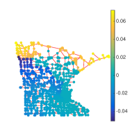 |
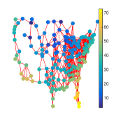 |
| (a) Minnesota. | (b) U.S weather station. |
The approximation error is measured by the normalized mean square error. Figure 19 shows the averaged approximation errors. LSPC denotes local-set-based piecewise-constant dictionary and LSPS denotes local-set-based piecewise-smooth dictionary. For the windowed graph Fourier transform, we use filters; for LSPS, three piecewise-smooth models provide tight performances; here we show the results of the piecewise-polynomial smooth model with degree . We see that the local-set-based dictionaries perform better than the windowed graph Fourier transform; local-set-based piecewise-smooth dictionary is slightly better than local-set-based piecewise-constant dictionary; even though the windowed graph Fourier transform is solid in theory, provides highly redundant representations and is useful for visualization, it does not well approximate complex graph signals.
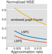 |
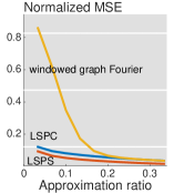 |
| (a) Minnesota. | (b) U.S weather station. |
VI-C2 Sampling and Recovery
The sampling and recovery techniques of piecewise-smooth graph signals are similar to those of smooth graph signals. The basic idea is to assume the energy of a graph signal concentrates on a few expansion coefficients. For smooth graph signals, it is clear that the energy concentrates on the low-pass frequency band; however, for piecewise-smooth graph signals, we do not have any prior knowledge. We leave the blind recovery as the future work. Some related works about the blind recovery are discussed in [56, 57].
VI-D Case Study: Environmental Change Detection
This case study is motivated to providing an intuitive and reliable approach to detect environmental change using sparse coding. The detected change has many potential applications, such as offering suggestion to the authorities, or monitoring the variation trend in a local or global view. Besides, most environmental data is collected by sensors, detecting anomaly records can give prior knowledge on the status of sensors and functioned as a pre-processing procedure for subsequent sensor data analysis.
We study the daily distribution of \ceSO2 during in mainland U.S., the underlying graph is composed by operating sensors, which record the daily average at various locations. Since the adjacent sensors have similar records, we model the daily graph signal as a piecewise smooth signal, and build local-set-based piecewise-smooth dictionary (), introduced in VI-B to represent it. In the experiment is considered as a piecewise polynomial dictionary.
In this case study, our task is that for arbitrary successive two days, we use the proposed dictionary to detect the areas that whose recorded data changed the most saliently between the two days. The intuition behind this is that the difference of the recorded \ceSO2 will have bigger magnitude in the targeted areas compared with their neighborhood, and the proposed multi-resolution dictionary can zoom into that certain areas so to detect them. Mathematically, the areas are encoded in the activated atoms corresponding to the top sparse coding coefficient in terms of magnitude. We use the matching pursuit to get the sparse coding of with respect to the built dictionary.
In Figure 20, we aim to illustrate the benefits of the proposed graph dictionary on detecting the very area whose recorded data changed the most from to . Figure 20 (a) (b) show the snapshot of \ceSO2 distributed on and , (c) illustrates the snapshot of data records difference between these two days. (d), (e) show the detected area by the activated atom corresponding to the top and sparse coding coefficient, and they contain and nodes, respectively. As comparison, in (f) we rank the records difference in terms of magnitude and highlight the top nodes. Since (f) is generated without taking the graph structure into account, the highlighted nodes spread out; while the graph dictionary has the graph information built in, the highlighted nodes in (d) and (e) cluster into group, and give us a better geographical knowledge on which part of U.S. having \ceSO2 distribution changes the most during these two days. In this experiment, is built by 2-means graph partition algorithm, other graph partition algorithms, spectral clustering and spanning tree, can also build graph dictionary that are good at detect records data change, and can provide better geographical knowledge than just simply rank the difference coefficient.
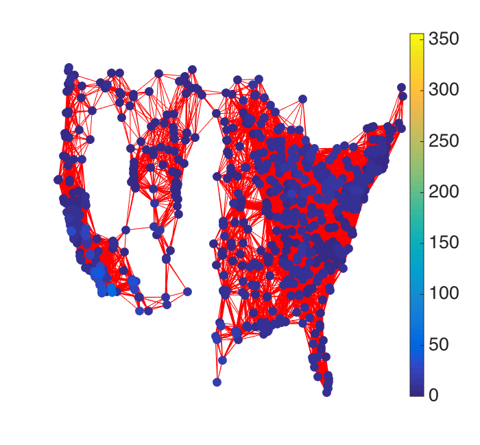 |
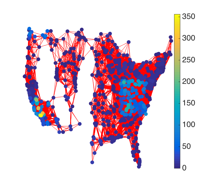 |
| (a) Snapshot of \cePM_2.5 | (b) Snapshot of corrupted |
| on . | \cePM_2.5 on . |
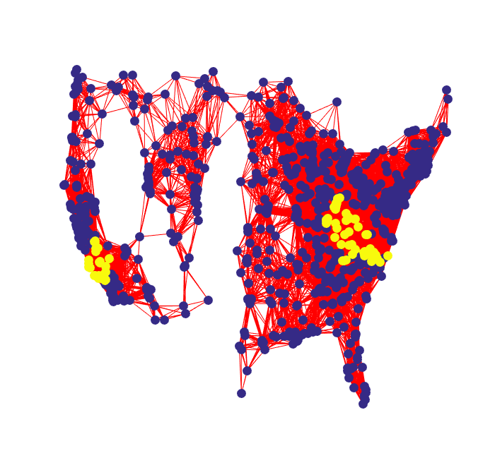 |
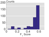 |
| (c) Detected area by atoms | (d) Histogram of Score |
| corresponding to top | of detected areas |
| using spectral clustering. | using spectral clustering. |
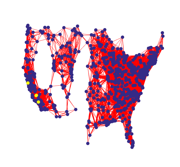 |
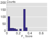 |
| (e) Detected area by atoms | (f) Histogram of Score |
| corresponding to top | of detected areas |
| using MST. | using MST. |
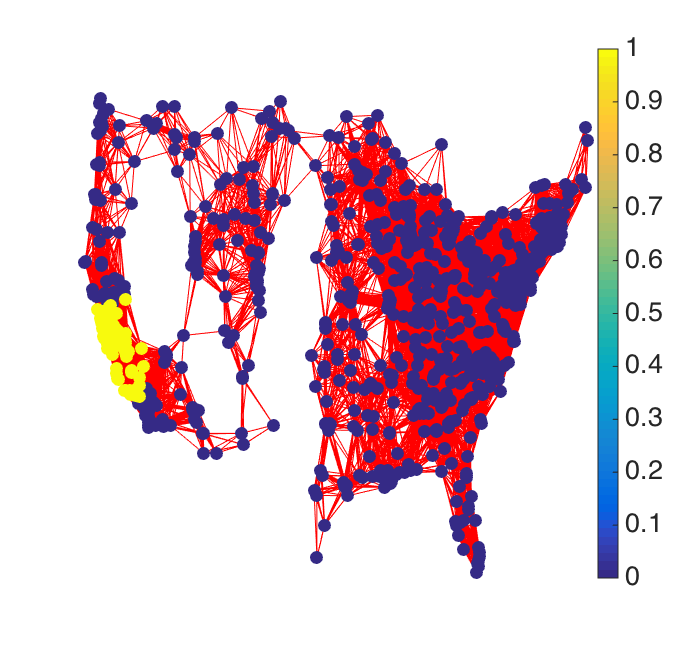 |
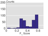 |
| (g) Detected areas by atoms | (h) Histogram of Score |
| corresponding to top . | of detected areas |
| using 2-means. | using 2-means. |
VII Conclusions
Graph signal representation has been considered in many previous literature [30, 2, 29, 14]. There are mainly two approaches to design a representation for graph signals: one is based on the graph Fourier domain and the other one is based on the graph vertex domain.
The representations based on the graph Fourier domain are based on the spectral properties of the graph. The most fundamental representation based on the graph Fourier domain is the graph Fourier transform, which is the eigenvectors of a matrix that represents a graph structure [29, 1]. Based on the graph Fourier transform, people propose various versions of multiresolution transforms on graphs, including diffusion wavelets [58], spectral graph wavelets [2], graph quadrature mirror filter banks [27], windowed graph Fourier transform [20], polynomial graph dictionary [14]. The main idea is to construct a series of graph filters on the graph Fourier domain, which are localized on both the vertex and graph Fourier domains. The advantages of the representations on the graph Fourier domain are: first, it avoids the complex and irregular connectivity on the graph vertex domain because each frequency is independent; second, it is efficient, because the construction is simply to determine a series of filter coefficients, where the computation is often accelerated by the polynomial approximation; third, it is similar to the design of the classical wavelets. However, there are two shortcomings: first, it loses the discrete nature of a graph. That is, the construction is not directly based on the graph frequencies; instead, it proposes a continuous kernel and then we samples the values from the continuous kernel; second, the locality on the graph vertex domain is worse than the representations based on the graph vertex domain. It is true that this construction provides the better locality on the graph Fourier domain. However, the locality on the graph Fourier domain is vague, abstract, and is often less important in most real-world applications.
The representations based on the graph vertex domain are based on the connectivity properties of the graph. The advantages are: first, it provides better locality on the graph vertex domain and is easier to visualize; second, it provides a better understanding on the connectivity of a graph, which is avoided by the graph Fourier transform for the representations on the graph Fourier domain. Some examples of the representations include multiscale wavelets on trees [21], graph wavelets for spatial analysis [30], spanning tree wavelet basis [50].
-
•
Spanning tree wavelet basis proposes a localized basis on a spanning tree. The proposed local-set-based piecewise-constant wavelet basis is mainly inspired from this work and the proposed representations generalize the results by using more general graph partition algorithms;
-
•
Multiscale wavelets on trees provides a hierarchy tree representation for a dataset. It proposes a wavelet-like orthonormal basis based on a balanced binary tree, which is similar to the proposed local-set-based piecewise-constant wavelet basis. The previous work focuses on high dimensional data and constructs a decomposition tree bottom up; the proposed local-set representations focus on a graph structure and and construct a decomposition tree top down, which is useful for capturing clusters;
-
•
Graph wavelets for spatial traffic analysis proposes a general wavelet representation on graphs. The wavelet basis vectors are not generated from a single function, that is, the wavelet coefficients at different scales and locations are different; the proposed representations resemble the Haar wavelet basis in spirit and are generated from a single indicator function.
In this paper, we proposed a unified framework for representing and modeling data on graphs. Based on this framework, we study three typical classes of graph signals: smooth graph signals, piecewise-constant graph signals, and piecewise-smooth graph signals. For each class, we provide an explicit definition of the graph signals and construct a corresponding graph dictionary with desirable properties. We then study how such graph dictionary works in two standard tasks: approximation and sampling followed with recovery, both from theoretical as well as algorithmic perspectives. Finally, for each class, we present a case study of a real-world problem by using the proposed methodology.
References
- [1] A. Sandryhaila and J. M. F. Moura, “Discrete signal processing on graphs,” IEEE Trans. Signal Process., vol. 61, no. 7, pp. 1644–1656, Apr. 2013.
- [2] D. K. Hammond, P. Vandergheynst, and R. Gribonval, “Wavelets on graphs via spectral graph theory,” Appl. Comput. Harmon. Anal., vol. 30, pp. 129–150, Mar. 2011.
- [3] S.l K. Narang, G. Shen, and A. Ortega, “Unidirectional graph-based wavelet transforms for efficient data gathering in sensor networks,” in Proc. IEEE Int. Conf. Acoust., Speech, Signal Process., Dallas, TX, Mar. 2010, pp. 2902–2905.
- [4] I. Z. Pesenson, “Sampling in Paley-Wiener spaces on combinatorial graphs,” Trans. Am. Math. Soc., vol. 360, no. 10, pp. 5603–5627, May 2008.
- [5] A. Anis, A. Gadde, and A. Ortega, “Towards a sampling theorem for signals on arbitrary graphs,” in Proc. IEEE Int. Conf. Acoust., Speech, Signal Process., Florence, May 2014, pp. 3864–3868.
- [6] S. Chen, R. Varma, A. Singh, and J. Kovačević, “Signal recovery on graphs: Random versus experimentally designed sampling,” in Proc. Sampling Theory Appl., Washington, DC, May 2015, pp. 337–341.
- [7] S. Chen, A. Sandryhaila, J. M. F. Moura, and J. Kovačević, “Signal recovery on graphs: Variation minimization,” IEEE Trans. Signal Process., vol. 63, no. 17, pp. 4609–4624, Sept. 2015.
- [8] X. Wang, P. Liu, and Y. Gu, “Local-set-based graph signal reconstruction,” IEEE Trans. Signal Process., vol. 63, no. 9, May 2015.
- [9] X. Wang, M. Wang, and Y. Gu, “A distributed tracking algorithm for reconstruction of graph signals,” IEEE Journal of Selected Topics on Signal Processing, vol. 9, no. 4, June 2015.
- [10] S. Chen, R. Varma, A. Sandryhaila, and J. Kovačević, “Discrete signal processing on graphs: Sampling theory,” IEEE Trans. Signal Process., 2015, To appear.
- [11] A. Agaskar and Y. M. Lu, “A spectral graph uncertainty principle,” IEEE Trans. Inf. Theory, vol. 59, no. 7, pp. 4338–4356, July 2013.
- [12] M. Tsitsvero, S. Barbarossa, and P. D. Lorenzo, “Signals on graphs: Uncertainty principle and sampling,” arXiv:1507.08822, 2015.
- [13] X. Dong, D. Thanou, P. Frossard, and P. Vandergheynst, “Learning graphs from observations under signal smoothness prior,” IEEE Trans. Signal Process., 2014, Submitted.
- [14] D. Thanou, D. I. Shuman, and P. Frossard, “Learning parametric dictionaries for signals on graphs,” IEEE Trans. Signal Process., vol. 62, pp. 3849–3862, June 2014.
- [15] N. Tremblay and P. Borgnat, “Graph wavelets for multiscale community mining,” IEEE Trans. Signal Process., vol. 62, pp. 5227–5239, Oct. 2014.
- [16] P.-Y. Chen and A. O. Hero, “Phase transitions in spectral community detection,” IEEE Trans. Signal Process., vol. 63, no. 16, pp. 4339–4347, Aug. 2015.
- [17] P.-Y. Chen and A. O. Hero, “Universal phase transition in community detectability under a stochastic block model,” Phys. Review E, vol. 91, no. 3, pp. 032804, Mar. 2015.
- [18] S. Mallat, A Wavelet Tour of Signal Processing, Academic Press, New York, NY, third edition, 2009.
- [19] M. Vetterli, J. Kovačević, and V. K. Goyal, Foundations of Signal Processing, Cambridge University Press, Cambridge, 2014, http://www.fourierandwavelets.org/.
- [20] D. I. Shuman, B. Ricaud, and P. Vandergheynst, “Vertex-frequency analysis on graphs,” Appl. Comput. Harmon. Anal., February 2015, To appear.
- [21] M. Gavish, B. Nadler, and R. R. Coifman, “Multiscale wavelets on trees, graphs and high dimensional data: Theory and applications to semi supervised learning,” in Proc. Int. Conf. Mach. Learn., Haifa, Israel, June 2010, pp. 367–374.
- [22] M. Crovella and E. Kolaczyk, “Graph wavelets for spatial traffic analysis,” in Proc. IEEE INFOCOM, Mar. 2013, vol. 3, p. 1848–1857.
- [23] M. Püschel and J. M. F. Moura, “Algebraic signal processing theory: Foundation and 1-D time,” IEEE Trans. Signal Process., vol. 56, no. 8, pp. 3572–3585, Aug. 2008.
- [24] S. Chen, A. Sandryhaila, J. M. F. Moura, and J. Kovačević, “Adaptive graph filtering: Multiresolution classification on graphs,” in Proc. IEEE Glob. Conf. Signal Information Process., Austin, TX, Dec. 2013, pp. 427–430.
- [25] F. R. K. Chung, Spectral Graph Theory (CBMS Regional Conference Series in Mathematics, No. 92), Am. Math. Soc., 1996.
- [26] A. Anis, A. Gadde, and A. Ortega, “Efficient sampling set selection for bandlimited graph signals using graph spectral proxies,” IEEE Trans. Signal Process., 2015, Submitted.
- [27] S. K. Narang and A. Ortega, “Perfect reconstruction two-channel wavelet filter banks for graph structured data,” IEEE Trans. Signal Process., vol. 60, pp. 2786–2799, June 2012.
- [28] S. Chen, F. Cerda, P. Rizzo, J. Bielak, J. H. Garrett, and J. Kovačević, “Semi-supervised multiresolution classification using adaptive graph filtering with application to indirect bridge structural health monitoring,” IEEE Trans. Signal Process., vol. 62, no. 11, pp. 2879–2893, June 2014.
- [29] D. I. Shuman, S. K. Narang, P. Frossard, A. Ortega, and P. Vandergheynst, “The emerging field of signal processing on graphs: Extending high-dimensional data analysis to networks and other irregular domains,” IEEE Signal Process. Mag., vol. 30, pp. 83–98, May 2013.
- [30] M. Crovella and E. Kolaczyk, “Graph wavelets for spatial traffic analysis,” in Proc. IEEE INFOCOM, Mar. 2003, vol. 3, pp. 1848–1857.
- [31] A. Sandryhaila and J. M. F. Moura, “Discrete signal processing on graphs: Frequency analysis,” IEEE Trans. Signal Process., vol. 62, no. 12, pp. 3042–3054, June 2014.
- [32] M. Belkin, P. Niyogi, and P. Sindhwani, “Manifold regularization: A geometric framework for learning from labeled and unlabeled examples.,” J. Mach. Learn. Res., vol. 7, pp. 2399–2434, 2006.
- [33] R. R. Coifman and S. Lafon, “Diffusion maps,” Appl. Comput. Harmon. Anal., vol. 21, pp. 5–30, July 2006.
- [34] M. Belkin and P. Niyogi, “Laplacian eigenmaps for dimensionality reduction and data representation,” Neur. Comput., vol. 13, pp. 1373–1396, 2003.
- [35] D. L. Donoho and P. B. Stark, “Uncertainty principles and signal recovery,” SIAM J. Appl. Math, vol. 49, no. 3, pp. 906–931, June 1989.
- [36] C. Liang, S. Chen, and J. Kovačević, “Localization of graph Fourier basis,” in Proc. IEEE Int. Conf. Acoust., Speech, Signal Process., 2016, Submitted.
- [37] M. Cucuringu and M. W. Mahoney, “Localization on low-order eigenvectors of data matrices,” Technical Report, Preprint: arXiv:1109.1355, 2011.
- [38] J. Leskovec, J. Kleinberg, and C. Faloutsos, “Graph evolution: Densification and shrinking diameters,” ACM Trans. Knowledge Discovery from Data, vol. 1, no. 2, pp. 4339–4347, Mar. 2007.
- [39] Y. C. Pati, R. Rezaiifar, and P. S. Krishnaprasad, “Orthogonal matching pursuit: Recursive function approximation with applications to wavelet decomposition,” in Proc. Asilomar Conf. Signal, Syst. Comput., Pacific Grove, CA, Nov. 1993, vol. 1, pp. 40–44.
- [40] D. Gleich, ,” The MatlabBGL Matlab library, http://www.cs.purdue.edu/homes/dgleich/packages/matlab bgl/index.html.
- [41] T. Ji, S. Chen, R. Varma, and J. Kovačević, “Energy-efficient route planning for autonomous aerial vehicles based on graph signal recovery,” in Proc. Allerton Conf. on Commun., Control and Comput., Allerton, IL, 2015.
- [42] S. Chen, R. Varma, A. Singh, and J. Kovačević, “Signal recovery on graphs: Fundamental limits of sampling strategies,” IEEE Trans. Inf. Theory, 2015, To submit.
- [43] C. Boutsidis, P. Drineas, and M. Magdon-Ismail, “Near-optimal column-based matrix reconstruction,” SIAM J. Comput., vol. 43, no. 2, pp. 687–717, 2014.
- [44] M. A. Davenport, A. K. Massimino, D. Needell, and T. Woolf, “Constrained adaptive sensing,” arXiv:1506.05889, 2015.
- [45] X. Zhu, Z. Ghahramani, and J. Lafferty, “Semi-supervised learning using Gaussian fields and harmonic functions,” in Proc. ICML Workshop Stat. Rel. Learn., 2003, pp. 912–919.
- [46] D. Zhou and B. Scholkopf, “A regularization framework for learning from graph data,” in Proc. ICML Workshop Stat. Rel. Learn., 2004, pp. 132–137.
- [47] J. Sharpnack, A. Rinaldo, and A. Singh, “Sparsistency of the edge lasso over graphs,” in AISTATS, La Palma, Apr. 2012, pp. 1028–1036.
- [48] Y-X Wang, J. Sharpnack, A. Smola, and R. J. Tibshirani, “Trend filtering on graphs,” in AISTATS, San Diego, CA, May 2015.
- [49] U. V. Luxburg, “A tutorial on spectral clustering,” Statistics and Computing., vol. 17, pp. 395–416, 2007.
- [50] A. Krishnamurthy J. Sharpnack and A. Singh, “Detecting activations over graphs using spanning tree wavelet bases,” in AISTATS, Scottsdale, AZ, Apr. 2013.
- [51] R. Castro, R. Willett, and R. Nowak, “Faster rates in regression via active learning,” in Proc. Neural Information Process. Syst., Vancouver, Dec. 2005.
- [52] J. Zhang and J. M. F. Moura, “Diffusion in social networks as sis epidemics: Beyond full mixing and complete graphs,” IEEE J. Sel. Topics Signal Process., vol. 8, no. 4, pp. 537–551, Aug. 2014.
- [53] M. Newman, Networks: An Introduction, Oxford University Press, 2010.
- [54] J. Zhang and J. M. F. Moura, “Accounting for topology in spreading contagion in non-complete networks,” in Proc. IEEE Int. Conf. Acoust., Speech, Signal Process., 2012, pp. 2681–2684.
- [55] X. Zhu, “Semi-supervised learning literature survey,” Tech. Rep. 1530, University Wisconsin-Madison, 2005.
- [56] S. Segarra, A. G. Marques, G. Leus, and A. Ribeiro, “Reconstruction of graph signals through percolation from seeding nodes,” IEEE Trans. Signal Process., 2015, Submitted.
- [57] R. Varma, S. Chen, and J. Kovačević, “Spectrum-blind signal recovery on graphs,” in Proc. IEEE Int. Workshop Comput. Adv. Multi-Sensor Adapt. Proc., Cancun, Dec. 2015, To appear.
- [58] R. R. Coifman and M. Maggioni, “Diffusion wavelets,” Appl. Comput. Harmon. Anal., pp. 53–94, July 2006.