Signal Recovery on Graphs:
Fundamental Limits of Sampling Strategies

Siheng Chen, , Rohan Varma, , Aarti Singh, Jelena Kovačević Copyright (c) 2016 IEEE. Personal use of this material is permitted. S. Chen and R. Varma are with the Department of Electrical and Computer Engineering, Carnegie Mellon University, Pittsburgh, PA, 15213 USA. Emails: sihengc, rohanv@andrew.cmu.edu. A. Singh is with the Department of Machine Learning, Carnegie Mellon University, Pittsburgh, PA, 15213 USA. Email: aarti@cs.cmu.edu. J. Kovačević is with the Departments of Electrical and Computer Engineering and Biomedical Engineering, Carnegie Mellon University, Pittsburgh, PA. Email: jelenak@cmu.edu.
Abstract

This paper builds theoretical foundations for the recovery of a newly proposed class of smooth graph signals, approximately bandlimited graph signals, under three sampling strategies: uniform sampling, experimentally designed sampling and active sampling. We then state minimax lower bounds on the maximum risk for the approximately bandlimited class under these three sampling strategies and show that active sampling cannot fundamentally outperform experimentally designed sampling. We propose a recovery strategy to compare uniform sampling with experimentally designed sampling. As the proposed recovery strategy lends itself well to statistical analysis, we derive the exact mean square error for each sampling strategy. To study convergence rates, we introduce two types of graphs and find that (1) the proposed recovery strategy achieves the optimal rates; and (2) the experimentally designed sampling fundamentally outperforms uniform sampling for Type-2 class of graphs. To validate our proposed recovery strategy, we test it on five specific graphs: a ring graph with k𝑘k nearest neighbors, an Erdős-Rényi graph, a random geometric graph, a small-world graph and a power-law graph and find that experimental results match the proposed theory well. This work also presents a comprehensive explanation for when and why sampling for semi-supervised learning with graphs works.

Index Terms:
signal processing on graphs, signal recovery, experimentally designed sampling, active sampling, semi-supervised learning

I Introduction

The massive amounts of data being generated from various sources, including online social networks, citation networks, biological networks, and physical infrastructures has inspired an emerging field of research for analyzing data supported on graphs [2, 3]. Signal processing on graphs is a theoretical framework for the analysis of high-dimensional data with complex, nonregular structures [4, 5]; it extends classical discrete signal processing to signals with such structure, models it by a graph and signals by graph signals, generalizing concepts and tools from classical discrete signal processing to graph signal processing. Recent work involves sampling of graph signals [6, 7, 8], recovery of graph signals [9, 10], representations for graph signals [11, 12], uncertainty principles on graphs [13, 14], graph dictionary construction [15], semi-supervised learning with graphs [16, 17], graph denoising [18, 19], community detection and clustering on graphs [20, 21, 22], graph-based filter banks [18, 23, 24] and graph-based transforms [25, 26, 27, 28] , among others.

In this paper, we consider the classical signal processing task of sampling and recovery [29, 30]. As the bridge connecting sequences and functions, classical sampling theory shows that a bandlimited function can be perfectly recovered from its sampled sequence if the sampling rate is high enough. In the 60 years since Shannon, many new regular and irregular sampling and recovery frameworks have emerged to recover signals with different properties. For example, finite rate of innovation sampling considers sampling and recovery of signals that have a finite number of degrees of freedom per unit time [31, 32], compressed sensing considers sampling and recovery of sparse signals or signals that can be sparsely represented by some coherent and redundant dictionary [33, 34] and subspace sampling considers sampling and recovery of signals from a union of subspaces [35, 36].

The interest in sampling and recovery of graph signals has increased in the last few years [8, 37, 38, 39, 40]. In [9], authors proposed an algorithm to recover graph signals that have small variation under uniform sampling, with an upper bound on recovery error. In [6, 7], authors proposed a sampling theory for graph signals and showed perfect recovery for bandlimited graph signals under experimentally designed sampling. Extensions include a fast distributed algorithm [41, 42], local weighted measurements [43], local aggregation [44] and percolation from seeding nodes [45].

In this paper, we focus on smooth graph signals, that is, signals whose coefficients at each node are similar to the coefficients of its neighbors. We propose a new class of smooth graph signals, called approximately bandlimited and build a theoretical foundation to understand sampling and recovery of this class under uniform sampling, experimentally designed sampling and active sampling. We propose a recovery strategy to compare uniform sampling and experimentally designed sampling; this recovery strategy is an unbiased estimator for low-frequency components and achieves the optimal rate of convergence under some assumptions on the graph structures. In spirit, our work follows previous work that studied the theoretical capabilities of passive and active sampling for recovering functions from samples [46, 47]; the difference is that we consider a discrete setting and deal with irregular structures. For a smooth function, active sampling, experimentally designed sampling and uniform sampling have the same performance from a statistical perspective [48, 46]. For approximately bandlimited graph signals, however, we will see that while active sampling achieves the same rate of convergence as experimentally designed sampling, experimentally designed sampling fundamentally outperforms uniform sampling when the graph is irregular.

To validate the recovery strategy, we test it on five specific graphs: a ring graph with k𝑘k nearest neighbors, an Erdős-Rényi graph, a random geometric graph, a small-world graph and a power-law graph, and show that experimental results match the proposed theory well.

Contributions. The contributions of the paper are as follows: We propose

  • a new class of smooth graph signals related to existing classes of smooth graph signals;

  • minimax lower bounds on the recovery error under three sampling strategies;

  • a recovery strategy that achieves optimal rates of convergence on two specific types of graphs;

  • a statistical analysis of graph structures; and

  • a comprehensive explanation of when and why experimentally designed sampling works for semi-supervised learning with graphs.

Outline of the paper. Section II briefly reviews graph signal processing; Section III reviews smooth graph signal models and formulates sampling and recovery strategies. We propose the minimax lower bounds on the recovery errors in Section IV and a recovery strategy that works for both uniform sampling and experimentally designed sampling in Section V. Section VI combines the results from the two previous sections and shows the optimal convergence rates of recovery on two types of graphs. The proposed recovery strategy is evaluated in Section VII on five known graph classes. Section VIII concludes the paper and provides pointers to future directions.

II Signal Processing on Graphs

We now briefly review signal processing on graphs [5], which lays the foundation for the proposed work. We consider a graph G=(𝒱,A)𝐺𝒱AG=(\mathcal{V},\operatorname{A}), where 𝒱={v0,,vN1}𝒱subscript𝑣0subscript𝑣𝑁1\mathcal{V}=\{v_{0},\ldots,v_{N-1}\} is the set of nodes and AN×NAsuperscript𝑁𝑁\operatorname{A}\in\mathbb{R}^{N\times N} is the graph shift, or a weighted adjacency matrix, representing a discrete version of the graph. The edge weight Ai,jsubscriptA𝑖𝑗\operatorname{A}_{i,j} between nodes visubscript𝑣𝑖v_{i} and vjsubscript𝑣𝑗v_{j} is a quantitative expression of the underlying relation between them, such as a similarity, a dependency, or a communication pattern. To guarantee that the shifted signal is properly scaled for comparison with the original one [49], we normalize the graph shift such that |λmax(A)|=1subscript𝜆A1|\lambda_{\max}(\operatorname{A})|=1. After the node order is fixed, the graph signal is written as a vector

𝐱=[x0x1xN1]TN.𝐱superscriptmatrixsubscript𝑥0subscript𝑥1subscript𝑥𝑁1𝑇superscript𝑁\mathbf{x}\ =\ \begin{bmatrix}x_{0}&x_{1}&\ldots&x_{N-1}\end{bmatrix}^{T}\in\mathbb{R}^{N}.

The Jordan decomposition of AA\operatorname{A} is [49]

A=VΛU,AVΛU\operatorname{A}=\operatorname{V}\Lambda\operatorname{U}, (1)

where the generalized eigenvectors of AA\operatorname{A} form the columns of matrix VV\operatorname{V} , U=V1UsuperscriptV1\operatorname{U}=\operatorname{V}^{-1} (the norm of each column is normalized to one), and the eigenvalue matrix ΛN×NΛsuperscript𝑁𝑁\Lambda\in\mathbb{R}^{N\times N} is the block diagonal matrix of corresponding eigenvalues λ0,λ1,,λN1subscript𝜆0subscript𝜆1subscript𝜆𝑁1\lambda_{0},\,\lambda_{1},\ \ldots,\,\lambda_{N-1} of AA\operatorname{A} in descending order (1=λ0λ1,λN11)1=\lambda_{0}\geq\lambda_{1}\geq\ldots,\,\geq\lambda_{N-1}\geq-1). These eigenvalues represent frequencies on the graph [49].

The graph Fourier transform of 𝐱N𝐱superscript𝑁\mathbf{x}\in\mathbb{R}^{N} is

𝐱^=U𝐱,^𝐱U𝐱\widehat{\mathbf{x}}=\operatorname{U}\mathbf{x}, (2)

and the inverse graph Fourier transform is

𝐱=V𝐱^=k=0N1x^k𝐯k,𝐱V^𝐱superscriptsubscript𝑘0𝑁1subscript^𝑥𝑘subscript𝐯𝑘\mathbf{x}=\operatorname{V}\widehat{\mathbf{x}}=\sum_{k=0}^{N-1}\widehat{x}_{k}\mathbf{v}_{k},

where 𝐯ksubscript𝐯𝑘\mathbf{v}_{k} is the k𝑘kth column of VV\operatorname{V} and x^ksubscript^𝑥𝑘\widehat{x}_{k} is the k𝑘kth component in 𝐱^^𝐱\widehat{\mathbf{x}}. The vector 𝐱^^𝐱\widehat{\mathbf{x}} in (2) represents the signal’s expansion in the eigenvector basis and describes the frequency components of the graph signal 𝐱𝐱\mathbf{x}. The inverse graph Fourier transform reconstructs the graph signal by combining graph frequency components. In general, VV\operatorname{V} is not orthonormal; to restrict its behavior, we assume that

α1𝐱22V𝐱22α2𝐱22,forall𝐱N,formulae-sequencesubscript𝛼1superscriptsubscriptnorm𝐱22superscriptsubscriptnormV𝐱22subscript𝛼2superscriptsubscriptnorm𝐱22forall𝐱superscript𝑁\alpha_{1}\left\|\mathbf{x}\right\|_{2}^{2}\leq\left\|\operatorname{V}\mathbf{x}\right\|_{2}^{2}\leq\alpha_{2}\left\|\mathbf{x}\right\|_{2}^{2},~{}~{}{\rm for~{}all}~{}\mathbf{x}\in\mathbb{R}^{N},

where α1,α2>0subscript𝛼1subscript𝛼20\alpha_{1},\alpha_{2}>0, that is, VV\operatorname{V} is a Riesz basis with stability constants α1,α2subscript𝛼1subscript𝛼2\alpha_{1},\alpha_{2} [29]. When AA\operatorname{A} represents an undirected graph, it is symmetric, we have U=VTUsuperscriptV𝑇\operatorname{U}=\operatorname{V}^{T} and both UU\operatorname{U} and VV\operatorname{V} are orthonormal. For simplicity, we consider AA\operatorname{A} to represent an undirected graph in this paper, that is, we assume α1=α2=1subscript𝛼1subscript𝛼21\alpha_{1}=\alpha_{2}=1, but the proposed graph signal models and sampling strategies apply equally well for directed graphs. Note that there exist other versions of the graph Fourier transform based on different approaches to normalize the adjacency matrix, such as the eigenvector matrix of the graph Laplacian matrix [4]; our proposed methods work for all the versions of the graph Fourier transforms. Table I lists the notations used in the paper.

Symbol Description Dimension
𝒱𝒱\mathcal{V} set of graph nodes N𝑁N
AA\operatorname{A} graph shift (adjacency matrix) N×N𝑁𝑁N\times N
𝐱𝐱\mathbf{x} graph signal N𝑁N
VV\operatorname{V} graph Fourier basis N×N𝑁𝑁N\times N
𝐱^^𝐱\widehat{\mathbf{x}} graph signal in the frequency domain N𝑁N
ΨΨ\Psi sampling operator m×N𝑚𝑁m\times N
\mathcal{M} sample indices
𝐱subscript𝐱\mathbf{x}_{\mathcal{M}} sampled signal coefficients of 𝐱𝐱\mathbf{x} m𝑚m
𝐱^(K)subscript^𝐱𝐾\widehat{\mathbf{x}}_{(K)} first K𝐾K coefficients of 𝐱^^𝐱\widehat{\mathbf{x}} K𝐾K
𝐱^(K)subscript^𝐱𝐾\widehat{\mathbf{x}}_{(-K)} last NK𝑁𝐾N-K coefficients of 𝐱^^𝐱\widehat{\mathbf{x}} NK𝑁𝐾N-K
V(K)subscriptV𝐾\operatorname{V}_{(K)} first K𝐾K columns of VV\operatorname{V} N×K𝑁𝐾N\times K
V(K)subscriptV𝐾\operatorname{V}_{(-K)} last NK𝑁𝐾N-K columns of VV\operatorname{V} N×(NK)𝑁𝑁𝐾N\times(N-K)
π𝜋\pi sampling score N𝑁N
TABLE I: Key notation used in the paper.

III Problem Formulation

We now review three classes of smooth graph signals and show connections between them. We then describe the sampling and recovery strategies of interest, connecting this work to the previous work on sampling theory on graphs.

III-A Graph Signal Model

We consider a graph signal to be smooth when coefficients at each node are similar to the coefficients of its neighbors. We have previously defined two classes of smooth graph signals in [9, 6].

Definition 1.

A graph signal 𝐱N𝐱superscript𝑁\mathbf{x}\in\mathbb{R}^{N} is globally smooth on a graph AN×NAsuperscript𝑁𝑁\operatorname{A}\in\mathbb{R}^{N\times N} with parameter η0𝜂0\eta\geq 0, when

𝐱A𝐱22η𝐱22.superscriptsubscriptnorm𝐱A𝐱22𝜂superscriptsubscriptnorm𝐱22\left\|\mathbf{x}-\operatorname{A}\mathbf{x}\right\|_{2}^{2}\ \leq\ \eta\left\|\mathbf{x}\right\|_{2}^{2}. (3)

Denote this class of graph signals by GSA(η)subscriptGSA𝜂\operatorname{GS}_{\operatorname{A}}(\eta).

In the above, A𝐱A𝐱\operatorname{A}\mathbf{x} is the shifted version of 𝐱𝐱\mathbf{x} and 𝐱A𝐱𝐱A𝐱\mathbf{x}-\operatorname{A}\mathbf{x} gives the first-order difference [49]. Since we normalized the graph shift such that |λmax(A)|=1subscript𝜆A1|\lambda_{\max}(\operatorname{A})|=1,

𝐱A𝐱22=(𝐱2+A𝐱2)2superscriptsubscriptnorm𝐱A𝐱22superscriptsubscriptnorm𝐱2subscriptnormA𝐱22\displaystyle\left\|\mathbf{x}-\operatorname{A}\mathbf{x}\right\|_{2}^{2}\ =\ \left(\left\|\mathbf{x}\right\|_{2}+\left\|\operatorname{A}\mathbf{x}\right\|_{2}\right)^{2} (4)
=\displaystyle= (𝐱2+A2𝐱2)2 4𝐱22.superscriptsubscriptnorm𝐱2subscriptnormA2subscriptnorm𝐱224superscriptsubscriptnorm𝐱22\displaystyle\left(\left\|\mathbf{x}\right\|_{2}+\left\|\operatorname{A}\right\|_{2}\left\|\mathbf{x}\right\|_{2}\right)^{2}\ \leq\ 4\left\|\mathbf{x}\right\|_{2}^{2}.

Thus, when η4𝜂4\eta\geq 4, all graph signals satisfy (3).

Definition 2.

A graph signal 𝐱N𝐱superscript𝑁\mathbf{x}\in\mathbb{R}^{N} is bandlimited on a graph AN×NAsuperscript𝑁𝑁\operatorname{A}\in\mathbb{R}^{N\times N} with parameter K{0,1,,N1}𝐾01𝑁1K\in\{0,1,\cdots,N-1\}, when the graph frequency components satisfy

x^k= 0forallkK.formulae-sequencesubscript^𝑥𝑘 0forall𝑘𝐾\widehat{x}_{k}\ =\ 0\quad{\rm for~{}all~{}}\quad k\geq K.

Denote this class of graph signals by BLA(K)subscriptBLA𝐾\operatorname{BL}_{\operatorname{A}}(K).

Note that the original definition in [6] just requires 𝐱^^𝐱\widehat{\mathbf{x}} to be K𝐾K-sparse, meaning that 𝐱^^𝐱\widehat{\mathbf{x}} is not necessarily lowpass. Here, instead, we fix the ordering of frequencies and requires the bandlimited graph signals to be lowpass. The following theorem details the relationship between these two classes.

Theorem 1.

For any K{0,1,,N1}𝐾01𝑁1K\in\{0,1,\cdots,N-1\}, BLA(K)subscriptBLA𝐾\operatorname{BL}_{\operatorname{A}}(K) is a subset of GSA(η)subscriptGSA𝜂\operatorname{GS}_{\operatorname{A}}(\eta), when η(1λK1)2𝜂superscript1subscript𝜆𝐾12\eta\geq(1-\lambda_{K-1})^{2}.

Proof.

To show when BLA(K)GSA(η)subscriptBLA𝐾subscriptGSA𝜂\operatorname{BL}_{\operatorname{A}}(K)\subseteq\operatorname{GS}_{\operatorname{A}}(\eta), let 𝐱BLA(K)𝐱subscriptBLA𝐾\mathbf{x}\in\operatorname{BL}_{\operatorname{A}}(K), that is, 𝐱=k=0K1x^k𝐯k.𝐱superscriptsubscript𝑘0𝐾1subscript^𝑥𝑘subscript𝐯𝑘\mathbf{x}=\sum_{k=0}^{K-1}\widehat{x}_{k}\mathbf{v}_{k}. Then,

|xij𝒩iAi,jxj|subscript𝑥𝑖subscript𝑗subscript𝒩𝑖subscriptA𝑖𝑗subscript𝑥𝑗\displaystyle\left|x_{i}-\sum_{j\in\mathcal{N}_{i}}\operatorname{A}_{i,j}x_{j}\right| (5)
=\displaystyle= |(k=0K1x^k𝐯k)ij𝒩iAi,j(k=0K1x^k𝐯k)j|\displaystyle\left|\left(\sum_{k=0}^{K-1}\widehat{x}_{k}\mathbf{v}_{k}\right)_{i}-\sum_{j\in\mathcal{N}_{i}}\operatorname{A}_{i,j}\left(\sum_{k=0}^{K-1}\widehat{x}_{k}\mathbf{v}_{k}\right)_{j}\right|
=\displaystyle= |k=0K1x^k((𝐯k)ij𝒩iAi,j(𝐯k)j)|\displaystyle\left|\sum_{k=0}^{K-1}\widehat{x}_{k}\left((\mathbf{v}_{k})_{i}-\sum_{j\in\mathcal{N}_{i}}\operatorname{A}_{i,j}(\mathbf{v}_{k})_{j}\right)\right|
=\displaystyle= |k=0K1x^k((𝐯k)i(A𝐯k)i)|superscriptsubscript𝑘0𝐾1subscript^𝑥𝑘subscriptsubscript𝐯𝑘𝑖subscriptAsubscript𝐯𝑘𝑖\displaystyle\left|\sum_{k=0}^{K-1}\widehat{x}_{k}\left((\mathbf{v}_{k})_{i}-(\operatorname{A}\mathbf{v}_{k})_{i}\right)\right|
=(a)superscript𝑎\displaystyle\stackrel{{\scriptstyle(a)}}{{=}} |k=0K1x^k(1λk)(𝐯k)i|superscriptsubscript𝑘0𝐾1subscript^𝑥𝑘1subscript𝜆𝑘subscriptsubscript𝐯𝑘𝑖\displaystyle\left|\sum_{k=0}^{K-1}\widehat{x}_{k}(1-\lambda_{k})(\mathbf{v}_{k})_{i}\right|
(b)superscript𝑏\displaystyle\stackrel{{\scriptstyle(b)}}{{\leq}} (1λK1)|k=0K1x^k(𝐯k)i|=(1λK1)|xi|,1subscript𝜆𝐾1superscriptsubscript𝑘0𝐾1subscript^𝑥𝑘subscriptsubscript𝐯𝑘𝑖1subscript𝜆𝐾1subscript𝑥𝑖\displaystyle(1-\lambda_{K-1})\left|\sum_{k=0}^{K-1}\widehat{x}_{k}(\mathbf{v}_{k})_{i}\right|\ =\ (1-\lambda_{K-1})|x_{i}|,

where 𝒩isubscript𝒩𝑖\mathcal{N}_{i} denotes the neighbors of the i𝑖ith node (basically all j𝑗j for which Ai,j0subscriptA𝑖𝑗0\operatorname{A}_{i,j}\neq 0), (a) follows from the fact that 𝐯ksubscript𝐯𝑘\mathbf{v}_{k} and λksubscript𝜆𝑘\lambda_{k} are the k𝑘kth eigenvector and eigenvalue of AA\operatorname{A}, respectively and thus (A𝐯k)i=λk(𝐯k)isubscriptAsubscript𝐯𝑘𝑖subscript𝜆𝑘subscriptsubscript𝐯𝑘𝑖(\operatorname{A}\mathbf{v}_{k})_{i}=\lambda_{k}(\mathbf{v}_{k})_{i}; and (b) from the ordering of eigenvalues λkλk1subscript𝜆𝑘subscript𝜆𝑘1\lambda_{k}\geq\lambda_{k-1}. From the above, we see that for bandlimited graph signals, the signal coefficient at each node is close to the weighted average of all its neighbors; in other words, bandlimited graph signals are smooth locally, which implies global smoothness.

Summing (5) over all nodes, we get

𝐱A𝐱22=i=0N1|xij𝒩iAi,jxj|2superscriptsubscriptnorm𝐱A𝐱22superscriptsubscript𝑖0𝑁1superscriptsubscript𝑥𝑖subscript𝑗subscript𝒩𝑖subscriptA𝑖𝑗subscript𝑥𝑗2\displaystyle\left\|\mathbf{x}-\operatorname{A}\mathbf{x}\right\|_{2}^{2}\ =\ \sum_{i=0}^{N-1}|x_{i}-\sum_{j\in\mathcal{N}_{i}}\operatorname{A}_{i,j}x_{j}|^{2}
\displaystyle\leq i=0N1(1λK1)2|xi|2=(1λK1)2𝐱22,superscriptsubscript𝑖0𝑁1superscript1subscript𝜆𝐾12superscriptsubscript𝑥𝑖2superscript1subscript𝜆𝐾12superscriptsubscriptnorm𝐱22\displaystyle\sum_{i=0}^{N-1}(1-\lambda_{K-1})^{2}|x_{i}|^{2}\ =\ (1-\lambda_{K-1})^{2}\left\|\mathbf{x}\right\|_{2}^{2},

proving that the bandlimited graph signals form a subset of globally smooth graph signals. The converse is not true, however, as globally smooth graph signals can have isolated high-frequency components and are thus not bandlimited. ∎

While the recovery of globally smooth graph signals has been studied in [9] (leading to graph signal inpainting), the criterion of global smoothness is quite loose, making it hard to provide further theoretical insight [50]. Similarly, while the recovery of bandlimited graph signals has been studied in [6] (leading to sampling theory on graphs), the requirement of bandlimitedness is rather restrictive, making it impractical in real-world applications.

We thus propose a third class of smooth graph signals that relaxes the requirement of bandlimitedness, but still promotes smoothness111 We proposed the approximately bandlimited class in [1]..

Definition 3.

A graph signal 𝐱N𝐱superscript𝑁\mathbf{x}\in\mathbb{R}^{N} is approximately bandlimited on a graph AN×NAsuperscript𝑁𝑁\operatorname{A}\in\mathbb{R}^{N\times N} with parameters β1𝛽1\beta\geq 1 and μ0𝜇0\mu\geq 0 , when there exists a K{0,1,,N1}𝐾01𝑁1K\in\{0,1,\cdots,N-1\} such that the graph Fourier transform 𝐱^^𝐱\widehat{\mathbf{x}} satisfies

k=KN1(1+k2β)x^k2μ𝐱22.superscriptsubscript𝑘𝐾𝑁11superscript𝑘2𝛽superscriptsubscript^𝑥𝑘2𝜇superscriptsubscriptnorm𝐱22\sum_{k=K}^{N-1}(1+k^{2\beta})\widehat{x}_{k}^{2}\leq\mu\left\|\mathbf{x}\right\|_{2}^{2}. (6)

Denote this class of graph signals by ABLA(K,β,μ)subscriptABLA𝐾𝛽𝜇\operatorname{ABL}_{\operatorname{A}}(K,\beta,\mu).

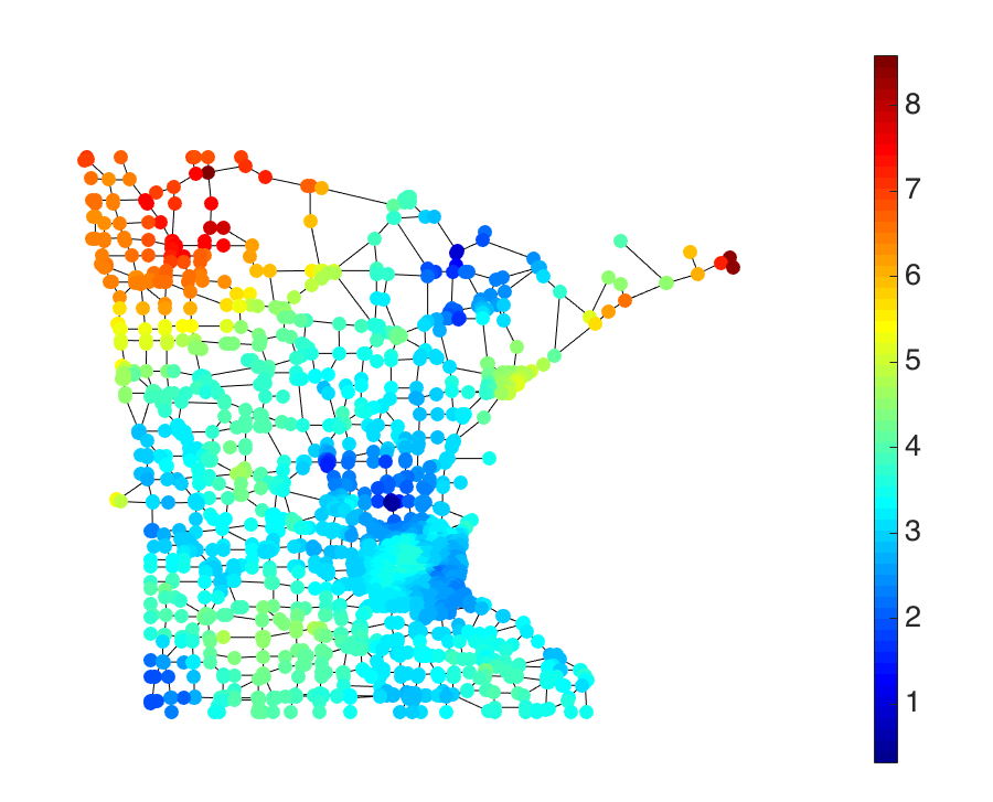
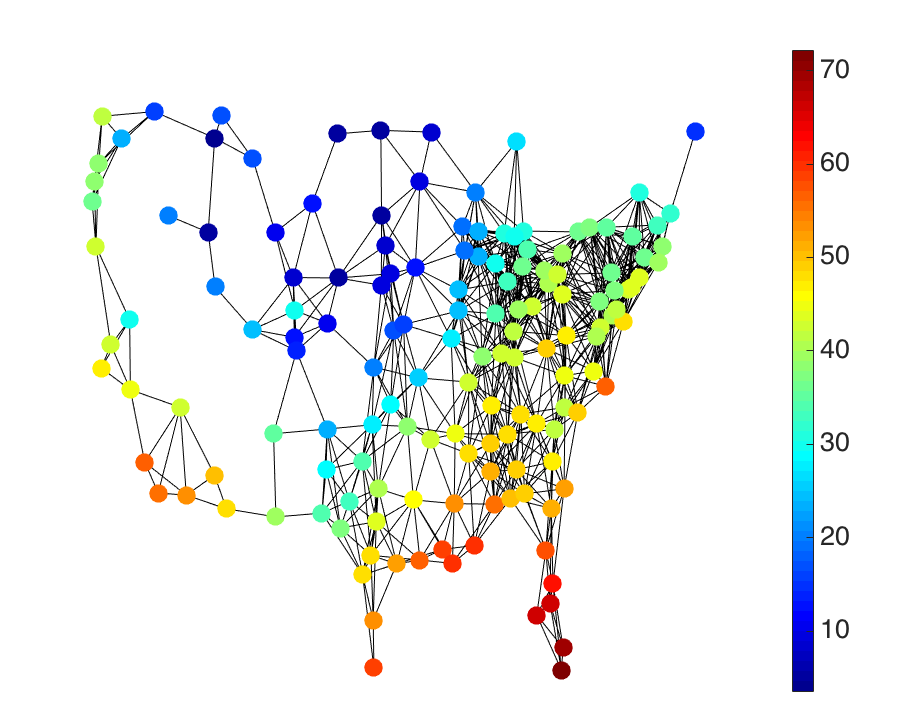
The approximately bandlimited class allows for a tail after the first K𝐾K frequency components, whose shape and decay are controlled by μ𝜇\mu and β𝛽\beta; the smaller the μ𝜇\mu, the less energy from the high-frequency components is allowed in the tail, and the larger the β𝛽\beta, the higher the penalty on the energy from those high-frequency components. The class of ABLA(K)subscriptABLA𝐾\operatorname{ABL}_{\operatorname{A}}(K) is similar to the ellipsoid constraints in previous literature [51], where all the frequency components are considered in the constraints; in other words, ABLA(K)subscriptABLA𝐾\operatorname{ABL}_{\operatorname{A}}(K) poses fewer restrictions on the low-frequency components. Many real graph signals exhibit the approximately bandlimited property; for example, Figures 1 and 2 show that the temperature readings across the U.S and wind speeds across Minnesota are approximately bandlimited graph signals. We have found that the approximately bandlimited class is more powerful than the bandlimited class when representing real graph signals.
Refer to caption Refer to caption
(a) Temperature. (b) Frequency content.
Figure 1: Temperature readings across the U.S is an approximately bandlimited graph signal. After the first ten frequency components (black dashed line), energy decays fast.
Refer to caption Refer to caption
(a) Wind. (b) Frequency content.
Figure 2: Wind speed across Minnesota is an approximately bandlimited graph signal. After the first 100 frequency components ( black dashed line), energy decays fast.

The following theorem details the relationship between ABLA(K,β,μ)subscriptABLA𝐾𝛽𝜇\operatorname{ABL}_{\operatorname{A}}(K,\beta,\mu) and GSA(η)subscriptGSA𝜂\operatorname{GS}_{\operatorname{A}}(\eta).

Theorem 2.

With β1𝛽1\beta\geq 1, μ,η0𝜇𝜂0\mu,\eta\geq 0 and K{0,1,,N1}𝐾01𝑁1K\in\{0,1,\cdots,N-1\},

  • ABLA(K,β,μ)subscriptABLA𝐾𝛽𝜇\operatorname{ABL}_{\operatorname{A}}(K,\beta,\mu) is a subset of GSA(η)subscriptGSA𝜂\operatorname{GS}_{\operatorname{A}}(\eta), when

    η(1λK1+4μ(1+K2β))2;𝜂superscript1subscript𝜆𝐾14𝜇1superscript𝐾2𝛽2\eta\geq\left(1-\lambda_{K-1}+\sqrt{\frac{4\mu}{(1+K^{2\beta})}}\right)^{2};
  • GSA(η)subscriptGSA𝜂\operatorname{GS}_{\operatorname{A}}(\eta) is a subset of ABLA(K,β,μ)subscriptABLA𝐾𝛽𝜇\operatorname{ABL}_{\operatorname{A}}(K,\beta,\mu), when

    μ1+(N1)2β1λKη.𝜇1superscript𝑁12𝛽1subscript𝜆𝐾𝜂\mu\geq\frac{1+(N-1)^{2\beta}}{1-\lambda_{K}}\eta.

From Theorem 2, we see that depending on the parameters, GSA(η)subscriptGSA𝜂\operatorname{GS}_{\operatorname{A}}(\eta) can be a subset of ABLA(K,β,μ)subscriptABLA𝐾𝛽𝜇\operatorname{ABL}_{\operatorname{A}}(K,\beta,\mu) or vice versa.

Proof.

To show when ABLA(K,β,μ)GSA(η)subscriptABLA𝐾𝛽𝜇subscriptGSA𝜂\operatorname{ABL}_{\operatorname{A}}(K,\beta,\mu)\subseteq\operatorname{GS}_{\operatorname{A}}(\eta), let 𝐱ABLA(K,β,μ)𝐱subscriptABLA𝐾𝛽𝜇\mathbf{x}\in\operatorname{ABL}_{\operatorname{A}}(K,\beta,\mu). Then,

𝐱A𝐱=k=0N1x^k𝐯kAk=0N1x^k𝐯knorm𝐱A𝐱normsuperscriptsubscript𝑘0𝑁1subscript^𝑥𝑘subscript𝐯𝑘Asuperscriptsubscript𝑘0𝑁1subscript^𝑥𝑘subscript𝐯𝑘\displaystyle\left\|\mathbf{x}-\operatorname{A}\mathbf{x}\right\|=\left\|\sum_{k=0}^{N-1}\widehat{x}_{k}\mathbf{v}_{k}-\operatorname{A}\sum_{k=0}^{N-1}\widehat{x}_{k}\mathbf{v}_{k}\right\|
(a)superscript𝑎\displaystyle\stackrel{{\scriptstyle(a)}}{{\leq}} k=0K1x^k𝐯kAk=0K1x^k𝐯knormsuperscriptsubscript𝑘0𝐾1subscript^𝑥𝑘subscript𝐯𝑘Asuperscriptsubscript𝑘0𝐾1subscript^𝑥𝑘subscript𝐯𝑘\displaystyle\left\|\sum_{k=0}^{K-1}\widehat{x}_{k}\mathbf{v}_{k}-\operatorname{A}\sum_{k=0}^{K-1}\widehat{x}_{k}\mathbf{v}_{k}\right\|
+k=KN1x^k𝐯kAk=KN1x^k𝐯knormsuperscriptsubscript𝑘𝐾𝑁1subscript^𝑥𝑘subscript𝐯𝑘Asuperscriptsubscript𝑘𝐾𝑁1subscript^𝑥𝑘subscript𝐯𝑘\displaystyle+\left\|\sum_{k=K}^{N-1}\widehat{x}_{k}\mathbf{v}_{k}-\operatorname{A}\sum_{k=K}^{N-1}\widehat{x}_{k}\mathbf{v}_{k}\right\|
(b)superscript𝑏\displaystyle\stackrel{{\scriptstyle(b)}}{{\leq}} (1λK1)𝐱+k=KN1x^k𝐯kAk=KN1x^k𝐯k1subscript𝜆𝐾1norm𝐱normsuperscriptsubscript𝑘𝐾𝑁1subscript^𝑥𝑘subscript𝐯𝑘Asuperscriptsubscript𝑘𝐾𝑁1subscript^𝑥𝑘subscript𝐯𝑘\displaystyle(1-\lambda_{K-1})\left\|\mathbf{x}\right\|+\left\|\sum_{k=K}^{N-1}\widehat{x}_{k}\mathbf{v}_{k}-\operatorname{A}\sum_{k=K}^{N-1}\widehat{x}_{k}\mathbf{v}_{k}\right\|
=(c)superscript𝑐\displaystyle\stackrel{{\scriptstyle(c)}}{{=}} (1λK1)𝐱+k=KN1(1λk)x^k𝐯k1subscript𝜆𝐾1norm𝐱normsuperscriptsubscript𝑘𝐾𝑁11subscript𝜆𝑘subscript^𝑥𝑘subscript𝐯𝑘\displaystyle(1-\lambda_{K-1})\left\|\mathbf{x}\right\|+\left\|\sum_{k=K}^{N-1}(1-\lambda_{k})\widehat{x}_{k}\mathbf{v}_{k}\right\|
=(d)superscript𝑑\displaystyle\stackrel{{\scriptstyle(d)}}{{=}} (1λK1)𝐱+k=KN1(1λk)2x^k21subscript𝜆𝐾1norm𝐱superscriptsubscript𝑘𝐾𝑁1superscript1subscript𝜆𝑘2superscriptsubscript^𝑥𝑘2\displaystyle(1-\lambda_{K-1})\left\|\mathbf{x}\right\|+\sqrt{\sum_{k=K}^{N-1}(1-\lambda_{k})^{2}\widehat{x}_{k}^{2}}
=\displaystyle= (1λK1)𝐱+k=KN1(1λk)2(1+k2β)(1+k2β)x^k21subscript𝜆𝐾1norm𝐱superscriptsubscript𝑘𝐾𝑁1superscript1subscript𝜆𝑘21superscript𝑘2𝛽1superscript𝑘2𝛽superscriptsubscript^𝑥𝑘2\displaystyle(1-\lambda_{K-1})\left\|\mathbf{x}\right\|+\sqrt{\sum_{k=K}^{N-1}\frac{(1-\lambda_{k})^{2}}{(1+k^{2\beta})}(1+k^{2\beta})\widehat{x}_{k}^{2}}
\displaystyle\leq (1λK1)𝐱+limit-from1subscript𝜆𝐾1norm𝐱\displaystyle(1-\lambda_{K-1})\left\|\mathbf{x}\right\|+
+\displaystyle+ (maxk{K,,N1}(1λk)2(1+k2β))k=KN1(1+k2β)x^k2subscript𝑘𝐾𝑁1superscript1subscript𝜆𝑘21superscript𝑘2𝛽superscriptsubscript𝑘𝐾𝑁11superscript𝑘2𝛽superscriptsubscript^𝑥𝑘2\displaystyle\sqrt{\left(\max_{k\in\{K,\cdots,N-1\}}\frac{(1-\lambda_{k})^{2}}{(1+k^{2\beta})}\right)\sum_{k=K}^{N-1}(1+k^{2\beta})\widehat{x}_{k}^{2}}
(e)superscript𝑒\displaystyle\stackrel{{\scriptstyle(e)}}{{\leq}} (1λK1)𝐱+4(1+K2β)k=KN1(1+k2β)x^k21subscript𝜆𝐾1norm𝐱41superscript𝐾2𝛽superscriptsubscript𝑘𝐾𝑁11superscript𝑘2𝛽superscriptsubscript^𝑥𝑘2\displaystyle(1-\lambda_{K-1})\left\|\mathbf{x}\right\|+\sqrt{\frac{4}{(1+K^{2\beta})}\sum_{k=K}^{N-1}(1+k^{2\beta})\widehat{x}_{k}^{2}}
(f)superscript𝑓\displaystyle\stackrel{{\scriptstyle(f)}}{{\leq}} (1λK1+4μ(1+K2β))𝐱,1subscript𝜆𝐾14𝜇1superscript𝐾2𝛽norm𝐱\displaystyle\left(1-\lambda_{K-1}+\sqrt{\frac{4\mu}{(1+K^{2\beta})}}\right)\left\|\mathbf{x}\right\|,

where (a) follows from the triangle inequality; (b) from Theorem 1; (c) from A𝐯k=λk𝐯kAsubscript𝐯𝑘subscript𝜆𝑘subscript𝐯𝑘\operatorname{A}\mathbf{v}_{k}=\lambda_{k}\mathbf{v}_{k}; (d) from the fact that Vα2=α2subscriptnormV𝛼2subscriptnorm𝛼2\left\|\operatorname{V}\alpha\right\|_{2}=\|\alpha\|_{2} by Parseval’s equality since VV\operatorname{V} is orthonormal, with αi=(1λi)x^isubscript𝛼𝑖1subscript𝜆𝑖subscript^𝑥𝑖\alpha_{i}=(1-\lambda_{i})\widehat{x}_{i}, for i=K,K+1,,N1𝑖𝐾𝐾1𝑁1i=K,\,K+1,\,\ldots,\,N-1 and 00 otherwise; (e) from 1λK11subscript𝜆𝐾1-1\leq\lambda_{K}\leq 1; and (f) from 𝐱ABLA(K,β,μ)𝐱subscriptABLA𝐾𝛽𝜇\mathbf{x}\in\operatorname{ABL}_{\operatorname{A}}(K,\beta,\mu).

To show the second statement when GSA(η)ABLA(K,β,μ)subscriptGSA𝜂subscriptABLA𝐾𝛽𝜇\operatorname{GS}_{\operatorname{A}}(\eta)\subseteq\operatorname{ABL}_{\operatorname{A}}(K,\beta,\mu), let 𝐱GSA(η)𝐱subscriptGSA𝜂\mathbf{x}\in\operatorname{GS}_{\operatorname{A}}(\eta). Then,

k=KN1(1+k2β)x^k2=k=KN11+k2β(1λk)2(1λk)2x^k2superscriptsubscript𝑘𝐾𝑁11superscript𝑘2𝛽superscriptsubscript^𝑥𝑘2superscriptsubscript𝑘𝐾𝑁11superscript𝑘2𝛽superscript1subscript𝜆𝑘2superscript1subscript𝜆𝑘2superscriptsubscript^𝑥𝑘2\displaystyle\sum_{k=K}^{N-1}(1+k^{2\beta})\widehat{x}_{k}^{2}=\sum_{k=K}^{N-1}\frac{1+k^{2\beta}}{(1-\lambda_{k})^{2}}(1-\lambda_{k})^{2}\widehat{x}_{k}^{2}
\displaystyle\leq (maxk{K,,N1}1+k2β(1λk)2)k=KN1(1λk)2x^k2subscript𝑘𝐾𝑁11superscript𝑘2𝛽superscript1subscript𝜆𝑘2superscriptsubscript𝑘𝐾𝑁1superscript1subscript𝜆𝑘2superscriptsubscript^𝑥𝑘2\displaystyle\left(\max_{k\in\{K,\cdots,N-1\}}\frac{1+k^{2\beta}}{(1-\lambda_{k})^{2}}\right)\sum_{k=K}^{N-1}(1-\lambda_{k})^{2}\widehat{x}_{k}^{2}
=\displaystyle= 1+(N1)2β(1λK)2k=KN1(1λk)2x^k21superscript𝑁12𝛽superscript1subscript𝜆𝐾2superscriptsubscript𝑘𝐾𝑁1superscript1subscript𝜆𝑘2superscriptsubscript^𝑥𝑘2\displaystyle\frac{1+(N-1)^{2\beta}}{(1-\lambda_{K})^{2}}\sum_{k=K}^{N-1}(1-\lambda_{k})^{2}\widehat{x}_{k}^{2}
(a)superscript𝑎\displaystyle\stackrel{{\scriptstyle(a)}}{{\leq}} 1+(N1)2β(1λK)2η𝐱2,1superscript𝑁12𝛽superscript1subscript𝜆𝐾2𝜂superscriptnorm𝐱2\displaystyle\frac{1+(N-1)^{2\beta}}{(1-\lambda_{K})^{2}}\eta\left\|\mathbf{x}\right\|^{2},

where (a) follows from k=KN1(1λk)2x^k2k=0N1(1λk)2x^k2=𝐱A𝐱22η𝐱22superscriptsubscript𝑘𝐾𝑁1superscript1subscript𝜆𝑘2superscriptsubscript^𝑥𝑘2superscriptsubscript𝑘0𝑁1superscript1subscript𝜆𝑘2superscriptsubscript^𝑥𝑘2superscriptsubscriptnorm𝐱A𝐱22𝜂superscriptsubscriptnorm𝐱22\sum_{k=K}^{N-1}(1-\lambda_{k})^{2}\widehat{x}_{k}^{2}\leq\sum_{k=0}^{N-1}(1-\lambda_{k})^{2}\widehat{x}_{k}^{2}=\left\|\mathbf{x}-\operatorname{A}\mathbf{x}\right\|_{2}^{2}\leq\eta\left\|\mathbf{x}\right\|_{2}^{2}, where the last inequality follows from Definition 1. ∎

From Theorem 2, we see that ABLA(K,β,μ)subscriptABLA𝐾𝛽𝜇\operatorname{ABL}_{\operatorname{A}}(K,\beta,\mu) is not only more general than BLA(K)subscriptBLA𝐾\operatorname{BL}_{\operatorname{A}}(K), but describes GSA(η)subscriptGSA𝜂\operatorname{GS}_{\operatorname{A}}(\eta) in a more controlled fashion. In this paper, we focus on ABLA(K,β,μ)subscriptABLA𝐾𝛽𝜇\operatorname{ABL}_{\operatorname{A}}(K,\beta,\mu), and study the recovery performance of this class under three sampling strategies.

III-B Sampling & Recovery Strategies

We consider the procedure of sampling and recovery as follows: we sample m𝑚m coefficients from a graph signal 𝐱N𝐱superscript𝑁\mathbf{x}\in\mathbb{R}^{N} with noise to produce a noisy sampled signal 𝐲m𝐲superscript𝑚\mathbf{y}\in\mathbb{R}^{m}, that is,

𝐲𝐲\displaystyle\mathbf{y} =\displaystyle= Ψ𝐱+ϵ𝐱+ϵ,Ψ𝐱italic-ϵsubscript𝐱italic-ϵ\displaystyle\Psi\mathbf{x}+\epsilon\ \equiv\ \mathbf{x}_{\mathcal{M}}+\epsilon, (7)

where ϵ𝒩(0,σ2Im×m)similar-toitalic-ϵ𝒩0superscript𝜎2subscriptI𝑚𝑚\epsilon\sim\mathcal{N}(0,\sigma^{2}\operatorname{I}_{m\times m}), and =(1,,m)subscript1subscript𝑚\mathcal{M}=(\mathcal{M}_{1},\ldots,\mathcal{M}_{m}) denotes the sequence of sample indices called the sampling set, with i{0,1,,N1}subscript𝑖01𝑁1\mathcal{M}_{i}\in\{0,1,\cdots,N-1\}, ||=m𝑚|\mathcal{M}|=m and the sampling operator ΨΨ\Psi is a linear mapping from Nsuperscript𝑁\mathbb{R}^{N} to msuperscript𝑚\mathbb{R}^{m}, defined as

Ψi,j={1,j=i;0,otherwise.subscriptΨ𝑖𝑗cases1𝑗subscript𝑖0otherwise\Psi_{i,j}=\left\{\begin{array}[]{rl}1,&j=\mathcal{M}_{i};\\ 0,&\mbox{otherwise}.\end{array}\right. (8)

We then interpolate 𝐲𝐲\mathbf{y} to get 𝐱Nsuperscript𝐱superscript𝑁\mathbf{x}^{*}\in\mathbb{R}^{N}, which recovers 𝐱𝐱\mathbf{x} either exactly or approximately.

We consider three different sampling strategies:

  • uniform sampling means that sample indices are chosen from {0,1,,N1}01𝑁1\{0,1,\ldots,N-1\} independently and randomly;

  • experimentally designed sampling means that sample indices can be chosen beforehand; and

  • active sampling means that sample indices can be chosen as a function of the sample points and the samples collected up to that instance, that is, isubscript𝑖\mathcal{M}_{i} depends only on {j,yj}j<isubscriptsubscript𝑗subscript𝑦𝑗𝑗𝑖\{\mathcal{M}_{j},y_{j}\}_{j<i}.

It is clear that uniform sampling is a subset of experimentally designed sampling, which is again a subset of active sampling.

The goal in this paper is to study the fundamental limitations of these three sampling strategies when recovering approximately bandlimited graph signals. This study is related to many real-world applications. For example, in semi-supervised learning, datasets are modeled as a graph with data samples as nodes and similarities between those data samples as edges. Features and labels associated with data samples form approximately bandlimited graph signals. We aim to select data samples as labeled data and recover the labels for the unlabeled data. The sampling strategy helps select the most informative data samples and minimizes the recovery error. Some other applications include route planning based on wind speed [52], sensor position selection [53] and compressive spectral clustering [54].

IV Fundamental Limits of Sampling Strategies

In this section, we study the fundamental limitations of the three sampling strategies for recovering ABLA(K,β,μ)subscriptABLA𝐾𝛽𝜇\operatorname{ABL}_{\operatorname{A}}(K,\beta,\mu) by showing minimax lower bounds. We do this by following the minimax decision rule and finding tight lower bounds for the minimax risk over all possible recovery strategies [55]. In other words, we try to minimize the recovery error in the worst case and use a tight lower bound to describe this minimax error.

We start by introducing some notation [46].

Definition 4.

For a recovery strategy (𝐱,)superscript𝐱(\mathbf{x}^{*},\mathcal{M}), and a vector 𝐱N𝐱superscript𝑁\mathbf{x}\in\mathbb{R}^{N}, the recovery strategy risk is

R(𝐱,,𝐱)=𝔼𝐱,[d2(𝐱,𝐱)],𝑅superscript𝐱𝐱subscript𝔼𝐱delimited-[]superscript𝑑2superscript𝐱𝐱R(\mathbf{x}^{*},\mathcal{M},\mathbf{x})\ =\ \mathbb{E}_{\mathbf{x},\mathcal{M}}[d^{2}(\mathbf{x}^{*},\mathbf{x})],

where 𝔼𝐱,subscript𝔼𝐱\mathbb{E}_{\mathbf{x},\mathcal{M}} is the expectation with respect to the probability measure of {xi,yi}isubscriptsubscript𝑥𝑖subscript𝑦𝑖𝑖\{x_{i},y_{i}\}_{i\in\mathcal{M}} and d(𝐱,𝐱)𝑑superscript𝐱𝐱d(\mathbf{x}^{*},\mathbf{x}) is the error metric. Here we use the 2subscript2\ell_{2} norm 𝐱𝐱2subscriptnormsuperscript𝐱𝐱2\left\|\mathbf{x}^{*}-\mathbf{x}\right\|_{2}. The maximum risk of a recovery strategy is sup𝐱NR(𝐱,,𝐱)subscriptsupremum𝐱superscript𝑁𝑅superscript𝐱𝐱\sup_{\mathbf{x}\in\mathbb{R}^{N}}R(\mathbf{x}^{*},\mathcal{M},\mathbf{x}).

The lower bounds we present will be of the form

inf(𝐱,)Θsup𝐱N𝔼𝐱,[d2(𝐱,𝐱)]cϕm2, for all mm0,formulae-sequencesubscriptinfimumsuperscript𝐱Θsubscriptsupremum𝐱superscript𝑁subscript𝔼𝐱delimited-[]superscript𝑑2superscript𝐱𝐱𝑐superscriptsubscriptitalic-ϕ𝑚2 for all 𝑚subscript𝑚0\inf_{(\mathbf{x}^{*},\mathcal{M})\in\Theta}\sup_{\mathbf{x}\in\mathbb{R}^{N}}\mathbb{E}_{\mathbf{x},\mathcal{M}}[d^{2}(\mathbf{x}^{*},\mathbf{x})]\geq c\phi_{m}^{2},\text{ for all }m\geq m_{0}, (9)

where infinfimum\inf is the infimum (greatest lower bound) and supsupremum\sup is the supremum (least upper bound), m𝑚m is the number of samples, m0subscript𝑚0m_{0}\in\mathbb{N}, c>0𝑐0c>0 is a constant, ϕmsubscriptitalic-ϕ𝑚\phi_{m} is a positive sequence converging to zero, and ΘΘ\Theta is the set of all recovery strategies. The sequence ϕm2superscriptsubscriptitalic-ϕ𝑚2\phi_{m}^{2} is denoted as a lower rate of convergence.

The upper bounds on the maximum risk are usually obtained through explicit recovery strategies, as will be shown in Section V. The upper bounds we present will be of the form

inf(𝐱,)Θsup𝐱N𝔼𝐱,[d2(𝐱,𝐱)]Cϕm2, for all mm0,formulae-sequencesubscriptinfimumsuperscript𝐱Θsubscriptsupremum𝐱superscript𝑁subscript𝔼𝐱delimited-[]superscript𝑑2superscript𝐱𝐱𝐶superscriptsubscriptitalic-ϕ𝑚2 for all 𝑚subscript𝑚0\inf_{(\mathbf{x}^{*},\mathcal{M})\in\Theta}\sup_{\mathbf{x}\in\mathbb{R}^{N}}\mathbb{E}_{\mathbf{x},\mathcal{M}}[d^{2}(\mathbf{x}^{*},\mathbf{x})]\leq C\phi_{m}^{2},\text{ for all }m\geq m_{0}, (10)

where C>0𝐶0C>0 is a constant. If (9) and (10) both hold, then ϕmsubscriptitalic-ϕ𝑚\phi_{m} is said to be the optimal rate of convergence and there is no recovery strategy that asymptotically outperforms the proposed one. When talking about optimal rates of convergence, we bound the sequence by a polynomial and make statements of the form: Given γ1<γ<γ2subscript𝛾1𝛾subscript𝛾2\gamma_{1}<\gamma<\gamma_{2}, a rate of convergence ϕm2superscriptsubscriptitalic-ϕ𝑚2\phi_{m}^{2} is equivalent to mγsuperscript𝑚𝛾m^{-\gamma} if and only if mγ2<ϕm2<mγ1superscript𝑚subscript𝛾2superscriptsubscriptitalic-ϕ𝑚2superscript𝑚subscript𝛾1m^{-\gamma_{2}}<\phi_{m}^{2}<m^{-\gamma_{1}} for n𝑛n large enough.

Note that the general bounds are for arbitrary graphs and thus involve parameters that depend on the graph structure; given the graph structure, we can specify the parameters and show explicit rates of convergence, as we will do in Section VI.

Let V(2,K)subscriptV2𝐾\operatorname{V}_{(2,K)} be the sub-matrix of VV\operatorname{V}, consisting of the K𝐾Kth to the (2K1)2𝐾1(2K-1)th columns of VV\operatorname{V}.

Theorem 3.

Given the class ABLA(K,β,μ)subscriptABLA𝐾𝛽𝜇\operatorname{ABL}_{\operatorname{A}}(K,\beta,\mu):
(1) Under uniform sampling,

inf(𝐱,)Θusup𝐱ABLA(K,β,μ)𝔼𝐱,(𝐱𝐱22𝐱22)subscriptinfimumsuperscript𝐱subscriptΘusubscriptsupremum𝐱subscriptABLA𝐾𝛽𝜇subscript𝔼𝐱superscriptsubscriptnormsuperscript𝐱𝐱22superscriptsubscriptnorm𝐱22\displaystyle\inf_{(\mathbf{x}^{*},\mathcal{M})\in\Theta_{\rm u}}\sup_{\mathbf{x}\in\operatorname{ABL}_{\operatorname{A}}(K,\beta,\mu)}\mathbb{E}_{\mathbf{x},\mathcal{M}}\left(\frac{\left\|\mathbf{x}^{*}-\mathbf{x}\right\|_{2}^{2}}{\left\|\mathbf{x}\right\|_{2}^{2}}\right)
\displaystyle\geq maxKκ0Nc1μκ02β(1cμ𝐱22σ2κ02β+2NV(2,κ0)F2m),subscript𝐾subscript𝜅0𝑁subscript𝑐1𝜇superscriptsubscript𝜅02𝛽1𝑐𝜇superscriptsubscriptnorm𝐱22superscript𝜎2superscriptsubscript𝜅02𝛽2𝑁superscriptsubscriptnormsubscriptV2subscript𝜅0𝐹2𝑚\displaystyle\max_{K\leq\kappa_{0}\leq N}\frac{c_{1}\mu}{\kappa_{0}^{2\beta}}\left(1-\frac{c\mu\left\|\mathbf{x}\right\|_{2}^{2}}{\sigma^{2}\kappa_{0}^{2\beta+2}N}\left\|\operatorname{V}_{(2,\kappa_{0})}\right\|_{F}^{2}m\right),

where c1>0subscript𝑐10c_{1}>0 , 0<c<10𝑐10<c<1, and ΘusubscriptΘu\Theta_{\rm u} denotes the set of all recovery strategies based on uniform sampling;
(2) Under experimentally designed sampling,

inf(𝐱,)Θesup𝐱ABLA(K,β,μ)𝔼𝐱,(𝐱𝐱22𝐱22)subscriptinfimumsuperscript𝐱subscriptΘesubscriptsupremum𝐱subscriptABLA𝐾𝛽𝜇subscript𝔼𝐱superscriptsubscriptnormsuperscript𝐱𝐱22superscriptsubscriptnorm𝐱22\displaystyle\inf_{(\mathbf{x}^{*},\mathcal{M})\in\Theta_{\rm e}}\sup_{\mathbf{x}\in\operatorname{ABL}_{\operatorname{A}}(K,\beta,\mu)}\mathbb{E}_{\mathbf{x},\mathcal{M}}\left(\frac{\left\|\mathbf{x}^{*}-\mathbf{x}\right\|_{2}^{2}}{\left\|\mathbf{x}\right\|_{2}^{2}}\right)
\displaystyle\geq maxKκ0Nc1μκ02β(1cμ𝐱22σ2κ02β+2V(2,κ0),22m),subscript𝐾subscript𝜅0𝑁subscript𝑐1𝜇superscriptsubscript𝜅02𝛽1𝑐𝜇superscriptsubscriptnorm𝐱22superscript𝜎2superscriptsubscript𝜅02𝛽2superscriptsubscriptnormsubscriptV2subscript𝜅022𝑚\displaystyle\max_{K\leq\kappa_{0}\leq N}\frac{c_{1}\mu}{\kappa_{0}^{2\beta}}\left(1-\frac{c\mu\left\|\mathbf{x}\right\|_{2}^{2}}{\sigma^{2}\kappa_{0}^{2\beta+2}}\left\|\operatorname{V}_{(2,\kappa_{0})}\right\|_{\infty,2}^{2}m\right),

where c1>0subscript𝑐10c_{1}>0 , 0<c<10𝑐10<c<1, and ΘesubscriptΘe\Theta_{\rm e} denotes the set of all recovery strategies based on experimentally designed sampling;
(3) Under active sampling,

inf(𝐱,)Θasup𝐱ABLA(K,β,μ)𝔼𝐱,(𝐱𝐱22𝐱22)subscriptinfimumsuperscript𝐱subscriptΘasubscriptsupremum𝐱subscriptABLA𝐾𝛽𝜇subscript𝔼𝐱superscriptsubscriptnormsuperscript𝐱𝐱22superscriptsubscriptnorm𝐱22\displaystyle\inf_{(\mathbf{x}^{*},\mathcal{M})\in\Theta_{\rm a}}\sup_{\mathbf{x}\in\operatorname{ABL}_{\operatorname{A}}(K,\beta,\mu)}\mathbb{E}_{\mathbf{x},\mathcal{M}}\left(\frac{\left\|\mathbf{x}^{*}-\mathbf{x}\right\|_{2}^{2}}{\left\|\mathbf{x}\right\|_{2}^{2}}\right)
\displaystyle\geq maxKκ0Nc1μκ02β(1cμ𝐱22σ2κ02β+2V(2,κ0),22m),subscript𝐾subscript𝜅0𝑁subscript𝑐1𝜇superscriptsubscript𝜅02𝛽1𝑐𝜇superscriptsubscriptnorm𝐱22superscript𝜎2superscriptsubscript𝜅02𝛽2superscriptsubscriptnormsubscriptV2subscript𝜅022𝑚\displaystyle\max_{K\leq\kappa_{0}\leq N}\frac{c_{1}\mu}{\kappa_{0}^{2\beta}}\left(1-\frac{c\mu\left\|\mathbf{x}\right\|_{2}^{2}}{\sigma^{2}\kappa_{0}^{2\beta+2}}\left\|\operatorname{V}_{(2,\kappa_{0})}\right\|_{\infty,2}^{2}m\right),

where c1>0subscript𝑐10c_{1}>0 , 0<c<10𝑐10<c<1, and ΘasubscriptΘa\Theta_{\rm a} denotes the set of all recovery strategies based on active sampling.

See Appendix A in the supporting document for the proof of these results. From Theorem 3, we see that experimentally designed sampling has the same minimax lower bound as active sampling, which means that collecting the feedback before taking samples does not fundamentally improve the recovery performance. We also see that the three minimax lower bounds depend on the properties of V(2,κ0)subscriptV2subscript𝜅0\operatorname{V}_{(2,\kappa_{0})}, which depend on the graph structure. When each row of V(2,κ0)subscriptV2subscript𝜅0\operatorname{V}_{(2,\kappa_{0})} has roughly similar energy, V(2,κ0)F2superscriptsubscriptnormsubscriptV2subscript𝜅0𝐹2\left\|\operatorname{V}_{(2,\kappa_{0})}\right\|_{F}^{2} and NV(2,κ0),22𝑁superscriptsubscriptnormsubscriptV2subscript𝜅022N\left\|\operatorname{V}_{(2,\kappa_{0})}\right\|_{\infty,2}^{2} are similar; when the energy is concentrated in a few rows, NV(2,κ0),22𝑁superscriptsubscriptnormsubscriptV2subscript𝜅022N\left\|\operatorname{V}_{(2,\kappa_{0})}\right\|_{\infty,2}^{2} is much larger than V(2,κ0)F2superscriptsubscriptnormsubscriptV2subscript𝜅0𝐹2\left\|\operatorname{V}_{(2,\kappa_{0})}\right\|_{F}^{2}; in other words, the minimax lower bound for experimentally designed sampling is tighter than that for uniform sampling. This happens in many real-world graphs that have complex, irregular structure. The minimax lower bounds thus show the potential advantage of experimentally designed sampling and active sampling over uniform sampling. We will elaborate on this in Sections VI and VII.

V Recovery Strategy

In the previous section, we presented the minimax lower bounds for each of the three sampling strategies and showed that active sampling cannot fundamentally perform better than experimentally designed sampling. We now propose a recovery strategy for both uniform sampling and experimentally designed sampling and evaluate its statistical properties.

V-A Algorithm

To analyze uniform sampling and experimentally designed sampling in a similar manner, we consider sampling score-based sampling that unifies both sampling strategies. Sampling score-based sampling means that the sample indices are chosen from an importance sampling distribution that is proportional to some sampling score. Let {πi}i=1Nsuperscriptsubscriptsubscript𝜋𝑖𝑖1𝑁\{\pi_{i}\}_{i=1}^{N} be a set of sampling scores, where πisubscript𝜋𝑖\pi_{i} denotes the probability to choose the i𝑖ith sample in each random trial. When the sampling score for each node is the same, we get uniform sampling; when the sampling score for each node is designed based on the graph structure, we get experimentally designed sampling.

For ABLA(K)subscriptABLA𝐾\operatorname{ABL}_{\operatorname{A}}(K), most of the energy is concentrated in the first K𝐾K frequency components and the graph signal can be approximately recovered by using those. We consider the following recovery strategy to estimate those frequency components by projecting samples onto the bandlimited space spanned by the first K𝐾K frequency components.

Algorithm 1.

We sample a graph signal m𝑚m times. Each time, we independently choose a node j=isubscript𝑗𝑖\mathcal{M}_{j}=i, j=1,,m𝑗1𝑚j=1,\ldots,m, with probability πisubscript𝜋𝑖\pi_{i}, and take a measurement yjsubscript𝑦subscript𝑗y_{\mathcal{M}_{j}}. Let Ψm×NΨsuperscript𝑚𝑁\Psi\in\mathbb{R}^{m\times N} be the sampling operator, V(K)N×KsubscriptV𝐾superscript𝑁𝐾\operatorname{V}_{(K)}\in\mathbb{R}^{N\times K} be the first K𝐾K columns of VV\operatorname{V}, and DN×NDsuperscript𝑁𝑁\operatorname{D}\in\mathbb{R}^{N\times N} be a diagonal rescaling matrix with Di,i=1/mπisubscriptD𝑖𝑖1𝑚subscript𝜋𝑖\operatorname{D}_{i,i}=1/\sqrt{m\pi_{i}}. We recover the original graph signal by solving the following optimization problem:

𝐱SPsubscriptsuperscript𝐱SP\displaystyle\mathbf{x}^{*}_{\rm SP} =\displaystyle= V(K)argmin𝐱^(K)ΨTΨD2ΨT𝐲V(K)𝐱^(K)22subscriptV𝐾subscriptsubscript^𝐱𝐾superscriptsubscriptnormsuperscriptΨ𝑇ΨsuperscriptD2superscriptΨ𝑇𝐲subscriptV𝐾subscript^𝐱𝐾22\displaystyle\operatorname{V}_{(K)}\arg\min_{\widehat{\mathbf{x}}_{(K)}}\left\|\Psi^{T}\Psi\operatorname{D}^{2}\Psi^{T}\mathbf{y}-\operatorname{V}_{(K)}\widehat{\mathbf{x}}_{(K)}\right\|_{2}^{2} (12)
=\displaystyle= V(K)U(K)ΨTΨD2ΨT𝐲,subscriptV𝐾subscriptU𝐾superscriptΨ𝑇ΨsuperscriptD2superscriptΨ𝑇𝐲\displaystyle\operatorname{V}_{(K)}\operatorname{U}_{(K)}\Psi^{T}\Psi\operatorname{D}^{2}\Psi^{T}\mathbf{y},

where 𝐲𝐲\mathbf{y} is a vector representation of the samples (7).

We call Algorithm 1 sampled projection (SampleProj) because we reweight and project the samples onto the bandlimited space. ΨT𝐲NsuperscriptΨ𝑇𝐲superscript𝑁\Psi^{T}\mathbf{y}\in\mathbb{R}^{N} rescales the sampled signal 𝐲m𝐲superscript𝑚\mathbf{y}\in\mathbb{R}^{m} through zero padding. The rescaling matrix D2superscriptD2\operatorname{D}^{2} compensates for non-uniform weights in sampling and equalizes samples from different sampling scores. The term ΨTΨD2ΨT𝐲superscriptΨ𝑇ΨsuperscriptD2superscriptΨ𝑇𝐲\Psi^{T}\Psi\operatorname{D}^{2}\Psi^{T}\mathbf{y} denotes the equalized and zero-padding samples. The objective function (LABEL:eq:SubsampleProj) minimizes the distance between our estimate and the samples. The intuition behind the solution (12) is that we project the equalized and zero-padding samples onto a bandlimited space spanned by V(K)subscriptV𝐾\operatorname{V}_{(K)} to remove aliasing. The term U(K)ΨTΨD2ΨT𝐲subscriptU𝐾superscriptΨ𝑇ΨsuperscriptD2superscriptΨ𝑇𝐲\operatorname{U}_{(K)}\Psi^{T}\Psi\operatorname{D}^{2}\Psi^{T}\mathbf{y} is an unbiased estimator for the first K𝐾K frequency components, which will be shown later. Thus, in expectation, the recovered graph signal 𝐱SPsubscriptsuperscript𝐱SP\mathbf{x}^{*}_{\rm SP} is a linear approximation of any graph signal 𝐱𝐱\mathbf{x}. When 𝐱𝐱\mathbf{x} is bandlimited, 𝐱SPsubscriptsuperscript𝐱SP\mathbf{x}^{*}_{\rm SP} perfectly recovers 𝐱𝐱\mathbf{x}; when 𝐱𝐱\mathbf{x} is approximately bandlimited, 𝐱SPsubscriptsuperscript𝐱SP\mathbf{x}^{*}_{\rm SP} has a bias due to the existence of high-frequency components.

It is also intuitive to consider the following recovery strategy [56],

𝐱LSsubscriptsuperscript𝐱LS\displaystyle\mathbf{x}^{*}_{\rm LS} =\displaystyle= V(K)argmin𝐱^(K)DΨT𝐲DΨTΨV(K)𝐱^(K)22subscriptV𝐾subscriptsubscript^𝐱𝐾superscriptsubscriptnormDsuperscriptΨ𝑇𝐲DsuperscriptΨ𝑇ΨsubscriptV𝐾subscript^𝐱𝐾22\displaystyle\operatorname{V}_{(K)}\arg\min_{\widehat{\mathbf{x}}_{(K)}}\left\|\operatorname{D}\Psi^{T}\mathbf{y}-\operatorname{D}\Psi^{T}\Psi\operatorname{V}_{(K)}\widehat{\mathbf{x}}_{(K)}\right\|_{2}^{2}
=\displaystyle= V(K)(D2ΨTΨV(K))DΨT𝐲,\displaystyle\operatorname{V}_{(K)}\left(\operatorname{D}^{2}\Psi^{T}\Psi\operatorname{V}_{(K)}\right)^{\dagger}\operatorname{D}\Psi^{T}\mathbf{y},

where we fit the sampled elements of the recovered graph signal to the samples by solving the least squares problem and ()superscript(\cdot)^{\dagger} is the pseudo-inverse operator [29]. The corresponding expected recovered graph signal is

𝔼𝐱LS=V(K)𝐱^(K)+V(K)PV(K)𝐱^(K),𝔼subscriptsuperscript𝐱LSsubscriptV𝐾subscript^𝐱𝐾subscriptV𝐾PsubscriptV𝐾subscript^𝐱𝐾\mathbb{E}\mathbf{x}^{*}_{\rm LS}=\operatorname{V}_{(K)}\widehat{\mathbf{x}}_{(K)}+\operatorname{V}_{(K)}\operatorname{P}\operatorname{V}_{(-K)}\widehat{\mathbf{x}}_{(-K)},

where P=(D2ΨTΨV(K))DPsuperscriptsuperscriptD2superscriptΨ𝑇ΨsubscriptV𝐾D\operatorname{P}=\left(\operatorname{D}^{2}\Psi^{T}\Psi\operatorname{V}_{(K)}\right)^{\dagger}\operatorname{D} ΨTΨ=(U(K)ΨTΨD2ΨTΨV(K))1superscriptΨ𝑇ΨsuperscriptsubscriptU𝐾superscriptΨ𝑇ΨsuperscriptD2superscriptΨ𝑇ΨsubscriptV𝐾1\Psi^{T}\Psi=\left(\operatorname{U}_{(K)}\Psi^{T}\Psi\operatorname{D}^{2}\Psi^{T}\Psi\operatorname{V}_{(K)}\right)^{-1} U(K)ΨTΨD2ΨTΨsubscriptU𝐾superscriptΨ𝑇ΨsuperscriptD2superscriptΨ𝑇Ψ\operatorname{U}_{(K)}\Psi^{T}\Psi\operatorname{D}^{2}\Psi^{T}\Psi, V(K)subscriptV𝐾\operatorname{V}_{(-K)} chooses the last K𝐾K columns of VV\operatorname{V}, and 𝐱^(K)subscript^𝐱𝐾\widehat{\mathbf{x}}_{(-K)} chooses the last K𝐾K columns of 𝐱𝐱\mathbf{x}. When 𝐱𝐱\mathbf{x} is bandlimited, 𝐱LSsubscriptsuperscript𝐱LS\mathbf{x}^{*}_{\rm LS} perfectly recovers 𝐱𝐱\mathbf{x}; when 𝐱𝐱\mathbf{x} is approximately bandlimited, however, 𝐱LSsubscriptsuperscript𝐱LS\mathbf{x}^{*}_{\rm LS} is a mixture of low-frequency and high-frequency components and it is hard to show its statistical properties. Moreover, it is less computationally efficient to compute 𝐱LSsubscriptsuperscript𝐱LS\mathbf{x}^{*}_{\rm LS} than 𝐱SPsubscriptsuperscript𝐱SP\mathbf{x}^{*}_{\rm SP} because of the presence of the inverse term.

Since the definitions of the bandlimited class and the approximately bandlimited class, and the proposed sampling strategies are all based on the graph Fourier transform instead of on graph shift, all the proposed methods work for other versions of the graph Fourier transform as well.

V-B Statistical Analysis

We study the statistical properties of Algorithm 1 by providing the bias, covariance, mean square error (MSE), and an optimal sampling distribution.

The following lemma shows that the sampled projection estimator is an unbiased estimator of the first K𝐾K frequency components for any sampling scores.

Lemma 1.

The sampled projection estimator with bandwidth K𝐾K and arbitrary sampling scores is an unbiased estimator of the first K𝐾K frequency components, that is,

𝔼𝐱=V(K)U(K)𝐱,for all 𝐱,𝔼superscript𝐱subscriptV𝐾subscriptU𝐾𝐱for all 𝐱\mathbb{E}\mathbf{x}^{*}\ =\ \operatorname{V}_{(K)}\operatorname{U}_{(K)}\mathbf{x},\quad\text{for all }\mathbf{x},

where 𝐱superscript𝐱\mathbf{x}^{*} is the solution of Algorithm 1.

Lemma 2 gives the exact covariance of the sampled projection estimator.

Lemma 2.

The covariance of sampled projection estimator 𝐱superscript𝐱\mathbf{x}^{*} has the following property:

Tr(Covar[𝐱])TrCovardelimited-[]superscript𝐱\displaystyle{\rm Tr}({\rm Covar}\left[\mathbf{x}^{*}\right]) =\displaystyle= 𝔼𝐱𝔼[𝐱]22𝔼superscriptsubscriptnormsuperscript𝐱𝔼delimited-[]superscript𝐱22\displaystyle\mathbb{E}\left\|\mathbf{x}^{*}-\mathbb{E}\left[\mathbf{x}^{*}\right]\right\|_{2}^{2}
=\displaystyle= Tr(U(K)WCV(K))1m𝐱^(K)22,TrsubscriptU𝐾subscriptW𝐶subscriptV𝐾1𝑚superscriptsubscriptnormsubscript^𝐱𝐾22\displaystyle{\rm Tr}\left(\operatorname{U}_{(K)}\operatorname{W}_{C}\operatorname{V}_{(K)}\right)-\frac{1}{m}\left\|\widehat{\mathbf{x}}_{(K)}\right\|_{2}^{2},

where Tr(\cdot) is the trace operator and WCsubscriptW𝐶\operatorname{W}_{C} is a diagonal matrix with (WC)i,i=(xi2+σ2)/(mπi)subscriptsubscriptW𝐶𝑖𝑖superscriptsubscript𝑥𝑖2superscript𝜎2𝑚subscript𝜋𝑖\left(\operatorname{W}_{C}\right)_{i,i}=(x_{i}^{2}+\sigma^{2})/(m\pi_{i}).

Theorem 4 shows the exact MSE of sampled projection estimator and an upper bound.

Theorem 4.

For 𝐱ABLA(K,β,μ)𝐱subscriptABLA𝐾𝛽𝜇\mathbf{x}\in\operatorname{ABL}_{\operatorname{A}}(K,\beta,\mu), let 𝐱superscript𝐱\mathbf{x}^{*} be the sampled projection estimator with bandwidth κK𝜅𝐾\kappa\geq K. Then,

𝔼𝐱𝐱22𝔼superscriptsubscriptnormsuperscript𝐱𝐱22\displaystyle\mathbb{E}\left\|\mathbf{x}^{*}-\mathbf{x}\right\|_{2}^{2} (13)
=\displaystyle= V(κ)𝐱^(κ)22+Tr(U(κ)WCV(κ))1m𝐱^(κ)22superscriptsubscriptnormsubscriptV𝜅subscript^𝐱𝜅22TrsubscriptU𝜅subscriptW𝐶subscriptV𝜅1𝑚superscriptsubscriptnormsubscript^𝐱𝜅22\displaystyle\left\|\operatorname{V}_{(-\kappa)}\widehat{\mathbf{x}}_{(-\kappa)}\right\|_{2}^{2}+{\rm Tr}\left(\operatorname{U}_{(\kappa)}\operatorname{W}_{C}\operatorname{V}_{(\kappa)}\right)-\frac{1}{m}\left\|\widehat{\mathbf{x}}_{(\kappa)}\right\|_{2}^{2}
\displaystyle\leq μ1+κ2β𝐱22+Tr(U(κ)WCV(κ)).𝜇1superscript𝜅2𝛽superscriptsubscriptnorm𝐱22TrsubscriptU𝜅subscriptW𝐶subscriptV𝜅\displaystyle\frac{\mu}{1+\kappa^{2\beta}}\left\|\mathbf{x}\right\|_{2}^{2}+{\rm Tr}\left(\operatorname{U}_{(\kappa)}\operatorname{W}_{C}\operatorname{V}_{(\kappa)}\right).

We merge the proofs of Lemmas 12 and Theorem 4 in Appendix B in the supporting document. The main idea follows from the bias-variance tradeoff. The bias term μ/(1+κ2β)𝐱22𝜇1superscript𝜅2𝛽superscriptsubscriptnorm𝐱22\mu/(1+\kappa^{2\beta})\left\|\mathbf{x}\right\|_{2}^{2} comes from the high-frequency components and Tr(U(κ)WCV(κ))TrsubscriptU𝜅subscriptW𝐶subscriptV𝜅{\rm Tr}\left(\operatorname{U}_{(\kappa)}\operatorname{W}_{C}\operatorname{V}_{(\kappa)}\right) comes from the covariance. The last inequality in Theorem 4 comes from relaxing the bias term and omitting a constant, which has nothing to do with the sampling scores. Thus, optimizing the upper bound over sampling scores is equivalent to optimizing the exact MSE.

We next study the MSEs of sampled projection estimator based on both uniform sampling and experimentally designed sampling.

Corollary 1.

The upper bound of MSE of uniform sampling is

𝔼𝐱𝐱22𝔼superscriptsubscriptnormsuperscript𝐱𝐱22\displaystyle\mathbb{E}\left\|\mathbf{x}^{*}-\mathbf{x}\right\|_{2}^{2} \displaystyle\leq μ1+κ2β𝐱22+Nmk=1κi=1NUk,i2(xi2+σ2).𝜇1superscript𝜅2𝛽superscriptsubscriptnorm𝐱22𝑁𝑚superscriptsubscript𝑘1𝜅superscriptsubscript𝑖1𝑁superscriptsubscriptU𝑘𝑖2superscriptsubscript𝑥𝑖2superscript𝜎2\displaystyle\frac{\mu}{1+\kappa^{2\beta}}\left\|\mathbf{x}\right\|_{2}^{2}+\frac{N}{m}\sum_{k=1}^{\kappa}\sum_{i=1}^{N}\operatorname{U}_{k,i}^{2}\left(x_{i}^{2}+\sigma^{2}\right).

The upper bound just specifies that the sampling score be πi=1/Nsubscript𝜋𝑖1𝑁\pi_{i}=1/N for all i𝑖i. For experimentally designed sampling, we are allowed to study the graph structure and design sample indices. In the following corollary, we show a set of optimal sampling scores of the sampled projection estimator by minimizing the upper bound of MSE.

Corollary 2.

The optimal sampling score of the sampled projection estimator with bandwidth κK𝜅𝐾\kappa\geq K is

πisubscript𝜋𝑖\displaystyle\pi_{i} proportional-to\displaystyle\propto (k=1κUk,i2)(xi2+σ2).superscriptsubscript𝑘1𝜅superscriptsubscriptU𝑘𝑖2superscriptsubscript𝑥𝑖2superscript𝜎2\displaystyle\sqrt{\left(\sum_{k=1}^{\kappa}\operatorname{U}_{k,i}^{2}\right)\left(x_{i}^{2}+\sigma^{2}\right)}.

The corresponding upper bound of MSE is

𝔼𝐱𝔼𝐱22𝔼superscriptsubscriptnormsuperscript𝐱𝔼superscript𝐱22\displaystyle\mathbb{E}\left\|\mathbf{x}^{*}-\mathbb{E}\mathbf{x}^{*}\right\|_{2}^{2}
\displaystyle\leq μ1+κ2β𝐱22+1m(i=1Nk=1κUk,i2(xi2+σ2))2.𝜇1superscript𝜅2𝛽superscriptsubscriptnorm𝐱221𝑚superscriptsuperscriptsubscript𝑖1𝑁superscriptsubscript𝑘1𝜅superscriptsubscriptU𝑘𝑖2superscriptsubscript𝑥𝑖2superscript𝜎22\displaystyle\frac{\mu}{1+\kappa^{2\beta}}\left\|\mathbf{x}\right\|_{2}^{2}+\frac{1}{m}\left(\sum_{i=1}^{N}\sqrt{\sum_{k=1}^{\kappa}\operatorname{U}_{k,i}^{2}\left(x_{i}^{2}+\sigma^{2}\right)}\right)^{2}.
Proof.

To obtain the optimal sampling score for the estimator, we minimize the MSE given in Theorem 4 and solve the following optimization problem.

minπiTr(U(κ)WCV(κ)),subscriptsubscript𝜋𝑖TrsubscriptU𝜅subscriptW𝐶subscriptV𝜅\displaystyle\min_{\pi_{i}}{\rm Tr}\left(\operatorname{U}_{(\kappa)}\operatorname{W}_{C}\operatorname{V}_{(\kappa)}\right),
subjecttoiπi=1,πi0.formulae-sequencesubjecttosubscript𝑖subscript𝜋𝑖1subscript𝜋𝑖0\displaystyle{\rm subject~{}to}~{}\sum_{i}\pi_{i}=1,\pi_{i}\geq 0.

The objective function is the variance term of the MSE derived in Theorem 4. Since the bias term has nothing to do with the sampling score, minimizing the variance term is equivalent to minimizing the MSE. The constraints require {πi}i=1Nsuperscriptsubscriptsubscript𝜋𝑖𝑖1𝑁\{\pi_{i}\}_{i=1}^{N} to be a valid probability distribution. The Lagrangian function is then

L(πi,η0,ηi)𝐿subscript𝜋𝑖subscript𝜂0subscript𝜂𝑖\displaystyle L(\pi_{i},\eta_{0},\eta_{i}) =\displaystyle= i=1N(xi2+σ2mπik=1κUk,i2)superscriptsubscript𝑖1𝑁superscriptsubscript𝑥𝑖2superscript𝜎2𝑚subscript𝜋𝑖superscriptsubscript𝑘1𝜅superscriptsubscriptU𝑘𝑖2\displaystyle\sum_{i=1}^{N}\left(\frac{x_{i}^{2}+\sigma^{2}}{m\pi_{i}}\sum_{k=1}^{\kappa}\operatorname{U}_{k,i}^{2}\right)
+η0(i=1Nπi1)+i=1Nηiπi,subscript𝜂0superscriptsubscript𝑖1𝑁subscript𝜋𝑖1superscriptsubscript𝑖1𝑁subscript𝜂𝑖subscript𝜋𝑖\displaystyle+\eta_{0}\left(\sum_{i=1}^{N}\pi_{i}-1\right)+\sum_{i=1}^{N}\eta_{i}\pi_{i},

where η0,ηisubscript𝜂0subscript𝜂𝑖\eta_{0},\eta_{i} are Lagrangian multipliers. We set the derivative of the Lagrangian function to zero,

dLdπi𝑑𝐿𝑑subscript𝜋𝑖\displaystyle\frac{dL}{d\pi_{i}} =\displaystyle= xi2+σ2mπl2k=1κUk,i2+η0+ηi=0,superscriptsubscript𝑥𝑖2superscript𝜎2𝑚superscriptsubscript𝜋𝑙2superscriptsubscript𝑘1𝜅superscriptsubscriptU𝑘𝑖2subscript𝜂0subscript𝜂𝑖0\displaystyle-\frac{x_{i}^{2}+\sigma^{2}}{m\pi_{l}^{2}}\sum_{k=1}^{\kappa}\operatorname{U}_{k,i}^{2}+\eta_{0}+\eta_{i}=0,

and obtain the optimal sampling score

πisubscript𝜋𝑖\displaystyle\pi_{i} proportional-to\displaystyle\propto (k=1κUk,i2)(xi2+σ2).superscriptsubscript𝑘1𝜅superscriptsubscriptU𝑘𝑖2superscriptsubscript𝑥𝑖2superscript𝜎2\displaystyle\sqrt{\left(\sum_{k=1}^{\kappa}\operatorname{U}_{k,i}^{2}\right)\left(x_{i}^{2}+\sigma^{2}\right)}. (14)

Substituting the optimal sampling score πisubscript𝜋𝑖\pi_{i} to the upper bound of the MSE (13),

𝔼𝐱𝔼𝐱22(a)μ1+κ2β𝐱22superscript𝑎𝔼superscriptsubscriptnormsuperscript𝐱𝔼superscript𝐱22𝜇1superscript𝜅2𝛽superscriptsubscriptnorm𝐱22\displaystyle\mathbb{E}\left\|\mathbf{x}^{*}-\mathbb{E}\mathbf{x}^{*}\right\|_{2}^{2}\ \stackrel{{\scriptstyle(a)}}{{\leq}}\ \frac{\mu}{1+\kappa^{2\beta}}\left\|\mathbf{x}\right\|_{2}^{2}
+\displaystyle+ 1mi=1Nk=1κUk,i2(xi2+σ2)k=1κUk,i2(xi2+σ2)i=1Nk=1κUk,i2(xi2+σ2)1𝑚superscriptsubscript𝑖1𝑁superscriptsubscript𝑘1𝜅superscriptsubscriptU𝑘𝑖2superscriptsubscript𝑥𝑖2superscript𝜎2superscriptsubscript𝑘1𝜅superscriptsubscriptU𝑘𝑖2superscriptsubscript𝑥𝑖2superscript𝜎2superscriptsubscript𝑖1𝑁superscriptsubscript𝑘1𝜅superscriptsubscriptU𝑘𝑖2superscriptsubscript𝑥𝑖2superscript𝜎2\displaystyle\frac{1}{m}\sum_{i=1}^{N}\frac{\sum_{k=1}^{\kappa}\operatorname{U}_{k,i}^{2}(x_{i}^{2}+\sigma^{2})}{\sqrt{\sum_{k=1}^{\kappa}\operatorname{U}_{k,i}^{2}\left(x_{i}^{2}+\sigma^{2}\right)}}\sum_{i=1}^{N}\sqrt{\sum_{k=1}^{\kappa}\operatorname{U}_{k,i}^{2}\left(x_{i}^{2}+\sigma^{2}\right)}
=\displaystyle= μ1+κ2β𝐱22+1m(i=1Nk=1κUk,i2(xi2+σ2))2,𝜇1superscript𝜅2𝛽superscriptsubscriptnorm𝐱221𝑚superscriptsuperscriptsubscript𝑖1𝑁superscriptsubscript𝑘1𝜅superscriptsubscriptU𝑘𝑖2superscriptsubscript𝑥𝑖2superscript𝜎22\displaystyle\frac{\mu}{1+\kappa^{2\beta}}\left\|\mathbf{x}\right\|_{2}^{2}+\frac{1}{m}\left(\sum_{i=1}^{N}\sqrt{\sum_{k=1}^{\kappa}\operatorname{U}_{k,i}^{2}\left(x_{i}^{2}+\sigma^{2}\right)}\right)^{2},

where (a) follows from substituting the optimal sampling score (14) into the upper bound of the MSE (13). ∎

We see that the optimal sampling score includes a trade-off between signal and noise. In practice, we cannot access 𝐱𝐱\mathbf{x} and thus need to approximate the ratio between each xisubscript𝑥𝑖x_{i} and σ2superscript𝜎2\sigma^{2}. For active sampling, we can collect feedback to approximate each signal coefficient xisubscript𝑥𝑖x_{i}; for experimentally designed sampling, we approximate beforehand; one way is to use the graph structure to sketch the shape of 𝐱𝐱\mathbf{x}. We first use the Cauchy-Schwarz inequality to bound xisubscript𝑥𝑖x_{i},

|xi|subscript𝑥𝑖\displaystyle|x_{i}| =\displaystyle= |𝐯iT𝐱^|𝐯i2𝐱^2=𝐯i2𝐱2,superscriptsubscript𝐯𝑖𝑇^𝐱subscriptnormsubscript𝐯𝑖2subscriptnorm^𝐱2subscriptnormsubscript𝐯𝑖2subscriptnorm𝐱2\displaystyle|\mathbf{v}_{i}^{T}\widehat{\mathbf{x}}|\ \leq\ \left\|\mathbf{v}_{i}\right\|_{2}\left\|\widehat{\mathbf{x}}\right\|_{2}\ =\ \left\|\mathbf{v}_{i}\right\|_{2}\left\|\mathbf{x}\right\|_{2},

where 𝐯isubscript𝐯𝑖\mathbf{v}_{i} is the i𝑖ith row of VV\operatorname{V}. Thus, in the upper bound, we have a tradeoff between signal and noise: when the signal-to-noise ratio (SNR) 𝐱2/σ2subscriptnorm𝐱2superscript𝜎2\left\|\mathbf{x}\right\|_{2}/\sigma^{2} is small, the approximate optimal sampling score is

πisubscript𝜋𝑖\displaystyle\pi_{i} proportional-to\displaystyle\propto 𝐯i,(K)2=k=1κUk,i2,subscriptnormsubscript𝐯𝑖𝐾2superscriptsubscript𝑘1𝜅superscriptsubscriptU𝑘𝑖2\displaystyle\left\|\mathbf{v}_{i,(K)}\right\|_{2}\ =\ \sqrt{\sum_{k=1}^{\kappa}\operatorname{U}_{k,i}^{2}},

which is the square root of the leverage score of V(K)subscriptV𝐾\operatorname{V}_{(K)}.

When the SNR 𝐱2/σ2subscriptnorm𝐱2superscript𝜎2\left\|\mathbf{x}\right\|_{2}/\sigma^{2} is large, the approximate optimal sampling score is

πisubscript𝜋𝑖\displaystyle\pi_{i} proportional-to\displaystyle\propto (k=1κUk,i2)𝐯i22.superscriptsubscript𝑘1𝜅superscriptsubscriptU𝑘𝑖2superscriptsubscriptnormsubscript𝐯𝑖22\displaystyle\sqrt{\left(\sum_{k=1}^{\kappa}\operatorname{U}_{k,i}^{2}\right)\left\|\mathbf{v}_{i}\right\|_{2}^{2}}.

For approximately bandlimited signals, when β𝛽\beta is large and μ𝜇\mu is small, the main energy concentrates in the first K𝐾K frequency components, 𝐯i2subscriptnormsubscript𝐯𝑖2\left\|\mathbf{v}_{i}\right\|_{2} is concentrated in 𝐯i,(K)2subscriptnormsubscript𝐯𝑖𝐾2\left\|\mathbf{v}_{i,(K)}\right\|_{2}, where 𝐯i,(K)subscript𝐯𝑖𝐾\mathbf{v}_{i,(K)} is the first K𝐾K elements in 𝐯isubscript𝐯𝑖\mathbf{v}_{i}. Specifically,

|xi|subscript𝑥𝑖\displaystyle|x_{i}| =\displaystyle= |𝐯iT𝐱^|=|𝐯i,(K)T𝐱^(K)+𝐯i,(K)T𝐱^(K)|superscriptsubscript𝐯𝑖𝑇^𝐱superscriptsubscript𝐯𝑖𝐾𝑇subscript^𝐱𝐾superscriptsubscript𝐯𝑖𝐾𝑇subscript^𝐱𝐾\displaystyle|\mathbf{v}_{i}^{T}\widehat{\mathbf{x}}|=|\mathbf{v}_{i,(K)}^{T}\widehat{\mathbf{x}}_{(K)}+\mathbf{v}_{i,(-K)}^{T}\widehat{\mathbf{x}}_{(-K)}|
\displaystyle\leq 𝐯i,(K)2𝐱^(K)2+𝐯i,(K)2𝐱^(K)2subscriptnormsubscript𝐯𝑖𝐾2subscriptnormsubscript^𝐱𝐾2subscriptnormsubscript𝐯𝑖𝐾2subscriptnormsubscript^𝐱𝐾2\displaystyle\left\|\mathbf{v}_{i,(K)}\right\|_{2}\left\|\widehat{\mathbf{x}}_{(K)}\right\|_{2}+\left\|\mathbf{v}_{i,(-K)}\right\|_{2}\left\|\widehat{\mathbf{x}}_{(-K)}\right\|_{2}
\displaystyle\leq 𝐯i,(K)2𝐱^(K)2+𝐯i,(K)2μ1+K2β𝐱2subscriptnormsubscript𝐯𝑖𝐾2subscriptnormsubscript^𝐱𝐾2subscriptnormsubscript𝐯𝑖𝐾2𝜇1superscript𝐾2𝛽subscriptnorm𝐱2\displaystyle\left\|\mathbf{v}_{i,(K)}\right\|_{2}\left\|\widehat{\mathbf{x}}_{(K)}\right\|_{2}+\left\|\mathbf{v}_{i,(-K)}\right\|_{2}\sqrt{\frac{\mu}{1+K^{2\beta}}}\left\|\mathbf{x}\right\|_{2}
\displaystyle\approx 𝐯i,(K)2𝐱^(K)2.subscriptnormsubscript𝐯𝑖𝐾2subscriptnormsubscript^𝐱𝐾2\displaystyle\left\|\mathbf{v}_{i,(K)}\right\|_{2}\left\|\widehat{\mathbf{x}}_{(K)}\right\|_{2}.

In this case, when the SNR 𝐱2/σ2subscriptnorm𝐱2superscript𝜎2\left\|\mathbf{x}\right\|_{2}/\sigma^{2} is large, the approximate optimal sampling score is

πisubscript𝜋𝑖\displaystyle\pi_{i} proportional-to\displaystyle\propto 𝐯i,(K)22=k=1κUk,i2,superscriptsubscriptnormsubscript𝐯𝑖𝐾22superscriptsubscript𝑘1𝜅superscriptsubscriptU𝑘𝑖2\displaystyle\left\|\mathbf{v}_{i,(K)}\right\|_{2}^{2}\ =\ \sum_{k=1}^{\kappa}\operatorname{U}_{k,i}^{2},

which is the leverage score of V(K)subscriptV𝐾\operatorname{V}_{(K)}.

V-C Relation to the Sampling Theory on Graphs

Sampling theory on graphs considers a bandlimited graph signal under the experimentally designed sampling [6]. It shows that for a noiseless bandlimited graph signal, experimentally designed sampling guarantees perfect recovery while uniform sampling cannot, which also implies that active sampling cannot perform better than experimentally designed sampling. The recovery strategy is to solve the following optimization problem,

𝐱ST=argmin𝐱BLA(K)Ψ𝐱𝐲22=V(K)(ΨV(K))𝐲,\displaystyle\mathbf{x}^{*}_{\rm ST}=\arg\min_{\mathbf{x}\in\operatorname{BL}_{\operatorname{A}}(K)}\,\left\|\Psi\mathbf{x}-\mathbf{y}\right\|_{2}^{2}=\operatorname{V}_{(K)}(\Psi\operatorname{V}_{(K)})^{\dagger}\mathbf{y}, (15)

where ΨΨ\Psi is the sampling operator (8) and 𝐲𝐲\mathbf{y} is a vector representation of the samples (7). When the original graph signal is bandlimited, the estimator (15) is unbiased and its MSE comes solely from the variance term caused by noise, that is,

𝔼𝐱ST𝐱22𝔼superscriptsubscriptnormsubscriptsuperscript𝐱ST𝐱22\displaystyle\mathbb{E}\left\|\mathbf{x}^{*}_{\rm ST}-\mathbf{x}\right\|_{2}^{2}
=\displaystyle= 𝔼V(K)(ΨV(K))(Ψ𝐱+ϵ)𝐱22\displaystyle\mathbb{E}\left\|\operatorname{V}_{(K)}(\Psi\operatorname{V}_{(K)})^{\dagger}(\Psi\mathbf{x}+\epsilon)-\mathbf{x}\right\|_{2}^{2}
=\displaystyle= 𝔼V(K)(ΨV(K))ϵ22=𝔼(ΨV(K))ϵ22.\displaystyle\mathbb{E}\left\|\operatorname{V}_{(K)}(\Psi\operatorname{V}_{(K)})^{\dagger}\epsilon\right\|_{2}^{2}\ =\ \mathbb{E}\left\|(\Psi\operatorname{V}_{(K)})^{\dagger}\epsilon\right\|_{2}^{2}.

In [6], the authors propose an optimal sampling operator based on minimizing (ΨV(k))22superscriptsubscriptnormsuperscriptΨsubscriptV𝑘22\left\|(\Psi\operatorname{V}_{(k)})^{\dagger}\right\|_{2}^{2}. The sample set is deterministic and the procedure is computationally efficient when the sample size is small. Compared with sampling score-based sampling, however, the optimal sampling operator is computationally inefficient when the sample size is large. When the original graph signal is not bandlimited, similarly to 𝐱LSsubscriptsuperscript𝐱LS\mathbf{x}^{*}_{\rm LS}, the solution of (15) is biased, that is,

𝔼𝐱𝔼superscript𝐱\displaystyle\mathbb{E}\mathbf{x}^{*} =\displaystyle= V(K)(ΨV(K))𝔼(Ψ𝐱+ϵ)\displaystyle\operatorname{V}_{(K)}(\Psi\operatorname{V}_{(K)})^{\dagger}\mathbb{E}(\Psi\mathbf{x}+\epsilon)
=\displaystyle= V(K)(ΨV(K))Ψ(V(K)𝐱^(K)+V(K)𝐱^(K))\displaystyle\operatorname{V}_{(K)}(\Psi\operatorname{V}_{(K)})^{\dagger}\Psi\left(\operatorname{V}_{(K)}\widehat{\mathbf{x}}_{(K)}+\operatorname{V}_{(-K)}\widehat{\mathbf{x}}_{(-K)}\right)
=\displaystyle= V(K)𝐱^(K)+V(K)(ΨV(K))V(K)𝐱^(K).\displaystyle\operatorname{V}_{(K)}\widehat{\mathbf{x}}_{(K)}+\operatorname{V}_{(K)}(\Psi\operatorname{V}_{(K)})^{\dagger}\operatorname{V}_{(-K)}\widehat{\mathbf{x}}_{(-K)}.

We see that the high-frequency components V(K)𝐱^(K)subscriptV𝐾subscript^𝐱𝐾\operatorname{V}_{(-K)}\widehat{\mathbf{x}}_{(-K)} are projected on the low-frequency space spanned by V(K)subscriptV𝐾\operatorname{V}_{(K)}, which causes aliasing.

VI Optimal Rates of Convergence

In this section, we introduce two types of graphs and show that the proposed recovery strategies achieve the optimal rates of convergence on both. Type-1 graphs model regular graphs, where the corresponding graph Fourier bases are not sparse and elements have similar magnitudes; examples are circulant graphs and nearest-neighbor graphs [57]. Since the energy is evenly spread over the graph Fourier basis, each element contains similar amount of information; for such graphs, experimentally designed sampling performs similarly to uniform sampling. Type-2 graphs model irregular graphs, where the corresponding graph Fourier bases are sparse and elements do not have similar magnitudes; examples are small-world graphs and scale-free graphs [3]. Since the energy is concentrated in a few elements in the graph Fourier basis, these elements are more informative and should be selected. For such graphs, experimentally designed sampling outperforms uniform sampling.

VI-A Type-1 Graphs

Definition 5.

A graph AN×NAsuperscript𝑁𝑁\operatorname{A}\in\mathbb{R}^{N\times N} is of Type-1, when its graph Fourier basis satisfies

|Vi,j|=O(N1/2),foralli,j=0,1,,N1.formulae-sequencesubscriptV𝑖𝑗𝑂superscript𝑁12forall𝑖𝑗01𝑁1|\operatorname{V}_{i,j}|=O(N^{-1/2}),~{}~{}~{}{\rm for~{}all}~{}i,j=0,1,\cdots,N-1.

For a Type-1 graph, elements in VV\operatorname{V} have roughly similar magnitudes, that is, the energy is evenly spread over VV\operatorname{V}.

Based on Theorem 4, we can specify the parameters for a Type-1 graph and show the following results.

Corollary 3.

Let AN×NAsuperscript𝑁𝑁\operatorname{A}\in\mathbb{R}^{N\times N} be a Type-1 graph, for the class ABLA(K,β,μ)subscriptABLA𝐾𝛽𝜇\operatorname{ABL}_{\operatorname{A}}(K,\beta,\mu).

  • Let 𝐱superscript𝐱\mathbf{x}^{*} be the sampled projection estimator with the bandwidth κK𝜅𝐾\kappa\geq K and uniform sampling; we have

    𝔼(𝐱𝐱22𝐱22)Cm2β2β+1,𝔼superscriptsubscriptnormsuperscript𝐱𝐱22superscriptsubscriptnorm𝐱22𝐶superscript𝑚2𝛽2𝛽1\displaystyle\mathbb{E}\left(\frac{\left\|\mathbf{x}^{*}-\mathbf{x}\right\|_{2}^{2}}{\left\|\mathbf{x}\right\|_{2}^{2}}\right)\ \leq\ C\,m^{-\frac{2\beta}{2\beta+1}},

    where C𝐶C is a positive constant, m𝑚m is the number of samples (8), β𝛽\beta is the spectral decay factor in the approximately bandlimited class (6), and the rate is achieved when κ𝜅\kappa is of the order of m1/(2β+1)superscript𝑚12𝛽1m^{1/(2\beta+1)} and upper bounded by N𝑁N;

  • Let 𝐱superscript𝐱\mathbf{x}^{*} be the sampled projection estimator with the bandwidth κK𝜅𝐾\kappa\geq K and the optimal sampling score in Corollary 2; we have

    𝔼(𝐱𝐱22𝐱22)Cm2β2β+1,𝔼superscriptsubscriptnormsuperscript𝐱𝐱22superscriptsubscriptnorm𝐱22𝐶superscript𝑚2𝛽2𝛽1\displaystyle\mathbb{E}\left(\frac{\left\|\mathbf{x}^{*}-\mathbf{x}\right\|_{2}^{2}}{\left\|\mathbf{x}\right\|_{2}^{2}}\right)\ \leq\ C\,m^{-\frac{2\beta}{2\beta+1}},

    where C𝐶C is a positive constant, and the rate is achieved when κ𝜅\kappa is of the order of m1/(2β+1)superscript𝑚12𝛽1m^{1/(2\beta+1)} and upper bounded by N𝑁N.

When mNmuch-greater-than𝑚𝑁m\gg N, we set κ=N𝜅𝑁\kappa=N, the bias term is then zero, and both upper bounds are actually Cm1𝐶superscript𝑚1C\,m^{-1}. We see that uniform sampling and optimal sampling score based sampling have the same convergence rate, that is, experimentally designed sampling does not perform better than uniform sampling for the Type-1 graphs.

Based on Theorem 3 and Corollary 3, we conclude the following.

Corollary 4.

Let AN×NAsuperscript𝑁𝑁\operatorname{A}\in\mathbb{R}^{N\times N} be a Type-1 graph, for the class ABLA(K,β,μ)subscriptABLA𝐾𝛽𝜇\operatorname{ABL}_{\operatorname{A}}(K,\beta,\mu).

  • Under uniform sampling,

    cm2β2β+1𝑐superscript𝑚2𝛽2𝛽1absent\displaystyle c\,m^{-\frac{2\beta}{2\beta+1}}\ \leq\ ~{}~{}~{}~{}~{}~{}~{}~{}~{}~{}~{}~{}~{}~{}~{}~{}~{}~{}~{}~{}~{}~{}~{}~{}~{}~{}~{}~{}~{}~{}~{}~{}~{}~{}~{}~{}~{}~{}~{}~{}
    inf(𝐱,)Θusup𝐱ABLA(K,β,μ)𝔼𝐱,(𝐱𝐱22)subscriptinfimumsuperscript𝐱subscriptΘusubscriptsupremum𝐱subscriptABLA𝐾𝛽𝜇subscript𝔼𝐱superscriptsubscriptnormsuperscript𝐱𝐱22\displaystyle\inf_{(\mathbf{x}^{*},\mathcal{M})\in\Theta_{\rm u}}\sup_{\mathbf{x}\in\operatorname{ABL}_{\operatorname{A}}(K,\beta,\mu)}\mathbb{E}_{\mathbf{x},\mathcal{M}}\left(\left\|\mathbf{x}^{*}-\mathbf{x}\right\|_{2}^{2}\right)
    Cm2β2β+1,absent𝐶superscript𝑚2𝛽2𝛽1\displaystyle\ \leq\ C\,m^{-\frac{2\beta}{2\beta+1}},

    where constant C>c>0𝐶𝑐0C>c>0, and the rate is achieved when κ𝜅\kappa is of the order of m1/(2β+1)superscript𝑚12𝛽1m^{1/(2\beta+1)} and upper bounded by N𝑁N;

  • Under experimentally designed sampling,

    cm2β2β+1𝑐superscript𝑚2𝛽2𝛽1absent\displaystyle c\,m^{-\frac{2\beta}{2\beta+1}}\ \leq\ ~{}~{}~{}~{}~{}~{}~{}~{}~{}~{}~{}~{}~{}~{}~{}~{}~{}~{}~{}~{}~{}~{}~{}~{}~{}~{}~{}~{}~{}~{}~{}~{}~{}~{}~{}~{}~{}~{}~{}~{}
    inf(𝐱,)Θesup𝐱ABLA(K,β,μ)𝔼𝐱,(𝐱𝐱22)subscriptinfimumsuperscript𝐱subscriptΘesubscriptsupremum𝐱subscriptABLA𝐾𝛽𝜇subscript𝔼𝐱superscriptsubscriptnormsuperscript𝐱𝐱22\displaystyle\inf_{(\mathbf{x}^{*},\mathcal{M})\in\Theta_{\rm e}}\sup_{\mathbf{x}\in\operatorname{ABL}_{\operatorname{A}}(K,\beta,\mu)}\mathbb{E}_{\mathbf{x},\mathcal{M}}\left(\left\|\mathbf{x}^{*}-\mathbf{x}\right\|_{2}^{2}\right)
    Cm2β2β+1,absent𝐶superscript𝑚2𝛽2𝛽1\displaystyle\ \leq\ C\,m^{-\frac{2\beta}{2\beta+1}},

    where constant C>c>0𝐶𝑐0C>c>0, and the rate is achieved when κ𝜅\kappa is of the order of m1/(2β+1)superscript𝑚12𝛽1m^{1/(2\beta+1)} and upper bounded by N𝑁N.

We merge the proofs of Corollaries 3 and 4 in Appendix C in the supporting document.

We see that under both random and experimentally designed sampling, the lower and upper bounds have the same rate of convergence, which achieves the optimum. In addition, random and experimentally designed sampling have the same optimal rate of convergence and we can thus conclude that experimentally designed sampling does not perform asymptotically better than uniform sampling for the Type-1 graphs. The sampled projection estimator attains the optimal rate of convergence.

VI-B Type-2 Graphs

Definition 6.

A graph AN×NAsuperscript𝑁𝑁\operatorname{A}\in\mathbb{R}^{N\times N} is of Type-2, when its graph Fourier basis satisfies

|𝐯i,T|=O(1),and|𝐯i,T+1|O(1),foralli=0,,N1,formulae-sequencesubscript𝐯𝑖𝑇𝑂1formulae-sequencemuch-less-thanandsubscript𝐯𝑖𝑇1𝑂1forall𝑖0𝑁1\displaystyle|\mathbf{v}_{i,T}|=O(1),{\rm and}~{}|\mathbf{v}_{i,T+1}|\ll O(1),~{}{\rm for~{}all}~{}i=0,\cdots,N-1,

where 𝐯i,Tsubscript𝐯𝑖𝑇\mathbf{v}_{i,T} is the T𝑇Tth largest elements in the i𝑖ith column of VV\operatorname{V} and TNmuch-less-than𝑇𝑁T\ll N is some constant.

A Type-2 graph requires that each column vector of VV\operatorname{V} be approximately sparse. When we take a few columns from VV\operatorname{V} to form a submatrix, the energy in the submatrix concentrates in a few rows of the submatrix. This is equivalent to the sampling scores being approximately sparse. Simulations show that star graphs, scale-free graphs and small-world graphs approximately fall into this type of graphs.

Based on Theorem 4, we can specify the parameters for a Type-2 graph and show the following results.

Corollary 5.

Let AN×NAsuperscript𝑁𝑁\operatorname{A}\in\mathbb{R}^{N\times N} be a Type-2 graph, for the class ABLA(K,β,μ)subscriptABLA𝐾𝛽𝜇\operatorname{ABL}_{\operatorname{A}}(K,\beta,\mu).

  • Let 𝐱superscript𝐱\mathbf{x}^{*} be the sampled projection estimator with the bandwidth κK𝜅𝐾\kappa\geq K and uniform sampling; we have

    𝔼(𝐱𝐱22𝐱22)Cm2β2β+γ,𝔼superscriptsubscriptnormsuperscript𝐱𝐱22superscriptsubscriptnorm𝐱22𝐶superscript𝑚2𝛽2𝛽𝛾\displaystyle\mathbb{E}\left(\frac{\left\|\mathbf{x}^{*}-\mathbf{x}\right\|_{2}^{2}}{\left\|\mathbf{x}\right\|_{2}^{2}}\right)\ \leq\ C\,m^{-\frac{2\beta}{2\beta+\gamma}},

    where C𝐶C is a positive constant, and the rate is achieved when κ𝜅\kappa is of the order of m1/(2β+γ)superscript𝑚12𝛽𝛾m^{1/(2\beta+\gamma)}, γ=log(N)/log(κ)1𝛾𝑁𝜅1\gamma=\log(N)/\log(\kappa)\geq 1;

  • Let 𝐱superscript𝐱\mathbf{x}^{*} be the sampled projection estimator with the bandwidth κK𝜅𝐾\kappa\geq K and optimal sampling score based sampling; we have

    𝔼(𝐱𝐱22𝐱22)Cm2β2β+1,𝔼superscriptsubscriptnormsuperscript𝐱𝐱22superscriptsubscriptnorm𝐱22𝐶superscript𝑚2𝛽2𝛽1\displaystyle\mathbb{E}\left(\frac{\left\|\mathbf{x}^{*}-\mathbf{x}\right\|_{2}^{2}}{\left\|\mathbf{x}\right\|_{2}^{2}}\right)\ \leq\ C\,m^{-\frac{2\beta}{2\beta+1}},

    where C𝐶C is a positive constant, the rate is achieved when κ𝜅\kappa is of the order of m1/(2β+1)superscript𝑚12𝛽1m^{1/(2\beta+1)} and upper bounded by N𝑁N.

Based on Theorem 3 and Corollary 5, we conclude the following.

Corollary 6.

Let AN×NAsuperscript𝑁𝑁\operatorname{A}\in\mathbb{R}^{N\times N} be a Type-2 graph with parameter K0subscript𝐾0K_{0}, for the class ABLA(K,β,μ)subscriptABLA𝐾𝛽𝜇\operatorname{ABL}_{\operatorname{A}}(K,\beta,\mu).

  • Under uniform sampling,

    cm2β2β+1𝑐superscript𝑚2𝛽2𝛽1absent\displaystyle c\,m^{-\frac{2\beta}{2\beta+1}}\ \leq\ ~{}~{}~{}~{}~{}~{}~{}~{}~{}~{}~{}~{}~{}~{}~{}~{}~{}~{}~{}~{}~{}~{}~{}~{}~{}~{}~{}~{}~{}~{}~{}~{}~{}~{}~{}~{}~{}~{}~{}~{}
    inf(𝐱,)Θusup𝐱ABLA(K,β,μ)𝔼𝐱,(𝐱𝐱22𝐱22)subscriptinfimumsuperscript𝐱subscriptΘusubscriptsupremum𝐱subscriptABLA𝐾𝛽𝜇subscript𝔼𝐱superscriptsubscriptnormsuperscript𝐱𝐱22superscriptsubscriptnorm𝐱22\displaystyle\inf_{(\mathbf{x}^{*},\mathcal{M})\in\Theta_{\rm u}}\sup_{\mathbf{x}\in\operatorname{ABL}_{\operatorname{A}}(K,\beta,\mu)}\mathbb{E}_{\mathbf{x},\mathcal{M}}\left(\frac{\left\|\mathbf{x}^{*}-\mathbf{x}\right\|_{2}^{2}}{\left\|\mathbf{x}\right\|_{2}^{2}}\right)
    Cm2β2β+γ,absent𝐶superscript𝑚2𝛽2𝛽𝛾\displaystyle\ \leq\ C\,m^{-\frac{2\beta}{2\beta+\gamma}},

    where constant C>c>0𝐶𝑐0C>c>0, and the rate is achieved when κ𝜅\kappa is of the order of m1/(2β+γ)superscript𝑚12𝛽𝛾m^{1/(2\beta+\gamma)} and γ=log(N)/log(κ)1𝛾𝑁𝜅1\gamma=\log(N)/\log(\kappa)\geq 1;

  • Under experimentally designed sampling, there exists a γ>1𝛾1\gamma>1,

    cm2β2β+1𝑐superscript𝑚2𝛽2𝛽1absent\displaystyle c\,m^{-\frac{2\beta}{2\beta+1}}\ \leq\ ~{}~{}~{}~{}~{}~{}~{}~{}~{}~{}~{}~{}~{}~{}~{}~{}~{}~{}~{}~{}~{}~{}~{}~{}~{}~{}~{}~{}~{}~{}~{}~{}~{}~{}~{}~{}~{}~{}~{}~{}
    inf(𝐱,)Θesup𝐱ABLA(K,β,μ)𝔼𝐱,(𝐱𝐱22𝐱22)subscriptinfimumsuperscript𝐱subscriptΘesubscriptsupremum𝐱subscriptABLA𝐾𝛽𝜇subscript𝔼𝐱superscriptsubscriptnormsuperscript𝐱𝐱22superscriptsubscriptnorm𝐱22\displaystyle\inf_{(\mathbf{x}^{*},\mathcal{M})\in\Theta_{\rm e}}\sup_{\mathbf{x}\in\operatorname{ABL}_{\operatorname{A}}(K,\beta,\mu)}\mathbb{E}_{\mathbf{x},\mathcal{M}}\left(\frac{\left\|\mathbf{x}^{*}-\mathbf{x}\right\|_{2}^{2}}{\left\|\mathbf{x}\right\|_{2}^{2}}\right)
    Cm2β2β+1,absent𝐶superscript𝑚2𝛽2𝛽1\displaystyle\ \leq\ C\ m^{-\frac{2\beta}{2\beta+1}},

    where C𝐶C is a positive constant, the rate is achieved when κ𝜅\kappa is of the order of m1/(2β+1)superscript𝑚12𝛽1m^{1/(2\beta+1)} and upper bounded by N𝑁N.

We merge the proofs of Corollaries 5 and 6 in Appendix D in the supporting document.

We see that under both uniform and experimentally designed sampling, the lower and upper bounds have the same rate of convergence, which achieves the optimum. However, experimentally designed sampling has a larger optimal rate of convergence, and we can thus conclude that experimentally designed sampling exhibits asymptotically better performance than uniform sampling for a Type-2 graph. The sampled projection estimator attains the optimal rate of convergence.

VII Experimental Results

In this section, we validate the proposed recovery strategy on five specific graphs: a ring graph, an Erdős-Rényi graph, a random geometric graph, a small-world graph and a power-law graph. Based on the graph structure, we roughly label each as a Type-1 or Type-2, and then, for each, we compare the empirical performance of the proposed recovery strategy based on uniform and experimentally designed sampling. For experimentally designed sampling, we use both the leverage score of V(K)subscriptV𝐾\operatorname{V}_{(K)} (approximately optimal in the noiseless case) and the square root of the leverage score of V(K)subscriptV𝐾\operatorname{V}_{(K)} (approximately optimal in the noisy case). In the experiments, the graph Fourier basis is the eigenvector matrix of the adjacency matrix. We find similar results when the graph Fourier basis is the eigenvector matrix of the graph Laplacian matrix.

VII-A Simulated Graphs

We now introduce the five graphs, each with 10,0001000010,000 nodes, used in our experiments.

Ring graph with k𝑘k-nearest neighbors. A ring graph is a graph where each node connects to its k𝑘k-nearest neighbors. We use a ring graph where each node connects to exactly four nearest neighbors. The eigenvectors are similar to the discrete cosine transform and the energy evenly spreads to each element in VV\operatorname{V} [57]; this is thus a Type-1 graph. Figure 3 illustrates some properties of the ring graph: Figure 3(a) shows the graph plot (for easier visualization, only 202020 nodes are shown and with enough zoom, one can clearly see that each node connects to exactly four nearest neighbors; Figure 3(b) shows the histogram of the degrees that concentrate on 4, as expected; and Figure 3(c) shows the histogram of the leverage scores of V(20)subscriptV20\operatorname{V}_{(20)}, which are the optimal sampling scores when the SNR is large. Note that we set the bandwidth K=20𝐾20K=20 to show the low-frequency band of the graph Fourier transform matrix. We see that the leverage scores concentrate around 104superscript10410^{-4}; this means that each node has the same probability to be chosen and uniform sampling is approximately the optimal sampling strategy.

Refer to caption Refer to caption Refer to caption
(a) Graph plot. (b) Histogram of the degrees. (c) Histogram of the leverage scores.
Figure 3: Properties of a ring graph. Plot (c) shows the histogram of the leverage scores, which are optimal sampling scores when the SNR is large.

Erdős-Rényi graph. An Erdős-Rényi graph is a random graph where each pair of nodes is connected with some probability [3]. We use a graph where each pair of nodes is connected with probability of 0.010.010.01, that is, each node has 100 neighbors in expectation. Figure 4 illustrates some properties of the Erdős-Rényi graph. Figure 4(a) shows the graph plot (for easier visualization, only 100 nodes are shown); Figure 4(b) shows the histogram of the degrees that concentrate around 100, as expected; and Figure 4(c) shows the histogram of the leverage scores of V(20)subscriptV20\operatorname{V}_{(20)}, which are the optimal sampling scores when the SNR is large. We see that the leverage scores concentrate around 104superscript10410^{-4}; this means that each node has the same probability to be chosen and uniform sampling is approximately the optimal sampling strategy, similarly to the ring graph. Based on the above, an Erdős-Rényi graph is approximately a Type-1 graph.
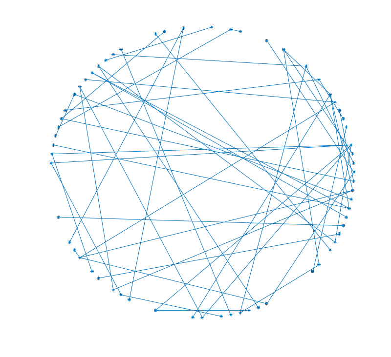
Refer to caption Refer to caption Refer to caption
(a) Graph plot. (b) Histogram of the degrees. (c) Histogram of the leverage scores.
Figure 4: Properties of an Erdős-Rényi graph. Plot (c) shows the histogram of the leverage scores, which are the optimal sampling scores when the SNR is large.

Random geometric graph. A random geometric graph is a spatial graph where each of the nodes is assigned random coordinates in the box [0,1]dsuperscript01𝑑[0,1]^{d} and an edge appears when the distance between two nodes is in a given range [58]. We used a graph lying in the box [0,1]2superscript012[0,1]^{2}, and two nodes are connected when the Euclidean distance is less than 0.030.030.03. Figure 5 illustrates some properties of the random geometric graph: Figure 5(a) shows the graph plot; Figure 5(b) shows the histogram of the degrees that concentrate around 30, as expected (this matches previous assertion that given proper parameters, the degree distribution of a random geometric graph is the same as that of an Erdős-Rényi graph [58]); Figure 5(c) shows the histogram of the leverage scores of V(20)subscriptV20\operatorname{V}_{(20)}, which are the optimal sampling scores when the SNR is large; and Figure 5(d) shows the histogram of the leverage score on a log-scale. We see that the histogram of the leverage scores is skewed; this means that a few nodes are more important than other nodes during sampling and have much higher probabilities to be chosen. In [58], the authors show that the cluster properties are different for a random geometric graph and an Erdős-Rényi graph. The proposed sampling scores capture these cluster properties through the decomposition of the graph adjacency matrix. Based on the above, a random geometric graph is approximately a Type-2 graph.
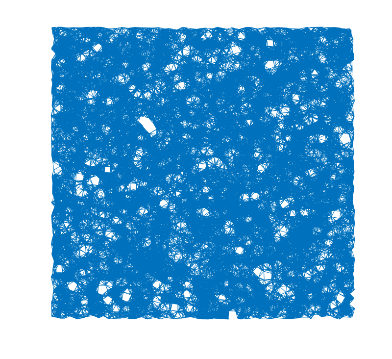
Refer to caption Refer to caption Refer to caption Refer to caption
(a) Graph plot. (b) Histogram of the degrees. (c) Histogram of the leverage scores. (d) Histogram of the leverage scores
(log-scale).
Figure 5: Properties of a random geometric graph. Plot (c) shows the histogram of the leverages score, which are the optimal sampling scores when the SNR is large. Plot (d) shows the log-scale histogram of the leverage scores, which confirms that the leverage scores approximately follow a power-law distribution.

Small-world graph. A small-world graph is a graph where most nodes are not neighbors of one another, but can be reached from any other node by a small number of hops (steps) [2, 3]. It is well known that many real-world graphs, including social networks, the connectivity of the Internet, and gene networks show small-world graph characteristics. We use a graph generated from the Watts–Strogatz model, where a ring graph is first built, followed by the rewiring of the edges with probability 0.01%percent0.010.01\%. Figure 6 illustrates some properties of the small-world graph: Figure 6(a) shows the graph plot; Figure 6(b) shows the histogram of the degrees that concentrate around 2 (a few nodes have 6 neighbors because of rewiring); Figure 6(c) shows the histogram of the leverage scores of V(20)subscriptV20\operatorname{V}_{(20)}, which are the optimal sampling scores when the SNR is large; and Figure 6(d) shows the histogram of the leverage scores on a log-scale. We see that the histogram of the leverage scores is skewed; this means that a few nodes are more important than others during sampling and have much higher probabilities to be chosen, similarly to the random geometric graph. Based on the above, a small-world graph is approximately a Type-2 graph.
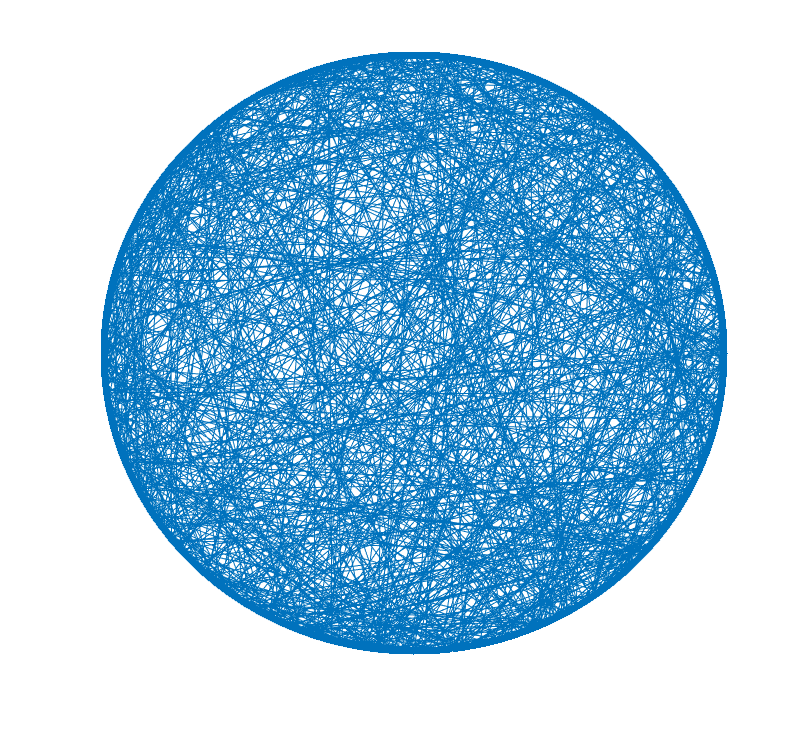
Refer to caption Refer to caption Refer to caption Refer to caption
(a) Graph plot. (b) Histogram of the degrees. (c) Histogram of the leverage scores. (d) Histogram of the leverage scores
(log-scale).
Figure 6: Properties of a small-world graph. Plot (c) shows the histogram of the leverage score, which is the optimal sampling score when the SNR is large. Plot (d) shows the log-scale histogram of the leverage scores, which confirms that the leverage scores approximately follow a power-law distribution.

Power-law graph. A power-law graph is a graph where the more connected a node is, the more likely it is to receive new links, known as a preferential attachment graph [2, 3]. It is well known that the degree distribution of a preferential attachment graph follows the power law. We use a graph generated from the Barabási-Albert model, where new nodes are added to the network one at a time. Each new node is connected to one existing node with a probability that is proportional to the number of links that the existing nodes already have. Figure 7 illustrates some properties of the small-world graph: Figure 7(a) shows the graph plot; Figure 7(b) shows the histogram of the degrees that is skewed, which clearly follows the power law; Figure 7(c) shows the histogram of the leverage scores of V(20)subscriptV20\operatorname{V}_{(20)}, which are the optimal sampling scores when the SNR is large; and Figure 7(d) shows the histogram of the leverage scores on a log-scale. We see that the histogram of the leverage scores is skewed; this means that a few nodes are more important than others during sampling and have much higher probabilities to be chosen, similarly to the random geometric graph and the small-world graph. Based on the above, a power-law graph is approximately a Type-2 graph.
Refer to caption Refer to caption Refer to caption Refer to caption
(a) Graph plot. (b) Histogram of the degrees. (c) Histogram of the leverage scores. (d) Histogram of the leverage scores
(log-scale).
Figure 7: Properties of a power-law graph. Plot (c) shows the histogram of the leverage score, which is the optimal sampling score when the SNR is large. Plot (d) shows the log-scale histogram of the leverage scores, which confirms that the leverage scores approximately follow a power-law distribution.

Types. Based on our observation of the graph Fourier transform matrices of each graph, the ring graph and the Erdős-Rényi graph approximately satisfy the requirement to be the Type-1 graph, while the random geometric graph, the small-world graph and the power-law graph approximately satisfy the requirement to be the Type-2 graph. We thus expect that the experimentally designed sampling has similar performance to uniform sampling for the ring graph and the Erdős-Rényi graph, while it outperforms uniform sampling for the random geometric graph, the small-world graph and the power-law graph.

VII-B Simulated Graph Signals

For each graph AA\operatorname{A}, we generate 1,000 graph signals through the following two steps: We first generate the graph frequency components as

x^k{𝒩(1,0.52)when k<K;=K2β/k2βwhen kK.subscript^𝑥𝑘casessimilar-toabsent𝒩1superscript0.52when 𝑘𝐾absentsuperscript𝐾2𝛽superscript𝑘2𝛽when 𝑘𝐾\displaystyle\widehat{x}_{k}\left\{\begin{array}[]{ll}\sim\mathcal{N}(1,0.5^{2})&\mbox{when }k<K;\\ ={K^{2\beta}}/{k^{2\beta}}&\mbox{when }k\geq K.\end{array}\right. (18)

We then normalize 𝐱^^𝐱\widehat{\mathbf{x}} to have unit norm, and obtain 𝐱=V𝐱^𝐱V^𝐱\mathbf{x}=\operatorname{V}\widehat{\mathbf{x}}. It is clear that 𝐱ABLA(K,β,μ)𝐱subscriptABLA𝐾𝛽𝜇\mathbf{x}\in\operatorname{ABL}_{\operatorname{A}}(K,\beta,\mu), where K=10𝐾10K=10 and β𝛽\beta varies as 0.50.50.5 and 111. During sampling, we simulate noise ϵ𝒩(0,σ2)similar-toitalic-ϵ𝒩0superscript𝜎2\epsilon\sim\mathcal{N}(0,\sigma^{2}), vary the sample size m𝑚m from 1,00010001,000 to 20,0002000020,000, and vary σ2superscript𝜎2\sigma^{2} from low noise level 104superscript10410^{-4} (𝐱2/ϵ2=100subscriptnorm𝐱2subscriptnormitalic-ϵ2100\left\|\mathbf{x}\right\|_{2}/\left\|\epsilon\right\|_{2}=100) to high noise level 0.020.020.02 (𝐱2/ϵ2=0.5subscriptnorm𝐱2subscriptnormitalic-ϵ20.5\left\|\mathbf{x}\right\|_{2}/\left\|\epsilon\right\|_{2}=0.5). During recovery, we set the bandwidth K=max(10,m1/2β+1)𝐾10superscript𝑚12𝛽1K=\max(10,m^{1/2\beta+1}) as suggested in Corollaries 4 and 6.

VII-C Results

We compare four sampling strategies, including uniform sampling (in blue), leverage score based sampling (in orange), square root of the leverage score based sampling (in purple), and degree based sampling (in red). Note that the last three sampling strategies all belong to experimentally designed sampling because they are designed based on the structure of the graph. As shown in Section V-B, leverage score based sampling is approximately optimal when the SNR is large, square root of the leverage score based sampling is approximately the optimal when the SNR is small. We also use the degrees as the sampling scores because previous works show that the largest eigenvectors of adjacency matrices often have most of their mass localized on high-degree nodes [59, 60], which implies the high correlation between degree and leverage score. We evaluate the recovery performance by using the MSE,

MSE=𝐱𝐱22,MSEsuperscriptsubscriptnormsuperscript𝐱𝐱22\displaystyle{\rm MSE}\ =\ \left\|\mathbf{x}^{*}-\mathbf{x}\right\|_{2}^{2},

where 𝐱superscript𝐱\mathbf{x}^{*} is the recovered graph signal and 𝐱𝐱\mathbf{x} is the original graph signal. The simulation results for the ring graph, the Erdős-Rényi graph, the random geometric graph, the small-world graph and the power-law graph are shown in Figures 891011 and 12, respectively. We summarize the important points below.

  • All of the sampling strategies perform similarly on the ring graph and the Erdős-Rényi graph, matching Corollary 4.

  • Experimentally designed sampling outperforms uniform sampling on the random geometric graph, the small-world graph and the power-law graph, matching Corollary 6. Especially for the small-world graph and the power-law graph, uniform sampling is much worse than experimentally designed sampling.

  • Leverage score based sampling outperforms all other sampling strategies when the noise level is low.

  • Square root of the leverage score based sampling outperforms all other sampling strategies when the noise level is high.

  • Degree based sampling outperforms uniform sampling because of its correlation to the leverage score based sampling, but for the small-world graph, degree based sampling is still much worse than leverage score based sampling.

  • When β𝛽\beta is larger, the recovery performance is better because less energy is concentrated in the high-frequency band for approximately bandlimited graph signals.

  • When σ2superscript𝜎2\sigma^{2} is smaller, the recovery performance is better because of less noise.

  • The degree distribution is not a reliable indicator of when experimentally designed sampling outperforms uniform sampling. The degree distributions of the Erdős-Rényi graph and the random geometric graph are similar, but experimentally designed sampling only outperforms uniform sampling on the random geometric graph. This implies that the first-order information provided by the degree is not sufficient in designing samples.

Refer to caption Refer to caption
(a) β=0.5,σ2=104formulae-sequence𝛽0.5superscript𝜎2superscript104\beta=0.5,\sigma^{2}=10^{-4} (b) β=1,σ2=104formulae-sequence𝛽1superscript𝜎2superscript104\beta=1,\sigma^{2}=10^{-4}
Refer to caption Refer to caption
(d) β=0.5,σ2=2×10²formulae-sequence𝛽0.5superscript𝜎22superscript102\beta=0.5,\sigma^{2}=2\times 10^{-2} (e) β=1,σ2=2×10²formulae-sequence𝛽1superscript𝜎22superscript102\beta=1,\sigma^{2}=2\times 10^{-2}
Figure 8: MSE comparison for the ring graph for uniform sampling (in blue), leverage score based sampling (in orange), square root of the leverage score based sampling (in purple) and degree based sampling (in red).
Refer to caption Refer to caption
(a) β=0.5,σ2=104formulae-sequence𝛽0.5superscript𝜎2superscript104\beta=0.5,\sigma^{2}=10^{-4}. (b) β=1,σ2=104formulae-sequence𝛽1superscript𝜎2superscript104\beta=1,\sigma^{2}=10^{-4}.
Refer to caption Refer to caption
(c) β=0.5,σ2=2×10²formulae-sequence𝛽0.5superscript𝜎22superscript102\beta=0.5,\sigma^{2}=2\times 10^{-2}. (d) β=1,σ2=2×10²formulae-sequence𝛽1superscript𝜎22superscript102\beta=1,\sigma^{2}=2\times 10^{-2}.
Figure 9: MSE comparison for the Erdős-Rényi graph for uniform sampling (in blue), leverage score based sampling (in orange), square root of the leverage score based sampling (in purple) and degree based sampling (in red).
Refer to caption Refer to caption
(a) β=0.5,σ2=104formulae-sequence𝛽0.5superscript𝜎2superscript104\beta=0.5,\sigma^{2}=10^{-4}. (b) β=1,σ2=104formulae-sequence𝛽1superscript𝜎2superscript104\beta=1,\sigma^{2}=10^{-4}.
Refer to caption Refer to caption
(c) β=0.5,σ2=2×10²formulae-sequence𝛽0.5superscript𝜎22superscript102\beta=0.5,\sigma^{2}=2\times 10^{-2}. (d) β=1,σ2=2×10²formulae-sequence𝛽1superscript𝜎22superscript102\beta=1,\sigma^{2}=2\times 10^{-2}.
Figure 10: MSE comparison for the random geometric graph for uniform sampling (in blue), leverage score based sampling (in orange), square root of the leverage score based sampling (in purple) and degree based sampling (in red).
Refer to caption Refer to caption
(a) β=0.5,σ2=104formulae-sequence𝛽0.5superscript𝜎2superscript104\beta=0.5,\sigma^{2}=10^{-4}. (b) β=1,σ2=104formulae-sequence𝛽1superscript𝜎2superscript104\beta=1,\sigma^{2}=10^{-4}.
Refer to caption Refer to caption
(c) β=0.5,σ2=2×10²formulae-sequence𝛽0.5superscript𝜎22superscript102\beta=0.5,\sigma^{2}=2\times 10^{-2}. (d) β=1,σ2=2×10²formulae-sequence𝛽1superscript𝜎22superscript102\beta=1,\sigma^{2}=2\times 10^{-2}.
Figure 11: MSE comparison for the small-world graph for uniform sampling (in blue), leverage score based sampling (in orange), square root of the leverage score based sampling (in purple) and degree based sampling (in red).
Refer to caption Refer to caption
(a) β=0.5,σ2=104formulae-sequence𝛽0.5superscript𝜎2superscript104\beta=0.5,\sigma^{2}=10^{-4}. (b) β=1,σ2=104formulae-sequence𝛽1superscript𝜎2superscript104\beta=1,\sigma^{2}=10^{-4}.
Refer to caption Refer to caption
(c) β=0.5,σ2=2×10²formulae-sequence𝛽0.5superscript𝜎22superscript102\beta=0.5,\sigma^{2}=2\times 10^{-2}. (d) β=1,σ2=2×10²formulae-sequence𝛽1superscript𝜎22superscript102\beta=1,\sigma^{2}=2\times 10^{-2}.
Figure 12: MSE comparison for the power-law graph for uniform sampling (in blue), leverage score based sampling (in orange), square root of the leverage score based sampling (in purple) and degree based sampling (in red).

VII-D Discussion

Graph Fourier basis is critical for understanding the graph structure. For example, given the graph Fourier basis, Theorem 3 shows that active sampling does not fundamentally outperform experimentally designed sampling while Corollary 6 shows that experimentally designed sampling fundamentally outperforms uniform sampling on type-2 graphs. In other words, graph Fourier basis is critical for choosing samples.

For irregular (Type-2) graphs, using experimentally designed sampling to choose anchor points can fundamentally aid semi-supervised learning (not true for regular, Type-1 graphs), a technique for training classifiers with both labeled and unlabeled data. Semi-supervised learning assumes that unlabeled data can provide distribution information to build a stronger classifier [61]. Many algorithms for semi-supervised learning are based on graphs that are constructed from a given dataset [61], often by modeling each node as a data sample and connecting two nodes by an edge if the distance between their features is in a given range, which is similar to the construction of random geometric graphs. Based on the assumption that adjacent nodes have similar labels, semi-supervised learning diffuses label probabilities from labeled data to unlabeled data along the graph structure and classifies unlabeled data according to those label probabilities. While in some works [62, 63], training data is selected uniformly and randomly, in others, algorithms are designed adapted to the structure [64, 65], which is essentially equivalent to experimentally designed sampling we propose. In other words, experimentally designed sampling is used implicitly without being able to articulate when and why it works; this paper, on the other hand, provides a comprehensive explanation of why experimentally designed sampling helps semi-supervised learning through showing the lower and upper bounds of three sampling strategies.

VIII Conclusions

We build a theoretical foundation for the recovery of a newly proposed class of smooth graph signals, approximately bandlimited signals, which generalizes the class of bandlimited graph signals, under uniform sampling, experimentally designed sampling and active sampling. We show that experimentally designed sampling and active sampling have the same fundamental limitations, and can outperform uniform sampling on irregular graphs. We propose a recovery strategy and analyze its statistical properties. We show that the proposed recovery strategy attains the optimal rates of convergence on two specific types of graphs. To validate the recovery strategy, we test it on five specific types of graphs: a ring graph with k𝑘k nearest neighbors, an Erdős-Rényi graph, a random geometric graph, a small-world graph and a power-law graph, and show that experimental results match the proposed theory well. This work also gives a comprehensive explanation for why experimentally designed sampling works for semi-supervised learning with graphs and shows the critical role of the graph Fourier basis in analyzing graph structures.

IX Acknowledgment

We gratefully acknowledge support from the NSF through awards 1130616,1421919, the University Transportation Center grant (DTRT12-GUTC11) from the US Department of Transportation, and the CMU Carnegie Institute of Technology Infrastructure Award. We also thank the editor and the reviewers for comments that led to improvements in the manuscript. Initial parts of this work were presented at SampTA 2015 [1].

References

  • [1] S. Chen, R. Varma, A. Singh, and J. Kovačević, “Signal recovery on graphs: Random versus experimentally designed sampling,” in Proc. Sampling Theory Appl., Washington, DC, May 2015, pp. 337–341.
  • [2] M. Jackson, Social and Economic Networks, Princeton University Press, 2008.
  • [3] M. Newman, Networks: An Introduction, Oxford University Press, 2010.
  • [4] D. I. Shuman, S. K. Narang, P. Frossard, A. Ortega, and P. Vandergheynst, “The emerging field of signal processing on graphs: Extending high-dimensional data analysis to networks and other irregular domains,” IEEE Signal Process. Mag., vol. 30, pp. 83–98, May 2013.
  • [5] A. Sandryhaila and J. M. F. Moura, “Big data processing with signal processing on graphs,” IEEE Signal Process. Mag., vol. 31, no. 5, pp. 80–90, Sept. 2014.
  • [6] S. Chen, R. Varma, A. Sandryhaila, and J. Kovačević, “Discrete signal processing on graphs: Sampling theory,” IEEE Trans. Signal Process., vol. 63, no. 24, pp. 6510–6523, Dec. 2015.
  • [7] A. Anis, A. Gadde, and A. Ortega, “Efficient sampling set selection for bandlimited graph signals using graph spectral proxies,” IEEE Trans. Signal Process., 2015, Submitted.
  • [8] X. Wang, P. Liu, and Y. Gu, “Local-set-based graph signal reconstruction,” IEEE Trans. Signal Process., vol. 63, no. 9, May 2015.
  • [9] S. Chen, A. Sandryhaila, J. M. F. Moura, and J. Kovačević, “Signal recovery on graphs: Variation minimization,” IEEE Trans. Signal Process., vol. 63, no. 17, pp. 4609–4624, Sept. 2015.
  • [10] S. K. Narang, Akshay Gadde, and Antonio Ortega, “Signal processing techniques for interpolation in graph structured data,” in Proc. IEEE Int. Conf. Acoust., Speech, Signal Process., Vancouver, May 2013, pp. 5445–5449.
  • [11] X. Zhu and M. Rabbat, “Approximating signals supported on graphs,” in Proc. IEEE Int. Conf. Acoust., Speech, Signal Process., Kyoto, Mar. 2012, pp. 3921–3924.
  • [12] S. Chen, T. Li, R. Varma, A. Singh, and J. Kovačević, “Signal representations on graphs: Tools and applications,” IEEE Trans. Signal Process., Mar. 2016, Submitted.
  • [13] A. Agaskar and Y. M. Lu, “A spectral graph uncertainty principle,” IEEE Trans. Inf. Theory, vol. 59, no. 7, pp. 4338–4356, July 2013.
  • [14] M. Tsitsvero, S. Barbarossa, and P. D. Lorenzo, “Signals on graphs: Uncertainty principle and sampling,” arXiv:1507.08822, 2015.
  • [15] D. Thanou, D. I. Shuman, and P. Frossard, “Learning parametric dictionaries for signals on graphs,” IEEE Trans. Signal Process., vol. 62, pp. 3849–3862, June 2014.
  • [16] S. Chen, F. Cerda, P. Rizzo, J. Bielak, J. H. Garrett, and J. Kovačević, “Semi-supervised multiresolution classification using adaptive graph filtering with application to indirect bridge structural health monitoring,” IEEE Trans. Signal Process., vol. 62, no. 11, pp. 2879–2893, June 2014.
  • [17] V. N. Ekambaram, B. Ayazifar G. Fanti, and K. Ramchandran, “Wavelet-regularized graph semi-supervised learning,” in Proc. IEEE Glob. Conf. Signal Information Process., Austin, TX, Dec. 2013, pp. 423–426.
  • [18] S. K. Narang and A. Ortega, “Perfect reconstruction two-channel wavelet filter banks for graph structured data,” IEEE Trans. Signal Process., vol. 60, pp. 2786–2799, June 2012.
  • [19] S. Chen, A. Sandryhaila, J. M. F. Moura, and J. Kovačević, “Signal denoising on graphs via graph filtering,” in Proc. IEEE Glob. Conf. Signal Information Process., Atlanta, GA, Dec. 2014, pp. 872–876.
  • [20] N. Tremblay and P. Borgnat, “Graph wavelets for multiscale community mining,” IEEE Trans. Signal Process., vol. 62, pp. 5227–5239, Oct. 2014.
  • [21] X. Dong, P. Frossard, P. Vandergheynst, and N. Nefedov, “Clustering on multi-layer graphs via subspace analysis on Grassmann manifolds,” IEEE Trans. Signal Process., vol. 62, no. 4, pp. 905–918, Feb. 2014.
  • [22] P.-Y. Chen and A.O. Hero, “Local Fiedler vector centrality for detection of deep and overlapping communities in networks,” in Proc. IEEE Int. Conf. Acoust., Speech, Signal Process., Florence, 2014, pp. 1120–1124.
  • [23] S. K. Narang and Antonio Ortega, “Compact support biorthogonal wavelet filterbanks for arbitrary undirected graphs,” IEEE Trans. Signal Process., vol. 61, no. 19, pp. 4673–4685, Oct. 2013.
  • [24] N. Tremblay and P. Borgnat, “Subgraph-based filterbanks for graph signals,” IEEE Trans. Signal Process., vol. 64, pp. 3827–3840, Mar. 2016.
  • [25] A. Sandryhaila and J. M. F. Moura, “Discrete signal processing on graphs,” IEEE Trans. Signal Process., vol. 61, no. 7, pp. 1644–1656, Apr. 2013.
  • [26] D. K. Hammond, P. Vandergheynst, and R. Gribonval, “Wavelets on graphs via spectral graph theory,” Appl. Comput. Harmon. Anal., vol. 30, pp. 129–150, Mar. 2011.
  • [27] S.l K. Narang, G. Shen, and A. Ortega, “Unidirectional graph-based wavelet transforms for efficient data gathering in sensor networks,” in Proc. IEEE Int. Conf. Acoust., Speech, Signal Process., Dallas, TX, Mar. 2010, pp. 2902–2905.
  • [28] D. I. Shuman, M. J. Faraji, , and P. Vandergheynst, “A multiscale pyramid transform for graph signals,” IEEE Trans. Signal Process., vol. 64, pp. 2119–2134, Apr. 2016.
  • [29] M. Vetterli, J. Kovačević, and V. K. Goyal, Foundations of Signal Processing, Cambridge University Press, Cambridge, 2014, http://foundationsofsignalprocessing.org.
  • [30] J. Kovačević and M. Püschel, “Algebraic signal processing theory: Sampling for infinite and finite 1-D space,” IEEE Trans. Signal Process., vol. 58, no. 1, pp. 242–257, Jan. 2010.
  • [31] M. Vetterli, P. Marziliano, and T. Blu, “Sampling signals with finite rate of innovation,” IEEE Trans. Signal Process., vol. 50, no. 6, pp. 1417–1428, June 2002.
  • [32] P. L. Dragotti, M. Vetterli, and T. Blu, “Sampling moments and reconstructing signals of finite rate of innovation: Shannon meets Strang-Fix,” IEEE Trans. Signal Process., vol. 55, 2007.
  • [33] E. J. Candés, J. K. Romberg, and T. Tao, “Stable signal recovery from incomplete and inaccurate measurements,” Commun. Pure Appl. Math., vol. 59, pp. 1207–1223, Aug. 2006.
  • [34] E. J. Candès, Y. Eldar, D. Needell, and P. Randall, “Compressed sensing with coherent and redundant dictionaries,” Appl. Comput. Harmon. Anal., vol. 31, pp. 59–73, 2010.
  • [35] Y. M. Lu and M. N. Do, “Sampling signals from a union of subspaces,” IEEE Signal Process. Mag., vol. 25, no. 2, pp. 41–47, Mar. 2008.
  • [36] T. Blumensath and M. E. Davies, “Sampling theorems for signals from the union of finite-dimensional linear subspaces,” IEEE Trans. Inf. Theory, vol. 55, pp. 1872–1882, Apr. 2009.
  • [37] I. Z. Pesenson, “Sampling in Paley-Wiener spaces on combinatorial graphs,” Trans. Am. Math. Soc., vol. 360, no. 10, pp. 5603–5627, May 2008.
  • [38] X. Zhu and M. Rabbat, “Graph spectral compressed sensing for sensor networks,” in Proc. IEEE Int. Conf. Acoust., Speech, Signal Process., Kyoto, Mar. 2012, pp. 2865–2868.
  • [39] A. Anis, A. Gadde, and A. Ortega, “Towards a sampling theorem for signals on arbitrary graphs,” in Proc. IEEE Int. Conf. Acoust., Speech, Signal Process., Florence, May 2014, pp. 3864–3868.
  • [40] S. Chen, A. Sandryhaila, and J. Kovačević, “Sampling theory for graph signals,” in Proc. IEEE Int. Conf. Acoust., Speech, Signal Process., Brisbane, Apr. 2015, pp. 3392–3396.
  • [41] X. Wang, M. Wang, and Y. Gu, “A distributed tracking algorithm for reconstruction of graph signals,” IEEE J. Sel. Topics Signal Process., vol. 9, no. 4, June 2015.
  • [42] S. Chen, A. Sandryhaila, and J. Kovačević, “Distributed algorithm for graph signal inpainting,” in Proc. IEEE Int. Conf. Acoust., Speech, Signal Process., Brisbane, Apr. 2015, pp. 3731–3735.
  • [43] X. Wang, J. Chen, and Y. Gu, “Local measurement and reconstruction for noisy graph signals,” arXiv:1504.01456, 2015.
  • [44] A. G. Marques, S. Segarra, G. Leus, and A. Ribeiro, “Sampling of graph signals with successive local aggregations,” arXiv:1504.04687, 2015.
  • [45] S. Segarra, A. G. Marques, G. Leus, and A. Ribeiro, “Reconstruction of graph signals through percolation from seeding nodes,” IEEE Trans. Signal Process., 2015, Submitted.
  • [46] R. Castro, R. Willett, and R. Nowak, “Faster rates in regression via active learning,” in Proc. Neural Information Process. Syst., Vancouver, Dec. 2005.
  • [47] R. Castro and R. Nowak, “Minimax bounds for active learning,” IEEE Trans. Inf. Theory, vol. 54, no. 5, pp. 2339–2353, July 2008.
  • [48] A. P. Korostelev and A. B. Tsybakov, Minimax theory of image reconstruction, Lecture Notes in Stat. Springer, 1993.
  • [49] A. Sandryhaila and J. M. F. Moura, “Discrete signal processing on graphs: Frequency analysis,” IEEE Trans. Signal Process., vol. 62, no. 12, pp. 3042–3054, June 2014.
  • [50] J. Sharpnack and A. Singh, “Identifying graph-structured activation patterns in networks,” in Proc. Neural Information Process. Syst., Vancouver, Dec. 2010, pp. 2137–2145.
  • [51] I. M. Johnstone, Minimax Bayes, Asymptotic Minimax and Sparse Wavelet Priors, Statistical Decision Theory and Related Topics V. Springer, 1994.
  • [52] T. Ji, S. Chen, R. Varma, and J. Kovačević, “Energy-efficient route planning of autonomous vehicles based on graph signal recovery,” in Proc. Allerton Conf. on Commun., Control and Comput., Allerton, IL, Oct. 2015.
  • [53] A. Sakiyama, Y. Tanaka, T. Tanaka, and A. Ortega, “Efficient sensor position selection using graph signal sampling theory,” in Proc. IEEE Int. Conf. Acoust., Speech, Signal Process., Shanghai, Mar. 2016, pp. 6225–6229.
  • [54] N. Tremblay, G. Puy, R. Gribonval, and P. Vandergheynst, “Compressive spectral clustering,” arXiv:1602.02018, 2016.
  • [55] A. P. Korostelev and A. B. Tsybakov, Minimax Theory of Image Reconstruction, Lecture Notes in Stat. Springer, 1993.
  • [56] P. Ma, M. W. Mahoney, and B. Yu, “A statistical perspective on algorithmic leveraging,” J. Mach. Learn. Res., vol. 16, pp. 861–911, 2015.
  • [57] A. Sandryhaila, J. Kovačević, and M. Püschel, “Algebraic signal processing theory: 1-D nearest-neighbor models,” IEEE Trans. Signal Process., vol. 60, no. 5, pp. 2247–2259, May 2012.
  • [58] J. Dall and M. Christensen, “Random geometric graphs,” Phys. Rev. E, vol. 66, July 2002.
  • [59] K. I. Goh, B. Kahng, and D. Kim, “Spectra and eigenvectors of scale-free networks,” Phys Rev E, vol. 64, no. 5, Nov. 2001.
  • [60] M. Cucuringu and M. W. Mahoney, “Localization on low-order eigenvectors of data matrices,” Technical Report, Preprint: arXiv:1109.1355, 2011.
  • [61] X. Zhu, “Semi-supervised learning literature survey,” Tech. Rep. 1530, University Wisconsin-Madison, 2005.
  • [62] X. Zhu, J. Lafferty, and Z. Ghahramani, “Combining active learning and semi-supervised learning using Gaussian fields and harmonic functions,” in Proc. Int. Conf. Mach. Learn. Workshop on Continuum from Labeled to Unlabeled Data in Mach. Learn. Data Mining, Washington, DC, 2003, pp. 58–65.
  • [63] M. Belkin and P. Niyogi, “Laplacian eigenmaps for dimensionality reduction and data representation,” Neur. Comput., vol. 13, pp. 1373–1396, 2003.
  • [64] Q. Gu and J. Han, “Towards active learning on graphs: An error bound minimization approach,” in Proc. IEEE Int. Conf. Data Mining, Brussels, Dec. 2012, pp. 882–887.
  • [65] A. Gadde, A. Anis, and A. Ortega, “Active semi-supervised learning using sampling theory for graph signals,” in Proc. ACM Int. Conf. Knowl. Discovery Data Mining, New York, NY, 2014, pp. 492–501.

Appendix A Appendices

A-A Proof of Theorem 3

We aim to construct a typical set of vectors in \mathcal{F}, and use the Fano’s method. Let 𝐯ksubscript𝐯𝑘\mathbf{v}_{k} be the k𝑘kth column of VV\operatorname{V}, 𝐯(i)superscript𝐯𝑖\mathbf{v}^{(i)} be the i𝑖ith row of VV\operatorname{V}, 𝒳𝒳\mathcal{X} be a pruned hypercube and

={𝐱(𝐰)=V𝐱^𝐰=k=κ02κ01wkψk,𝐰𝒳},\mathcal{F}^{\prime}=\{\mathbf{x}^{(\mathbf{w})}=\operatorname{V}\widehat{\mathbf{x}}\odot\mathbf{w}=\sum_{k=\kappa_{0}}^{2\kappa_{0}-1}w_{k}\psi_{k},~{}~{}\mathbf{w}\in\mathcal{X}\},

where κ0subscript𝜅0\kappa_{0} is no smaller than the bandwidth K𝐾K,

ψk=x^k𝐯k=(±)kcμ𝐱22κ0(1+k2β)𝐯k,subscript𝜓𝑘subscript^𝑥𝑘subscript𝐯𝑘superscriptplus-or-minus𝑘𝑐𝜇superscriptsubscriptnorm𝐱22subscript𝜅01superscript𝑘2𝛽subscript𝐯𝑘\psi_{k}=\widehat{x}_{k}\mathbf{v}_{k}=(\pm)^{k}\sqrt{\frac{c\mu\left\|\mathbf{x}\right\|_{2}^{2}}{\kappa_{0}(1+k^{2\beta})}}\mathbf{v}_{k},

and 0<c<10𝑐10<c<1. It is easy to check that superscript\mathcal{F}^{\prime}\subseteq\mathcal{F}. Let d(𝐱,𝐲)=𝐱𝐲2𝑑𝐱𝐲subscriptnorm𝐱𝐲2d(\mathbf{x},\mathbf{y})=\left\|\mathbf{x}-\mathbf{y}\right\|_{2}; we thus have

d2(𝐱(𝐰),𝐱(𝐮))superscript𝑑2superscript𝐱𝐰superscript𝐱𝐮\displaystyle d^{2}(\mathbf{x}^{(\mathbf{w})},\mathbf{x}^{(\mathbf{u})}) =\displaystyle= V𝐱^(𝐰𝐮)222superscriptsubscriptnormdirect-productV^𝐱superscript𝐰𝐮222\displaystyle\left\|\operatorname{V}\widehat{\mathbf{x}}\odot(\mathbf{w}-\mathbf{u})^{2}\right\|_{2}^{2}
=\displaystyle= k=κ02κ01(wkuk)2x^k2superscriptsubscript𝑘subscript𝜅02subscript𝜅01superscriptsubscript𝑤𝑘subscript𝑢𝑘2superscriptsubscript^𝑥𝑘2\displaystyle\sum_{k=\kappa_{0}}^{2\kappa_{0}-1}(w_{k}-u_{k})^{2}\widehat{x}_{k}^{2}
=\displaystyle= k=κ02κ01(wkuk)2cμ𝐱22κ0(1+k2β)superscriptsubscript𝑘subscript𝜅02subscript𝜅01superscriptsubscript𝑤𝑘subscript𝑢𝑘2𝑐𝜇superscriptsubscriptnorm𝐱22subscript𝜅01superscript𝑘2𝛽\displaystyle\sum_{k=\kappa_{0}}^{2\kappa_{0}-1}(w_{k}-u_{k})^{2}\frac{c\mu\left\|\mathbf{x}\right\|_{2}^{2}}{\kappa_{0}(1+k^{2\beta})}
(a)superscript𝑎\displaystyle\stackrel{{\scriptstyle(a)}}{{\geq}} k=κ02κ01(wkuk)2cμ𝐱22κ0(1+(2κ0)2β)superscriptsubscript𝑘subscript𝜅02subscript𝜅01superscriptsubscript𝑤𝑘subscript𝑢𝑘2𝑐𝜇superscriptsubscriptnorm𝐱22subscript𝜅01superscript2subscript𝜅02𝛽\displaystyle\sum_{k=\kappa_{0}}^{2\kappa_{0}-1}(w_{k}-u_{k})^{2}\cdot\frac{c\mu\left\|\mathbf{x}\right\|_{2}^{2}}{\kappa_{0}(1+(2\kappa_{0})^{2\beta})}
(b)superscript𝑏\displaystyle\stackrel{{\scriptstyle(b)}}{{\geq}} κ08cμ𝐱22κ0(1+(2κ0)2β)c1μκ02β𝐱22,subscript𝜅08𝑐𝜇superscriptsubscriptnorm𝐱22subscript𝜅01superscript2subscript𝜅02𝛽subscript𝑐1𝜇superscriptsubscript𝜅02𝛽superscriptsubscriptnorm𝐱22\displaystyle\frac{\kappa_{0}}{8}\cdot\frac{c\mu\left\|\mathbf{x}\right\|_{2}^{2}}{\kappa_{0}(1+(2\kappa_{0})^{2\beta})}\ \geq\ c_{1}\mu\kappa_{0}^{-2\beta}\left\|\mathbf{x}\right\|_{2}^{2},

where (a)𝑎(a) follows from k2K𝑘2𝐾k\leq 2K, and (b)𝑏(b) from the Varshamov-Gilbert lemma. To use the Fanno’s method, we need to bound the Kullback-Leibler divergence,

KL(p𝐰,p𝐰0|)𝐾𝐿subscript𝑝𝐰conditionalsubscript𝑝subscript𝐰0\displaystyle KL(p_{\mathbf{w}},p_{\mathbf{w}_{0}}|\mathcal{M})
=\displaystyle= i𝔼𝐰[logp(yixi(𝐰))p(yixi(𝐰0))]subscript𝑖subscript𝔼𝐰delimited-[]𝑝subscript𝑦𝑖subscriptsuperscript𝑥𝐰𝑖𝑝subscript𝑦𝑖subscriptsuperscript𝑥subscript𝐰0𝑖\displaystyle\sum_{i\in\mathcal{M}}\mathbb{E}_{\mathbf{w}}\left[\log\frac{p(y_{i}-x^{(\mathbf{w})}_{i})}{p(y_{i}-x^{(\mathbf{w}_{0})}_{i})}\right]
\displaystyle\leq i[12σ2(xi(𝐰)xi(𝐰0))2]subscript𝑖delimited-[]12superscript𝜎2superscriptsubscriptsuperscript𝑥𝐰𝑖subscriptsuperscript𝑥subscript𝐰0𝑖2\displaystyle\sum_{i\in\mathcal{M}}\left[\frac{1}{2\sigma^{2}}(x^{(\mathbf{w})}_{i}-x^{(\mathbf{w}_{0})}_{i})^{2}\right]
=\displaystyle= i[12σ2(𝐯(i)(𝐱^𝐰))2]subscript𝑖delimited-[]12superscript𝜎2superscriptsuperscriptsuperscript𝐯𝑖direct-product^𝐱𝐰2\displaystyle\sum_{i\in\mathcal{M}}\left[\frac{1}{2\sigma^{2}}\left({\mathbf{v}^{(i)}}^{*}(\widehat{\mathbf{x}}\odot\mathbf{w})\right)^{2}\right]
=\displaystyle= 12σ2i(k=κ02κ01x^kwkVik)212superscript𝜎2subscript𝑖superscriptsuperscriptsubscript𝑘subscript𝜅02subscript𝜅01subscript^𝑥𝑘subscript𝑤𝑘subscriptV𝑖𝑘2\displaystyle\frac{1}{2\sigma^{2}}\sum_{i\in\mathcal{M}}\left(\sum_{k=\kappa_{0}}^{2\kappa_{0}-1}\widehat{x}_{k}w_{k}\operatorname{V}_{ik}\right)^{2}
=\displaystyle= 12σ2i(k=κ02κ01(x^kwkVik)2\displaystyle\frac{1}{2\sigma^{2}}\sum_{i\in\mathcal{M}}\bigg{(}\sum_{k=\kappa_{0}}^{2\kappa_{0}-1}\left(\widehat{x}_{k}w_{k}\operatorname{V}_{ik}\right)^{2}
+k,k=κ0,kk2κ01x^kx^kwkwkVikVik)\displaystyle+\sum_{k,k^{\prime}=\kappa_{0},k\neq k^{\prime}}^{2\kappa_{0}-1}\widehat{x}_{k}\widehat{x}_{k^{\prime}}w_{k}w_{k^{\prime}}\operatorname{V}_{ik}\operatorname{V}_{ik^{\prime}}\bigg{)}
\displaystyle\leq 12σ2i(k=κ02κ01cμ𝐱22wk2Vik22κ0(1+k2β)\displaystyle\frac{1}{2\sigma^{2}}\sum_{i\in\mathcal{M}}\bigg{(}\sum_{k=\kappa_{0}}^{2\kappa_{0}-1}\frac{c\mu\left\|\mathbf{x}\right\|_{2}^{2}w_{k}^{2}\operatorname{V}_{ik}^{2}}{2\kappa_{0}(1+k^{2\beta})}
+k,k=κ0,kk2κ01(1)k+kcμ𝐱22wkwkVikVikκ01+k2β1+k2β)\displaystyle+\sum_{k,k^{\prime}=\kappa_{0},k\neq k^{\prime}}^{2\kappa_{0}-1}(-1)^{k+k^{\prime}}\frac{c\mu\left\|\mathbf{x}\right\|_{2}^{2}w_{k}w_{k^{\prime}}\operatorname{V}_{ik}\operatorname{V}_{ik^{\prime}}}{\kappa_{0}\sqrt{1+k^{2\beta}}\sqrt{1+k^{\prime 2\beta}}}\bigg{)}
\displaystyle\leq cμ𝐱22σ2ik=κ02κ01Vik2κ0(1+κ02β)+δsuperscript𝑐𝜇superscriptsubscriptnorm𝐱22superscript𝜎2subscript𝑖superscriptsubscript𝑘subscript𝜅02subscript𝜅01superscriptsubscriptV𝑖𝑘2subscript𝜅01superscriptsubscript𝜅02𝛽𝛿\displaystyle\frac{c^{\prime}\mu\left\|\mathbf{x}\right\|_{2}^{2}}{\sigma^{2}}\sum_{i\in\mathcal{M}}\sum_{k=\kappa_{0}}^{2\kappa_{0}-1}\frac{\operatorname{V}_{ik}^{2}}{\kappa_{0}(1+\kappa_{0}^{2\beta})}+\delta
asymptotically-equals\displaystyle\asymp cμ𝐱22σ2κ0(2β+1)ik=κ02κ01Vik2,superscript𝑐𝜇superscriptsubscriptnorm𝐱22superscript𝜎2superscriptsubscript𝜅02𝛽1subscript𝑖superscriptsubscript𝑘subscript𝜅02subscript𝜅01superscriptsubscriptV𝑖𝑘2\displaystyle\frac{c^{\prime}\mu\left\|\mathbf{x}\right\|_{2}^{2}}{\sigma^{2}}\kappa_{0}^{-(2\beta+1)}\sum_{i\in\mathcal{M}}\sum_{k=\kappa_{0}}^{2\kappa_{0}-1}\operatorname{V}_{ik}^{2},

where δ=k,k=κ0,kk2κ01(1)k+kcμ𝐱22wkwkVikVikκ01+k2β1+k2β𝛿superscriptsubscriptformulae-sequence𝑘superscript𝑘subscript𝜅0𝑘superscript𝑘2subscript𝜅01superscript1𝑘superscript𝑘𝑐𝜇superscriptsubscriptnorm𝐱22subscript𝑤𝑘subscript𝑤superscript𝑘subscriptV𝑖𝑘subscriptV𝑖superscript𝑘subscript𝜅01superscript𝑘2𝛽1superscript𝑘2𝛽\delta=\sum_{k,k^{\prime}=\kappa_{0},k\neq k^{\prime}}^{2\kappa_{0}-1}(-1)^{k+k^{\prime}}\frac{c\mu\left\|\mathbf{x}\right\|_{2}^{2}w_{k}w_{k^{\prime}}\operatorname{V}_{ik}\operatorname{V}_{ik^{\prime}}}{\kappa_{0}\sqrt{1+k^{2\beta}}\sqrt{1+k^{\prime 2\beta}}} is small because of the cross signs. For uniform sampling, the sampling set \mathcal{M} is chosen randomly, thus, we have

KL(p𝐰,p𝐰0)𝐾𝐿subscript𝑝𝐰subscript𝑝subscript𝐰0\displaystyle KL(p_{\mathbf{w}},p_{\mathbf{w}_{0}})
=\displaystyle= 𝔼[KL(p𝐰,p𝐰0|)]subscript𝔼delimited-[]𝐾𝐿subscript𝑝𝐰conditionalsubscript𝑝subscript𝐰0\displaystyle\mathbb{E}_{\mathcal{M}}\left[KL(p_{\mathbf{w}},p_{\mathbf{w}_{0}}|\mathcal{M})\right]
\displaystyle\leq cμ𝐱22σ2κ0(2β+1)𝔼(ik=κ02κ01Vik2)𝑐𝜇superscriptsubscriptnorm𝐱22superscript𝜎2superscriptsubscript𝜅02𝛽1subscript𝔼subscript𝑖superscriptsubscript𝑘subscript𝜅02subscript𝜅01superscriptsubscriptV𝑖𝑘2\displaystyle\frac{c\mu\left\|\mathbf{x}\right\|_{2}^{2}}{\sigma^{2}}\kappa_{0}^{-(2\beta+1)}\mathbb{E}_{\mathcal{M}}\left(\sum_{i\in\mathcal{M}}\sum_{k=\kappa_{0}}^{2\kappa_{0}-1}\operatorname{V}_{ik}^{2}\right)
=(a)superscript𝑎\displaystyle\stackrel{{\scriptstyle(a)}}{{=}} cμ𝐱22σ2K(2β+1)𝔼i(mk=κ02κ01Vik2)𝑐𝜇superscriptsubscriptnorm𝐱22superscript𝜎2superscript𝐾2𝛽1subscript𝔼𝑖𝑚superscriptsubscript𝑘subscript𝜅02subscript𝜅01superscriptsubscriptV𝑖𝑘2\displaystyle\frac{c\mu\left\|\mathbf{x}\right\|_{2}^{2}}{\sigma^{2}}K^{-(2\beta+1)}\mathbb{E}_{i}\left(m\sum_{k=\kappa_{0}}^{2\kappa_{0}-1}\operatorname{V}_{ik}^{2}\right)
=\displaystyle= cμ𝐱22σ2K(2β+1)mj=1Nk=κ02κ01Vjk2(j=i)𝑐𝜇superscriptsubscriptnorm𝐱22superscript𝜎2superscript𝐾2𝛽1𝑚superscriptsubscript𝑗1𝑁superscriptsubscript𝑘subscript𝜅02subscript𝜅01superscriptsubscriptV𝑗𝑘2𝑗𝑖\displaystyle\frac{c\mu\left\|\mathbf{x}\right\|_{2}^{2}}{\sigma^{2}}K^{-(2\beta+1)}m\sum_{j=1}^{N}\sum_{k=\kappa_{0}}^{2\kappa_{0}-1}\operatorname{V}_{jk}^{2}\mathbb{P}(j=i)
=\displaystyle= cμ𝐱22σ2κ0(2β+1)mNj=1Nk=κ02κ01Vjk2𝑐𝜇superscriptsubscriptnorm𝐱22superscript𝜎2superscriptsubscript𝜅02𝛽1𝑚𝑁superscriptsubscript𝑗1𝑁superscriptsubscript𝑘subscript𝜅02subscript𝜅01superscriptsubscriptV𝑗𝑘2\displaystyle\frac{c\mu\left\|\mathbf{x}\right\|_{2}^{2}}{\sigma^{2}}\kappa_{0}^{-(2\beta+1)}\frac{m}{N}\sum_{j=1}^{N}\sum_{k=\kappa_{0}}^{2\kappa_{0}-1}\operatorname{V}_{jk}^{2}
\displaystyle\leq cμ𝐱22σ2κ02β+1NV(2,κ0)F2m,𝑐𝜇superscriptsubscriptnorm𝐱22superscript𝜎2superscriptsubscript𝜅02𝛽1𝑁superscriptsubscriptnormsubscriptV2subscript𝜅0𝐹2𝑚\displaystyle\frac{c\mu\left\|\mathbf{x}\right\|_{2}^{2}}{\sigma^{2}\kappa_{0}^{2\beta+1}N}\left\|\operatorname{V}_{(2,\kappa_{0})}\right\|_{F}^{2}m,

where (a)𝑎(a) follows from the independence of each sample, (j=i)𝑗𝑖\mathbb{P}(j=i) denotes the probability to sample the i𝑖ith node that equals j𝑗j, and V(2,κ0)F2=j=1Nk=κ02κ01Vjk2superscriptsubscriptnormsubscriptV2subscript𝜅0𝐹2superscriptsubscript𝑗1𝑁superscriptsubscript𝑘subscript𝜅02subscript𝜅01superscriptsubscriptV𝑗𝑘2\left\|\operatorname{V}_{(2,\kappa_{0})}\right\|_{F}^{2}=\sum_{j=1}^{N}\sum_{k=\kappa_{0}}^{2\kappa_{0}-1}\operatorname{V}_{jk}^{2}.

For experimentally designed sampling, we can choose the sampling set \mathcal{M} to maximize ik=κ02κ01Vik2subscript𝑖superscriptsubscript𝑘subscript𝜅02subscript𝜅01superscriptsubscriptV𝑖𝑘2\sum_{i\in\mathcal{M}}\sum_{k=\kappa_{0}}^{2\kappa_{0}-1}\operatorname{V}_{ik}^{2}; we thus have

KL(p𝐰,p𝐰0)𝐾𝐿subscript𝑝𝐰subscript𝑝subscript𝐰0\displaystyle KL(p_{\mathbf{w}},p_{\mathbf{w}_{0}}) \displaystyle\leq cμ𝐱22σ2κ0(2β+1)maxik=κ02κ01Vik2𝑐𝜇superscriptsubscriptnorm𝐱22superscript𝜎2superscriptsubscript𝜅02𝛽1subscriptsubscript𝑖superscriptsubscript𝑘subscript𝜅02subscript𝜅01superscriptsubscriptV𝑖𝑘2\displaystyle\frac{c\mu\left\|\mathbf{x}\right\|_{2}^{2}}{\sigma^{2}}\kappa_{0}^{-(2\beta+1)}\max_{\mathcal{M}}\sum_{i\in\mathcal{M}}\sum_{k=\kappa_{0}}^{2\kappa_{0}-1}\operatorname{V}_{ik}^{2}
\displaystyle\leq cμ𝐱22σ2κ0(2β+1)V(2,κ0)2,2m.𝑐𝜇superscriptsubscriptnorm𝐱22superscript𝜎2superscriptsubscript𝜅02𝛽1superscriptsubscriptnormsubscriptV2subscript𝜅022𝑚\displaystyle\frac{c\mu\left\|\mathbf{x}\right\|_{2}^{2}}{\sigma^{2}}\kappa_{0}^{-(2\beta+1)}\left\|\operatorname{V}_{(2,\kappa_{0})}\right\|_{2,\infty}^{2}m.

For active sampling, we cannot get more benefit from signal coefficients, so the KL divergence is the same of the experimentally designed sampling.r By Fanno’s lemma, we finally have the lower bounds for three sampling strategies. \blacksquare

A-B Proof of Theorem 4

We aim to bound the MSE by splitting to a bias term and a variance term.

𝔼𝐱𝐱22𝔼superscriptsubscriptnormsuperscript𝐱𝐱22\displaystyle\mathbb{E}\left\|\mathbf{x}^{*}-\mathbf{x}\right\|_{2}^{2}
=\displaystyle= 𝔼𝐱𝔼𝐱+𝔼𝐱𝐱22𝔼superscriptsubscriptnormsuperscript𝐱𝔼superscript𝐱𝔼superscript𝐱𝐱22\displaystyle\mathbb{E}\left\|\mathbf{x}^{*}-\mathbb{E}\mathbf{x}^{*}+\mathbb{E}\mathbf{x}^{*}-\mathbf{x}\right\|_{2}^{2}
=\displaystyle= 𝔼(𝐱𝔼𝐱22+𝔼𝐱𝐱22+2(𝐱𝔼𝐱)T(𝔼𝐱𝐱))𝔼superscriptsubscriptnormsuperscript𝐱𝔼superscript𝐱22superscriptsubscriptnorm𝔼superscript𝐱𝐱222superscriptsuperscript𝐱𝔼superscript𝐱𝑇𝔼superscript𝐱𝐱\displaystyle\mathbb{E}\left(\left\|\mathbf{x}^{*}-\mathbb{E}\mathbf{x}^{*}\right\|_{2}^{2}+\left\|\mathbb{E}\mathbf{x}^{*}-\mathbf{x}\right\|_{2}^{2}+2(\mathbf{x}^{*}-\mathbb{E}\mathbf{x}^{*})^{T}(\mathbb{E}\mathbf{x}^{*}-\mathbf{x})\right)
=\displaystyle= 𝔼𝐱𝐱22+𝔼𝐱𝔼𝐱22,superscriptsubscriptnorm𝔼superscript𝐱𝐱22𝔼superscriptsubscriptnormsuperscript𝐱𝔼superscript𝐱22\displaystyle\left\|\mathbb{E}\mathbf{x}^{*}-\mathbf{x}\right\|_{2}^{2}+\mathbb{E}\left\|\mathbf{x}^{*}-\mathbb{E}\mathbf{x}^{*}\right\|_{2}^{2},

where the first term is bias and the second term is variance. For each element in the bias term, we have

𝔼xi𝔼subscriptsuperscript𝑥𝑖\displaystyle\mathbb{E}x^{*}_{i} =\displaystyle= k<κVik𝔼,ϵ(jUkjDj,j2(xj+ϵj))subscript𝑘𝜅subscriptV𝑖𝑘subscript𝔼italic-ϵsubscriptsubscript𝑗subscriptU𝑘subscript𝑗subscriptsuperscriptD2subscript𝑗subscript𝑗subscript𝑥subscript𝑗subscriptitalic-ϵsubscript𝑗\displaystyle\sum_{k<\kappa}\operatorname{V}_{ik}\mathbb{E}_{\mathcal{M},\epsilon}\left(\sum_{\mathcal{M}_{j}\in\mathcal{M}}\operatorname{U}_{k\mathcal{M}_{j}}\operatorname{D}^{2}_{\mathcal{M}_{j},\mathcal{M}_{j}}(x_{\mathcal{M}_{j}}+\epsilon_{\mathcal{M}_{j}})\right)
=(a)superscript𝑎\displaystyle\stackrel{{\scriptstyle(a)}}{{=}} k<κVikm𝔼(Uk1mπlx)subscript𝑘𝜅subscriptV𝑖𝑘𝑚subscript𝔼subscriptU𝑘1𝑚subscript𝜋𝑙subscript𝑥\displaystyle\sum_{k<\kappa}\operatorname{V}_{ik}m\mathbb{E}_{\ell}\left(\operatorname{U}_{k\ell}\frac{1}{m\pi_{l}}x_{\ell}\right)
=\displaystyle= k<κVikm=1N(Uk1mπx)πsubscript𝑘𝜅subscriptV𝑖𝑘𝑚superscriptsubscript1𝑁subscriptU𝑘1𝑚subscript𝜋subscript𝑥subscript𝜋\displaystyle\sum_{k<\kappa}\operatorname{V}_{ik}m\sum_{\ell=1}^{N}\left(\operatorname{U}_{k\ell}\frac{1}{m\pi_{\ell}}x_{\ell}\right)\pi_{\ell}
=\displaystyle= k<κVik=1NUkxsubscript𝑘𝜅subscriptV𝑖𝑘superscriptsubscript1𝑁subscriptU𝑘subscript𝑥\displaystyle\sum_{k<\kappa}\operatorname{V}_{ik}\sum_{\ell=1}^{N}\operatorname{U}_{k\ell}x_{\ell}
=\displaystyle= k<κVikx^k,subscript𝑘𝜅subscriptV𝑖𝑘subscript^𝑥𝑘\displaystyle\sum_{k<\kappa}\operatorname{V}_{ik}\widehat{x}_{k},

where (a)𝑎(a) follows from the independence of each sample. For all the elements, we have

𝔼𝐱=V(κ)𝐱^(κ),𝔼superscript𝐱subscriptV𝜅subscript^𝐱𝜅\displaystyle\mathbb{E}\mathbf{x}^{*}=\operatorname{V}_{(\kappa)}\widehat{\mathbf{x}}_{(\kappa)},

which leads to Lemma 1.

We next bound the variance term by splitting into two parts, with and without noise. For each element in the variance term, we have

xi𝔼xisuperscriptsubscript𝑥𝑖𝔼superscriptsubscript𝑥𝑖\displaystyle x_{i}^{*}-\mathbb{E}x_{i}^{*}
=\displaystyle= k<κVik(jUkjDj,j2yj)k<κVikx^ksubscript𝑘𝜅subscriptV𝑖𝑘subscriptsubscript𝑗subscriptU𝑘subscript𝑗subscriptsuperscriptD2subscript𝑗subscript𝑗subscript𝑦subscript𝑗subscript𝑘𝜅subscriptV𝑖𝑘subscript^𝑥𝑘\displaystyle\sum_{k<\kappa}\operatorname{V}_{ik}\left(\sum_{\mathcal{M}_{j}\in\mathcal{M}}\operatorname{U}_{k\mathcal{M}_{j}}\operatorname{D}^{2}_{\mathcal{M}_{j},\mathcal{M}_{j}}y_{\mathcal{M}_{j}}\right)-\sum_{k<\kappa}\operatorname{V}_{ik}\widehat{x}_{k}
=\displaystyle= k<κVikjUkjDj,j2ϵjsubscript𝑘𝜅subscriptV𝑖𝑘subscriptsubscript𝑗subscriptU𝑘subscript𝑗subscriptsuperscriptD2subscript𝑗subscript𝑗subscriptitalic-ϵsubscript𝑗\displaystyle\sum_{k<\kappa}\operatorname{V}_{ik}\sum_{\mathcal{M}_{j}\in\mathcal{M}}\operatorname{U}_{k\mathcal{M}_{j}}\operatorname{D}^{2}_{\mathcal{M}_{j},\mathcal{M}_{j}}\epsilon_{\mathcal{M}_{j}}
+k<κVik(jUkjDj,j2xjx^k)subscript𝑘𝜅subscriptV𝑖𝑘subscriptsubscript𝑗subscriptU𝑘subscript𝑗subscriptsuperscriptD2subscript𝑗subscript𝑗subscript𝑥subscript𝑗subscript^𝑥𝑘\displaystyle+\sum_{k<\kappa}\operatorname{V}_{ik}\left(\sum_{\mathcal{M}_{j}\in\mathcal{M}}\operatorname{U}_{k\mathcal{M}_{j}}\operatorname{D}^{2}_{\mathcal{M}_{j},\mathcal{M}_{j}}x_{\mathcal{M}_{j}}-\widehat{x}_{k}\right)
=\displaystyle= Δi(1)+Δi(2),subscriptsuperscriptΔ1𝑖subscriptsuperscriptΔ2𝑖\displaystyle\Delta^{(1)}_{i}+\Delta^{(2)}_{i},

where Δ(1)superscriptΔ1\Delta^{(1)} is the variance from noise and Δ(2)superscriptΔ2\Delta^{(2)} is the variance from sampling. To bound Δi(1)subscriptsuperscriptΔ1𝑖\Delta^{(1)}_{i}, we have

𝔼Δi(1)2𝔼superscriptnormsubscriptsuperscriptΔ1𝑖2\displaystyle\mathbb{E}||\Delta^{(1)}_{i}||^{2}
=\displaystyle= 𝔼[(k<κVikjUkjWj,jϵj)\displaystyle\mathbb{E}\bigg{[}\bigg{(}\sum_{k<\kappa}\operatorname{V}_{ik}\sum_{\mathcal{M}_{j}\in\mathcal{M}}\operatorname{U}_{k\mathcal{M}_{j}}\operatorname{W}_{\mathcal{M}_{j},\mathcal{M}_{j}}\epsilon_{\mathcal{M}_{j}}\bigg{)}
(k<κVikjUkjDj,j2ϵj)]\displaystyle\bigg{(}\sum_{k^{\prime}<\kappa}\operatorname{V}_{ik^{\prime}}\sum_{\mathcal{M}_{j^{\prime}}\in\mathcal{M}}\operatorname{U}_{k^{\prime}\mathcal{M}_{j^{\prime}}}\operatorname{D}^{2}_{\mathcal{M}_{j^{\prime}},\mathcal{M}_{j^{\prime}}}\epsilon_{\mathcal{M}_{j^{\prime}}}\bigg{)}\bigg{]}
=\displaystyle= 𝔼(k,k<κVikVikj,jUkj\displaystyle\mathbb{E}\bigg{(}\sum_{k,k^{\prime}<\kappa}\operatorname{V}_{ik}\operatorname{V}_{ik^{\prime}}\sum_{\mathcal{M}_{j},\mathcal{M}_{j^{\prime}}\in\mathcal{M}}\operatorname{U}_{k\mathcal{M}_{j}}
UkjDj,j2Dj,j2ϵjϵj)\displaystyle\operatorname{U}_{k^{\prime}\mathcal{M}_{j^{\prime}}}\operatorname{D}^{2}_{\mathcal{M}_{j},\mathcal{M}_{j}}\operatorname{D}^{2}_{\mathcal{M}_{j^{\prime}},\mathcal{M}_{j^{\prime}}}\epsilon_{\mathcal{M}_{j}}\epsilon_{\mathcal{M}_{j^{\prime}}}\bigg{)}
=\displaystyle= k,k<κVikVikm𝔼,ϵ(Uk21m2π2ϵ2)subscript𝑘superscript𝑘𝜅subscriptV𝑖𝑘subscriptV𝑖superscript𝑘𝑚subscript𝔼italic-ϵsuperscriptsubscriptU𝑘21superscript𝑚2superscriptsubscript𝜋2subscriptsuperscriptitalic-ϵ2\displaystyle\sum_{k,k^{\prime}<\kappa}\operatorname{V}_{ik}\operatorname{V}_{ik^{\prime}}m\mathbb{E}_{\ell,\epsilon}\left(\operatorname{U}_{k\ell}^{2}\frac{1}{m^{2}\pi_{\ell}^{2}}\epsilon^{2}_{\ell}\right)
=\displaystyle= k,k<κVikVikm=1NUkUk1m2π2𝔼ϵ2πsubscript𝑘superscript𝑘𝜅subscriptV𝑖𝑘subscriptV𝑖superscript𝑘𝑚superscriptsubscript1𝑁subscriptU𝑘subscriptUsuperscript𝑘1superscript𝑚2superscriptsubscript𝜋2𝔼subscriptsuperscriptitalic-ϵ2subscript𝜋\displaystyle\sum_{k,k^{\prime}<\kappa}\operatorname{V}_{ik}\operatorname{V}_{ik^{\prime}}m\sum_{\ell=1}^{N}\operatorname{U}_{k\ell}\operatorname{U}_{k^{\prime}\ell}\frac{1}{m^{2}\pi_{\ell}^{2}}\mathbb{E}\epsilon^{2}_{\ell}\pi_{\ell}
=\displaystyle= σ2k,k<κVikVik=1N1mπUkUk.superscript𝜎2subscript𝑘superscript𝑘𝜅subscriptV𝑖𝑘subscriptV𝑖superscript𝑘superscriptsubscript1𝑁1𝑚subscript𝜋subscriptU𝑘subscriptUsuperscript𝑘\displaystyle\sigma^{2}\sum_{k,k^{\prime}<\kappa}\operatorname{V}_{ik}\operatorname{V}_{ik^{\prime}}\sum_{\ell=1}^{N}\frac{1}{m\pi_{\ell}}\operatorname{U}_{k\ell}\operatorname{U}_{k^{\prime}\ell}.

To bound Δi(2)subscriptsuperscriptΔ2𝑖\Delta^{(2)}_{i}, we have

𝔼Δi(2)22𝔼superscriptsubscriptnormsuperscriptsubscriptΔ𝑖222\displaystyle\mathbb{E}\left\|\Delta_{i}^{(2)}\right\|_{2}^{2}
=\displaystyle= 𝔼[k<κVik(jUkjDj,j2xjx^k)\displaystyle\mathbb{E}\Bigg{[}\sum_{k<\kappa}\operatorname{V}_{ik}\left(\sum_{\mathcal{M}_{j}\in\mathcal{M}}\operatorname{U}_{k\mathcal{M}_{j}}\operatorname{D}^{2}_{\mathcal{M}_{j},\mathcal{M}_{j}}x_{\mathcal{M}_{j}}-\widehat{x}_{k}\right)
k<κVik(jUkjDj,j2xjx^k)]\displaystyle~{}~{}~{}~{}\sum_{k^{\prime}<\kappa}\operatorname{V}_{ik^{\prime}}\left(\sum_{\mathcal{M}_{j^{\prime}}\in\mathcal{M}}\operatorname{U}_{k^{\prime}\mathcal{M}_{j^{\prime}}}\operatorname{D}^{2}_{\mathcal{M}_{j^{\prime}},\mathcal{M}_{j^{\prime}}}x_{\mathcal{M}_{j^{\prime}}}-\widehat{x}_{k^{\prime}}\right)\Bigg{]}
=\displaystyle= 𝔼[k,k<KVikVik(j,jUkjUkjDj,j2\displaystyle\mathbb{E}\Bigg{[}\sum_{k,k^{\prime}<K}\operatorname{V}_{ik}\operatorname{V}_{ik^{\prime}}\bigg{(}\sum_{\mathcal{M}_{j},\mathcal{M}_{j^{\prime}}\in\mathcal{M}}\operatorname{U}_{k\mathcal{M}_{j}}\operatorname{U}_{k^{\prime}\mathcal{M}_{j^{\prime}}}\operatorname{D}^{2}_{\mathcal{M}_{j},\mathcal{M}_{j}}
Dj,j2xjxjx^kx^k)]\displaystyle\operatorname{D}^{2}_{\mathcal{M}_{j^{\prime}},\mathcal{M}_{j^{\prime}}}x_{\mathcal{M}_{j}}x_{\mathcal{M}_{j^{\prime}}}-\widehat{x}_{k}\widehat{x}_{k^{\prime}}\bigg{)}\Bigg{]}
=\displaystyle= k,k<κVikVik[𝔼(jj,j,jUkjUkj\displaystyle\sum_{k,k^{\prime}<\kappa}\operatorname{V}_{ik}\operatorname{V}_{ik^{\prime}}\Bigg{[}\mathbb{E}_{\mathcal{M}}\bigg{(}\sum_{\mathcal{M}_{j}\neq\mathcal{M}_{j^{\prime}},\mathcal{M}_{j},\mathcal{M}_{j^{\prime}}\in\mathcal{M}}\operatorname{U}_{k\mathcal{M}_{j}}\operatorname{U}_{k^{\prime}\mathcal{M}_{j^{\prime}}}
xjxj)+𝔼(j=j,j,jUkjUkj\displaystyle x_{\mathcal{M}_{j}}x_{\mathcal{M}_{j^{\prime}}}\bigg{)}+\mathbb{E}_{\mathcal{M}}\bigg{(}\sum_{\mathcal{M}_{j}=\mathcal{M}_{j^{\prime}},\mathcal{M}_{j},\mathcal{M}_{j^{\prime}}\in\mathcal{M}}\operatorname{U}_{k\mathcal{M}_{j}}\operatorname{U}_{k^{\prime}\mathcal{M}_{j^{\prime}}}
xjxj)x^kx^k]\displaystyle x_{\mathcal{M}_{j^{\prime}}}x_{\mathcal{M}_{j^{\prime}}}\bigg{)}-\widehat{x}_{k}\widehat{x}_{k^{\prime}}\Bigg{]}
=\displaystyle= k,k<κVikVik[(m2m)𝔼,(UkUkxxm2ππ)\displaystyle\sum_{k,k^{\prime}<\kappa}\operatorname{V}_{ik}\operatorname{V}_{ik^{\prime}}\Bigg{[}(m^{2}-m)\mathbb{E}_{\ell,\ell^{\prime}}\left(\frac{\operatorname{U}_{k\ell}\operatorname{U}_{k^{\prime}\ell^{\prime}}x_{\ell}x_{\ell^{\prime}}}{m^{2}\pi_{\ell}\pi_{\ell^{\prime}}}\right)
+m𝔼(UkUkx2m2π2)x^kx^k]\displaystyle+m\mathbb{E}_{\ell}\left(\frac{\operatorname{U}_{k\ell}\operatorname{U}_{k^{\prime}\ell}x_{\ell}^{2}}{m^{2}\pi_{\ell}^{2}}\right)-\widehat{x}_{k}\widehat{x}_{k^{\prime}}\Bigg{]}
=\displaystyle= k,k<κVikVik[(m2m),=1NUkUkxxm2ππππ\displaystyle\sum_{k,k^{\prime}<\kappa}\operatorname{V}_{ik}\operatorname{V}_{ik^{\prime}}\Bigg{[}(m^{2}-m)\sum_{\ell,\ell^{\prime}=1}^{N}\frac{\operatorname{U}_{k\ell}\operatorname{U}_{k\ell^{\prime}}x_{\ell}x_{\ell^{\prime}}}{m^{2}\pi_{\ell}\pi_{\ell^{\prime}}}\pi_{\ell}\pi_{\ell^{\prime}}
+m=1NUkUkx2m2π2πx^kx^k]\displaystyle+m\sum_{\ell=1}^{N}\frac{\operatorname{U}_{k\ell}\operatorname{U}_{k^{\prime}\ell}x_{\ell}^{2}}{m^{2}\pi_{\ell}^{2}}\pi_{\ell}-\widehat{x}_{k}\widehat{x}_{k^{\prime}}\Bigg{]}
=\displaystyle= k,k<κ(VikVik=1NUkUkx2mπ1mx^kx^k).subscript𝑘superscript𝑘𝜅subscriptV𝑖𝑘subscriptV𝑖superscript𝑘superscriptsubscript1𝑁subscriptU𝑘subscriptUsuperscript𝑘superscriptsubscript𝑥2𝑚subscript𝜋1𝑚subscript^𝑥𝑘subscript^𝑥superscript𝑘\displaystyle\sum_{k,k^{\prime}<\kappa}\left(\operatorname{V}_{ik}\operatorname{V}_{ik^{\prime}}\sum_{\ell=1}^{N}\operatorname{U}_{k\ell}\operatorname{U}_{k^{\prime}\ell}\frac{x_{\ell}^{2}}{m\pi_{\ell}}-\frac{1}{m}\widehat{x}_{k}\widehat{x}_{k^{\prime}}\right).

We combine the bounds for both Δi(1)subscriptsuperscriptΔ1𝑖\Delta^{(1)}_{i} and Δi(2)subscriptsuperscriptΔ2𝑖\Delta^{(2)}_{i}, and obtain the bounds for the variance term,

𝔼𝐱𝔼𝐱22𝔼superscriptsubscriptnormsuperscript𝐱𝔼superscript𝐱22\displaystyle\mathbb{E}\left\|\mathbf{x}^{*}-\mathbb{E}\mathbf{x}^{*}\right\|_{2}^{2}
=\displaystyle= i=1N𝔼xi𝔼xisuperscriptsubscript𝑖1𝑁𝔼normsuperscriptsubscript𝑥𝑖𝔼superscriptsubscript𝑥𝑖\displaystyle\sum_{i=1}^{N}\mathbb{E}\left\|x_{i}^{*}-\mathbb{E}x_{i}^{*}\right\|
=\displaystyle= i=1N(𝔼Δi(1)22+𝔼Δi(2)22)superscriptsubscript𝑖1𝑁𝔼superscriptsubscriptnormsuperscriptsubscriptΔ𝑖122𝔼superscriptsubscriptnormsuperscriptsubscriptΔ𝑖222\displaystyle\sum_{i=1}^{N}\left(\mathbb{E}\left\|\Delta_{i}^{(1)}\right\|_{2}^{2}+\mathbb{E}\left\|\Delta_{i}^{(2)}\right\|_{2}^{2}\right)
=\displaystyle= i=1Nk,k<κVikVik=1NUkUkσ2+x2mπ1mk,k<κx^kx^ksuperscriptsubscript𝑖1𝑁subscript𝑘superscript𝑘𝜅subscriptV𝑖𝑘subscriptV𝑖superscript𝑘superscriptsubscript1𝑁subscriptU𝑘subscriptU𝑘superscriptsuperscript𝜎2superscriptsubscript𝑥2𝑚subscript𝜋1𝑚subscript𝑘superscript𝑘𝜅subscript^𝑥𝑘subscript^𝑥superscript𝑘\displaystyle\sum_{i=1}^{N}\sum_{k,k^{\prime}<\kappa}\operatorname{V}_{ik}\operatorname{V}_{ik^{\prime}}\sum_{\ell=1}^{N}\operatorname{U}_{k\ell}\operatorname{U}_{k\ell^{\prime}}\frac{\sigma^{2}+x_{\ell}^{2}}{m\pi_{\ell}}-\frac{1}{m}\sum_{k,k^{\prime}<\kappa}\widehat{x}_{k}\widehat{x}_{k^{\prime}}
=\displaystyle= Tr(V(κ)U(κ)WCU(κ)TV(κ)T)1m𝐱^(κ)22TrsubscriptV𝜅subscriptU𝜅subscriptW𝐶superscriptsubscriptU𝜅𝑇superscriptsubscriptV𝜅𝑇1𝑚superscriptsubscriptnormsubscript^𝐱𝜅22\displaystyle{\rm Tr}\left(\operatorname{V}_{(\kappa)}\operatorname{U}_{(\kappa)}\operatorname{W}_{C}\operatorname{U}_{(\kappa)}^{T}\operatorname{V}_{(\kappa)}^{T}\right)-\frac{1}{m}\left\|\widehat{\mathbf{x}}_{(\kappa)}\right\|_{2}^{2}
=\displaystyle= Tr(U(κ)WCV(κ))1m𝐱^(κ)22,TrsubscriptU𝜅subscriptW𝐶subscriptV𝜅1𝑚superscriptsubscriptnormsubscript^𝐱𝜅22\displaystyle{\rm Tr}\left(\operatorname{U}_{(\kappa)}\operatorname{W}_{C}\operatorname{V}_{(\kappa)}\right)-\frac{1}{m}\left\|\widehat{\mathbf{x}}_{(\kappa)}\right\|_{2}^{2},

which leads to Lemma 2. Finally, we obtain the MSE by combine the bias term and the variance term,

𝔼𝐱𝐱22𝔼superscriptsubscriptnormsuperscript𝐱𝐱22\displaystyle\mathbb{E}\left\|\mathbf{x}^{*}-\mathbf{x}\right\|_{2}^{2}
=\displaystyle= 𝔼𝐱𝐱22+𝔼𝐱𝔼𝐱22superscriptsubscriptnorm𝔼superscript𝐱𝐱22𝔼superscriptsubscriptnormsuperscript𝐱𝔼superscript𝐱22\displaystyle\left\|\mathbb{E}\mathbf{x}^{*}-\mathbf{x}\right\|_{2}^{2}+\mathbb{E}\left\|\mathbf{x}^{*}-\mathbb{E}\mathbf{x}^{*}\right\|_{2}^{2}
=\displaystyle= V(κ)x^(κ)22+Tr(U(κ)WCV(κ))1m𝐱^(κ)22superscriptsubscriptnormsubscriptV𝜅subscript^𝑥𝜅22TrsubscriptU𝜅subscriptW𝐶subscriptV𝜅1𝑚superscriptsubscriptnormsubscript^𝐱𝜅22\displaystyle\left\|\operatorname{V}_{(-\kappa)}\widehat{x}_{(-\kappa)}\right\|_{2}^{2}+{\rm Tr}\left(\operatorname{U}_{(\kappa)}\operatorname{W}_{C}\operatorname{V}_{(\kappa)}\right)-\frac{1}{m}\left\|\widehat{\mathbf{x}}_{(\kappa)}\right\|_{2}^{2}
\displaystyle\leq 11+κ2βkκx^k2(1+k2β)+Tr(U(κ)WCV(κ))11superscript𝜅2𝛽subscript𝑘𝜅superscriptsubscript^𝑥𝑘21superscript𝑘2𝛽TrsubscriptU𝜅subscriptW𝐶subscriptV𝜅\displaystyle\frac{1}{1+\kappa^{2\beta}}\sum_{k\geq\kappa}\widehat{x}_{k}^{2}(1+k^{2\beta})+{\rm Tr}\left(\operatorname{U}_{(\kappa)}\operatorname{W}_{C}\operatorname{V}_{(\kappa)}\right)
\displaystyle\leq μ1+κ2β𝐱22+Tr(U(κ)WCV(κ)).𝜇1superscript𝜅2𝛽superscriptsubscriptnorm𝐱22TrsubscriptU𝜅subscriptW𝐶subscriptV𝜅\displaystyle\frac{\mu}{1+\kappa^{2\beta}}\left\|\mathbf{x}\right\|_{2}^{2}+{\rm Tr}\left(\operatorname{U}_{(\kappa)}\operatorname{W}_{C}\operatorname{V}_{(\kappa)}\right).

\blacksquare

A-C Proof of Corollaries 3 and 4

For a Type-1 graph, we assume that each element in an approximately bandlimited signal has a similar magnitude. Since all the elements in VV\operatorname{V} have the same magnitude, each element of a graph signal, xi=𝐯iT𝐱^subscript𝑥𝑖superscriptsubscript𝐯𝑖𝑇^𝐱x_{i}=\mathbf{v}_{i}^{T}\widehat{\mathbf{x}}, should have a similar magnitude. In other words, Nmaxixi2𝑁subscript𝑖superscriptsubscript𝑥𝑖2N\max_{i}x_{i}^{2} and 𝐱22superscriptsubscriptnorm𝐱22\left\|\mathbf{x}\right\|_{2}^{2} are of the same order.

For uniform sampling, based on Corollary 1, we have

μ1+κ2β𝐱22+Nmk=1κi=1NUk,i2(xi2+σ2)𝜇1superscript𝜅2𝛽superscriptsubscriptnorm𝐱22𝑁𝑚superscriptsubscript𝑘1𝜅superscriptsubscript𝑖1𝑁superscriptsubscriptU𝑘𝑖2superscriptsubscript𝑥𝑖2superscript𝜎2\displaystyle\frac{\mu}{1+\kappa^{2\beta}}\left\|\mathbf{x}\right\|_{2}^{2}+\frac{N}{m}\sum_{k=1}^{\kappa}\sum_{i=1}^{N}\operatorname{U}_{k,i}^{2}\left(x_{i}^{2}+\sigma^{2}\right)
\displaystyle\leq 𝐱22(μκ2β+N(maxixi2+σ2)m𝐱22k=1κi=1NUk,i2)superscriptsubscriptnorm𝐱22𝜇superscript𝜅2𝛽𝑁subscript𝑖superscriptsubscript𝑥𝑖2superscript𝜎2𝑚superscriptsubscriptnorm𝐱22superscriptsubscript𝑘1𝜅superscriptsubscript𝑖1𝑁superscriptsubscriptU𝑘𝑖2\displaystyle\left\|\mathbf{x}\right\|_{2}^{2}\left(\frac{\mu}{\kappa^{2\beta}}+\frac{N\left(\max_{i}x_{i}^{2}+\sigma^{2}\right)}{m\left\|\mathbf{x}\right\|_{2}^{2}}\sum_{k=1}^{\kappa}\sum_{i=1}^{N}\operatorname{U}_{k,i}^{2}\right)
=(a)superscript𝑎\displaystyle\stackrel{{\scriptstyle(a)}}{{=}} 𝐱22(μκ2β+N(maxixi2+σ2)𝐱22κm)superscriptsubscriptnorm𝐱22𝜇superscript𝜅2𝛽𝑁subscript𝑖superscriptsubscript𝑥𝑖2superscript𝜎2superscriptsubscriptnorm𝐱22𝜅𝑚\displaystyle\left\|\mathbf{x}\right\|_{2}^{2}\left(\frac{\mu}{\kappa^{2\beta}}+\frac{N(\max_{i}x_{i}^{2}+\sigma^{2})}{\left\|\mathbf{x}\right\|_{2}^{2}}\frac{\kappa}{m}\right)
\displaystyle\leq 𝐱22(μκ2β+cκm)superscriptsubscriptnorm𝐱22𝜇superscript𝜅2𝛽𝑐𝜅𝑚\displaystyle\left\|\mathbf{x}\right\|_{2}^{2}\left(\frac{\mu}{\kappa^{2\beta}}+\frac{c\kappa}{m}\right)
asymptotically-equals\displaystyle\asymp C𝐱22m2β2β+1,𝐶superscriptsubscriptnorm𝐱22superscript𝑚2𝛽2𝛽1\displaystyle C\left\|\mathbf{x}\right\|_{2}^{2}m^{-\frac{2\beta}{2\beta+1}},

where (a)𝑎(a) follows from UU\operatorname{U} being orthornormal, κ𝜅\kappa being of the order of m12β+1superscript𝑚12𝛽1m^{\frac{1}{2\beta+1}}, and C>0𝐶0C>0 some constant. Since at least the sampled projection estimator satisfies this rate of convergence, we have

inf(𝐱,)Θusup𝐱ABLA(K,β,μ)𝔼𝐱,(𝐱𝐱22𝐱22)Cm2β2β+1.subscriptinfimumsuperscript𝐱subscriptΘusubscriptsupremum𝐱subscriptABLA𝐾𝛽𝜇subscript𝔼𝐱superscriptsubscriptnormsuperscript𝐱𝐱22superscriptsubscriptnorm𝐱22𝐶superscript𝑚2𝛽2𝛽1\displaystyle\inf_{(\mathbf{x}^{*},\mathcal{M})\in\Theta_{\rm u}}\sup_{\mathbf{x}\in\operatorname{ABL}_{\operatorname{A}}(K,\beta,\mu)}\mathbb{E}_{\mathbf{x},\mathcal{M}}\left(\frac{\left\|\mathbf{x}^{*}-\mathbf{x}\right\|_{2}^{2}}{\left\|\mathbf{x}\right\|_{2}^{2}}\right)\leq Cm^{-\frac{2\beta}{2\beta+1}}.

We next show the lower bound. Based on Theorem 3, we have

inf(𝐱,)Θusup𝐱ABLA(K,β,μ)𝔼𝐱,(𝐱𝐱22)subscriptinfimumsuperscript𝐱subscriptΘusubscriptsupremum𝐱subscriptABLA𝐾𝛽𝜇subscript𝔼𝐱superscriptsubscriptnormsuperscript𝐱𝐱22\displaystyle\inf_{(\mathbf{x}^{*},\mathcal{M})\in\Theta_{\rm u}}\sup_{\mathbf{x}\in\operatorname{ABL}_{\operatorname{A}}(K,\beta,\mu)}\mathbb{E}_{\mathbf{x},\mathcal{M}}\left(\left\|\mathbf{x}^{*}-\mathbf{x}\right\|_{2}^{2}\right)
\displaystyle\geq c1μ𝐱22κ02β(1cμ𝐱22σ2κ02β+2V(2,κ0)F2m),subscript𝑐1𝜇superscriptsubscriptnorm𝐱22superscriptsubscript𝜅02𝛽1𝑐𝜇superscriptsubscriptnorm𝐱22superscript𝜎2superscriptsubscript𝜅02𝛽2superscriptsubscriptnormsubscriptV2subscript𝜅0𝐹2𝑚\displaystyle\frac{c_{1}\mu\left\|\mathbf{x}\right\|_{2}^{2}}{\kappa_{0}^{2\beta}}\left(1-\frac{c\mu\left\|\mathbf{x}\right\|_{2}^{2}}{\sigma^{2}\kappa_{0}^{2\beta+2}}\left\|\operatorname{V}_{(2,\kappa_{0})}\right\|_{F}^{2}m\right),
=\displaystyle= c1μ𝐱22κ02β(1cμ𝐱22σ2κ02β+1Nm)subscript𝑐1𝜇superscriptsubscriptnorm𝐱22superscriptsubscript𝜅02𝛽1𝑐𝜇superscriptsubscriptnorm𝐱22superscript𝜎2superscriptsubscript𝜅02𝛽1𝑁𝑚\displaystyle\frac{c_{1}\mu\left\|\mathbf{x}\right\|_{2}^{2}}{\kappa_{0}^{2\beta}}\left(1-\frac{c\mu\left\|\mathbf{x}\right\|_{2}^{2}}{\sigma^{2}\kappa_{0}^{2\beta+1}N}m\right)
\displaystyle\geq c1μ𝐱22κ02β(1cμmaxixi2σ2κ02β+1m)subscript𝑐1𝜇superscriptsubscriptnorm𝐱22superscriptsubscript𝜅02𝛽1𝑐𝜇subscript𝑖superscriptsubscript𝑥𝑖2superscript𝜎2superscriptsubscript𝜅02𝛽1𝑚\displaystyle\frac{c_{1}\mu\left\|\mathbf{x}\right\|_{2}^{2}}{\kappa_{0}^{2\beta}}\left(1-\frac{c\mu\max_{i}x_{i}^{2}}{\sigma^{2}\kappa_{0}^{2\beta+1}}m\right)
asymptotically-equals\displaystyle\asymp c𝐱22m2β2β+1,𝑐superscriptsubscriptnorm𝐱22superscript𝑚2𝛽2𝛽1\displaystyle c\left\|\mathbf{x}\right\|_{2}^{2}m^{-\frac{2\beta}{2\beta+1}},

where κ0subscript𝜅0\kappa_{0} is of the order of m12β+1superscript𝑚12𝛽1m^{\frac{1}{2\beta+1}}.

For optimal sampling scores based sampling, based on Corollary 2, we have

μ1+κ2β𝐱22+1m(i=1Nk=1κUk,i2(xi2+σ2))2𝜇1superscript𝜅2𝛽superscriptsubscriptnorm𝐱221𝑚superscriptsuperscriptsubscript𝑖1𝑁superscriptsubscript𝑘1𝜅superscriptsubscriptU𝑘𝑖2superscriptsubscript𝑥𝑖2superscript𝜎22\displaystyle\frac{\mu}{1+\kappa^{2\beta}}\left\|\mathbf{x}\right\|_{2}^{2}+\frac{1}{m}\left(\sum_{i=1}^{N}\sqrt{\sum_{k=1}^{\kappa}\operatorname{U}_{k,i}^{2}\left(x_{i}^{2}+\sigma^{2}\right)}\right)^{2}
\displaystyle\leq 𝐱22(μ1+κ2β+1mmaxixi2+σ2𝐱22U(κ)2,1)superscriptsubscriptnorm𝐱22𝜇1superscript𝜅2𝛽1𝑚subscript𝑖superscriptsubscript𝑥𝑖2superscript𝜎2superscriptsubscriptnorm𝐱22subscriptnormsubscriptU𝜅21\displaystyle\left\|\mathbf{x}\right\|_{2}^{2}\left(\frac{\mu}{1+\kappa^{2\beta}}+\frac{1}{m}\frac{\max_{i}x_{i}^{2}+\sigma^{2}}{\left\|\mathbf{x}\right\|_{2}^{2}}\left\|\operatorname{U}_{(\kappa)}\right\|_{2,1}\right)
(a)superscript𝑎\displaystyle\stackrel{{\scriptstyle(a)}}{{\leq}} 𝐱22(μ1+κ2β+maxixi2+σ2𝐱22Nκm)superscriptsubscriptnorm𝐱22𝜇1superscript𝜅2𝛽subscript𝑖superscriptsubscript𝑥𝑖2superscript𝜎2superscriptsubscriptnorm𝐱22𝑁𝜅𝑚\displaystyle\left\|\mathbf{x}\right\|_{2}^{2}\left(\frac{\mu}{1+\kappa^{2\beta}}+\frac{\max_{i}x_{i}^{2}+\sigma^{2}}{\left\|\mathbf{x}\right\|_{2}^{2}}\frac{N\kappa}{m}\right)
asymptotically-equals\displaystyle\asymp C𝐱22m2β2β+1,𝐶superscriptsubscriptnorm𝐱22superscript𝑚2𝛽2𝛽1\displaystyle C\left\|\mathbf{x}\right\|_{2}^{2}m^{-\frac{2\beta}{2\beta+1}},

where (a)𝑎(a) follows from that, based on Definition 5, U(κ)2,12=(Nκ(cN)2)2=O(Nκ)superscriptsubscriptnormsubscriptU𝜅212superscript𝑁𝜅superscript𝑐𝑁22𝑂𝑁𝜅\left\|\operatorname{U}_{(\kappa)}\right\|_{2,1}^{2}=\left(N\sqrt{\kappa(\frac{c}{\sqrt{N}})^{2}}\right)^{2}=O(N\kappa), which is of the same order of NU(κ)F2𝑁superscriptsubscriptnormsubscriptU𝜅𝐹2N\left\|\operatorname{U}_{(\kappa)}\right\|_{F}^{2}. Since at least the sampled projection estimator satisfies this rate of convergence, we have

inf(𝐱,)Θesup𝐱ABLA(K,β,μ)𝔼𝐱,(𝐱𝐱22𝐱22)Cm2β2β+1.subscriptinfimumsuperscript𝐱subscriptΘesubscriptsupremum𝐱subscriptABLA𝐾𝛽𝜇subscript𝔼𝐱superscriptsubscriptnormsuperscript𝐱𝐱22superscriptsubscriptnorm𝐱22𝐶superscript𝑚2𝛽2𝛽1\displaystyle\inf_{(\mathbf{x}^{*},\mathcal{M})\in\Theta_{\rm e}}\sup_{\mathbf{x}\in\operatorname{ABL}_{\operatorname{A}}(K,\beta,\mu)}\mathbb{E}_{\mathbf{x},\mathcal{M}}\left(\frac{\left\|\mathbf{x}^{*}-\mathbf{x}\right\|_{2}^{2}}{\left\|\mathbf{x}\right\|_{2}^{2}}\right)\leq Cm^{-\frac{2\beta}{2\beta+1}}.

Based on Definition 5, V(2,κ0),22=κ0(cN)2=c2κ0/NsuperscriptsubscriptnormsubscriptV2subscript𝜅022subscript𝜅0superscript𝑐𝑁2superscript𝑐2subscript𝜅0𝑁\left\|\operatorname{V}_{(2,\kappa_{0})}\right\|_{\infty,2}^{2}=\kappa_{0}(\frac{c}{\sqrt{N}})^{2}=c^{2}\kappa_{0}/N, which is of the same order of V(2,κ0)F2/NsuperscriptsubscriptnormsubscriptV2subscript𝜅0𝐹2𝑁\left\|\operatorname{V}_{(2,\kappa_{0})}\right\|_{F}^{2}/N, we have

inf(𝐱,)Θesup𝐱ABLA(K,β,μ)𝔼𝐱,(𝐱𝐱22)subscriptinfimumsuperscript𝐱subscriptΘesubscriptsupremum𝐱subscriptABLA𝐾𝛽𝜇subscript𝔼𝐱superscriptsubscriptnormsuperscript𝐱𝐱22\displaystyle\inf_{(\mathbf{x}^{*},\mathcal{M})\in\Theta_{\rm e}}\sup_{\mathbf{x}\in\operatorname{ABL}_{\operatorname{A}}(K,\beta,\mu)}\mathbb{E}_{\mathbf{x},\mathcal{M}}\left(\left\|\mathbf{x}^{*}-\mathbf{x}\right\|_{2}^{2}\right)
\displaystyle\geq c1μ𝐱22κ02β(1cμ𝐱22σ2κ02β+2V(2,κ0),22m),subscript𝑐1𝜇superscriptsubscriptnorm𝐱22superscriptsubscript𝜅02𝛽1𝑐𝜇superscriptsubscriptnorm𝐱22superscript𝜎2superscriptsubscript𝜅02𝛽2superscriptsubscriptnormsubscriptV2subscript𝜅022𝑚\displaystyle\frac{c_{1}\mu\left\|\mathbf{x}\right\|_{2}^{2}}{\kappa_{0}^{2\beta}}\left(1-\frac{c\mu\left\|\mathbf{x}\right\|_{2}^{2}}{\sigma^{2}\kappa_{0}^{2\beta+2}}\left\|\operatorname{V}_{(2,\kappa_{0})}\right\|_{\infty,2}^{2}m\right),
=\displaystyle= c1μ𝐱22κ02β(1cμ𝐱22σ2κ02β+1Nm)subscript𝑐1𝜇superscriptsubscriptnorm𝐱22superscriptsubscript𝜅02𝛽1𝑐𝜇superscriptsubscriptnorm𝐱22superscript𝜎2superscriptsubscript𝜅02𝛽1𝑁𝑚\displaystyle\frac{c_{1}\mu\left\|\mathbf{x}\right\|_{2}^{2}}{\kappa_{0}^{2\beta}}\left(1-\frac{c\mu\left\|\mathbf{x}\right\|_{2}^{2}}{\sigma^{2}\kappa_{0}^{2\beta+1}N}m\right)
\displaystyle\geq c1μ𝐱22κ02β(1cμmaxixi2σ2κ02β+1m)subscript𝑐1𝜇superscriptsubscriptnorm𝐱22superscriptsubscript𝜅02𝛽1𝑐𝜇subscript𝑖superscriptsubscript𝑥𝑖2superscript𝜎2superscriptsubscript𝜅02𝛽1𝑚\displaystyle\frac{c_{1}\mu\left\|\mathbf{x}\right\|_{2}^{2}}{\kappa_{0}^{2\beta}}\left(1-\frac{c\mu\max_{i}x_{i}^{2}}{\sigma^{2}\kappa_{0}^{2\beta+1}}m\right)
asymptotically-equals\displaystyle\asymp c𝐱22m2β2β+1,𝑐superscriptsubscriptnorm𝐱22superscript𝑚2𝛽2𝛽1\displaystyle c\left\|\mathbf{x}\right\|_{2}^{2}m^{-\frac{2\beta}{2\beta+1}},

where κ0subscript𝜅0\kappa_{0} is of the order of m12β+1superscript𝑚12𝛽1m^{\frac{1}{2\beta+1}}. \blacksquare

A-D Proof of Corollaries 5 and 6

For a Type-2 graph, we assume that a few elements in an approximately bandlimited signal have much higher magnitudes than the others. The intuition is that, since VV\operatorname{V} is sparse, the energy concentrates in O(κ)𝑂𝜅O(\kappa) rows of V(κ)subscriptV𝜅\operatorname{V}_{(\kappa)}, thus, O(κ)𝑂𝜅O(\kappa) components of an approximately bandlimited signal, xi𝐯i,(κ)T𝐱^(κ)subscript𝑥𝑖superscriptsubscript𝐯𝑖𝜅𝑇subscript^𝐱𝜅x_{i}\approx\mathbf{v}_{i,(\kappa)}^{T}\widehat{\mathbf{x}}_{(\kappa)}, have much higher magnitudes than the others. In other words, κmaxixi2𝜅subscript𝑖superscriptsubscript𝑥𝑖2\kappa\max_{i}x_{i}^{2} and 𝐱22superscriptsubscriptnorm𝐱22\left\|\mathbf{x}\right\|_{2}^{2} are of the same order.

For uniform sampling, based on Corollary 1, we have

μ1+κ2β𝐱22+Nmk=1κi=1NUk,i2(xi2+σ2)𝜇1superscript𝜅2𝛽superscriptsubscriptnorm𝐱22𝑁𝑚superscriptsubscript𝑘1𝜅superscriptsubscript𝑖1𝑁superscriptsubscriptU𝑘𝑖2superscriptsubscript𝑥𝑖2superscript𝜎2\displaystyle\frac{\mu}{1+\kappa^{2\beta}}\left\|\mathbf{x}\right\|_{2}^{2}+\frac{N}{m}\sum_{k=1}^{\kappa}\sum_{i=1}^{N}\operatorname{U}_{k,i}^{2}\left(x_{i}^{2}+\sigma^{2}\right)
\displaystyle\leq 𝐱22(μκ2β+N(maxixi2+σ2)m𝐱22k=1κi=1NUk,i2)superscriptsubscriptnorm𝐱22𝜇superscript𝜅2𝛽𝑁subscript𝑖superscriptsubscript𝑥𝑖2superscript𝜎2𝑚superscriptsubscriptnorm𝐱22superscriptsubscript𝑘1𝜅superscriptsubscript𝑖1𝑁superscriptsubscriptU𝑘𝑖2\displaystyle\left\|\mathbf{x}\right\|_{2}^{2}\left(\frac{\mu}{\kappa^{2\beta}}+\frac{N\left(\max_{i}x_{i}^{2}+\sigma^{2}\right)}{m\left\|\mathbf{x}\right\|_{2}^{2}}\sum_{k=1}^{\kappa}\sum_{i=1}^{N}\operatorname{U}_{k,i}^{2}\right)
=\displaystyle= 𝐱22(μκ2β+N(maxixi2+σ2)κmaxixi2κm)superscriptsubscriptnorm𝐱22𝜇superscript𝜅2𝛽𝑁subscript𝑖superscriptsubscript𝑥𝑖2superscript𝜎2𝜅subscript𝑖superscriptsubscript𝑥𝑖2𝜅𝑚\displaystyle\left\|\mathbf{x}\right\|_{2}^{2}\left(\frac{\mu}{\kappa^{2\beta}}+\frac{N(\max_{i}x_{i}^{2}+\sigma^{2})}{\kappa\max_{i}x_{i}^{2}}\frac{\kappa}{m}\right)
\displaystyle\leq 𝐱22(μκ2β+cNm)superscriptsubscriptnorm𝐱22𝜇superscript𝜅2𝛽𝑐𝑁𝑚\displaystyle\left\|\mathbf{x}\right\|_{2}^{2}\left(\frac{\mu}{\kappa^{2\beta}}+\frac{cN}{m}\right)
asymptotically-equals\displaystyle\asymp C𝐱22m2β2β+γ,𝐶superscriptsubscriptnorm𝐱22superscript𝑚2𝛽2𝛽𝛾\displaystyle C\left\|\mathbf{x}\right\|_{2}^{2}m^{-\frac{2\beta}{2\beta+\gamma}},

where γ𝛾\gamma varies with κ𝜅\kappa to satisfy κγNsuperscript𝜅𝛾𝑁\kappa^{\gamma}\leq N (γ>1𝛾1\gamma>1) and κ𝜅\kappa is of the order of m12β+γsuperscript𝑚12𝛽𝛾m^{\frac{1}{2\beta+\gamma}}, and C>0𝐶0C>0 is some constant. Since at least Algorithm 1 satisfies this rate of convergence, we thus have

inf(𝐱,)Θusup𝐱ABLA(K,β,μ)𝔼𝐱,(𝐱𝐱22)Cm2β2β+γ.subscriptinfimumsuperscript𝐱subscriptΘusubscriptsupremum𝐱subscriptABLA𝐾𝛽𝜇subscript𝔼𝐱superscriptsubscriptnormsuperscript𝐱𝐱22𝐶superscript𝑚2𝛽2𝛽𝛾\displaystyle\inf_{(\mathbf{x}^{*},\mathcal{M})\in\Theta_{\rm u}}\sup_{\mathbf{x}\in\operatorname{ABL}_{\operatorname{A}}(K,\beta,\mu)}\mathbb{E}_{\mathbf{x},\mathcal{M}}\left(\left\|\mathbf{x}^{*}-\mathbf{x}\right\|_{2}^{2}\right)\leq Cm^{-\frac{2\beta}{2\beta+\gamma}}.

We next show the lower bound. Based on Theorem 3, we have

inf(𝐱,)Θusup𝐱ABLA(K,β,μ)𝔼𝐱,(𝐱𝐱22)subscriptinfimumsuperscript𝐱subscriptΘusubscriptsupremum𝐱subscriptABLA𝐾𝛽𝜇subscript𝔼𝐱superscriptsubscriptnormsuperscript𝐱𝐱22\displaystyle\inf_{(\mathbf{x}^{*},\mathcal{M})\in\Theta_{\rm u}}\sup_{\mathbf{x}\in\operatorname{ABL}_{\operatorname{A}}(K,\beta,\mu)}\mathbb{E}_{\mathbf{x},\mathcal{M}}\left(\left\|\mathbf{x}^{*}-\mathbf{x}\right\|_{2}^{2}\right)
\displaystyle\geq c1μ𝐱22κ02β(1cμ𝐱22σ2κ02β+2NV(2,κ0)F2m),subscript𝑐1𝜇superscriptsubscriptnorm𝐱22superscriptsubscript𝜅02𝛽1𝑐𝜇superscriptsubscriptnorm𝐱22superscript𝜎2superscriptsubscript𝜅02𝛽2𝑁superscriptsubscriptnormsubscriptV2subscript𝜅0𝐹2𝑚\displaystyle\frac{c_{1}\mu\left\|\mathbf{x}\right\|_{2}^{2}}{\kappa_{0}^{2\beta}}\left(1-\frac{c\mu\left\|\mathbf{x}\right\|_{2}^{2}}{\sigma^{2}\kappa_{0}^{2\beta+2}N}\left\|\operatorname{V}_{(2,\kappa_{0})}\right\|_{F}^{2}m\right),
=\displaystyle= c1μ𝐱22κ02β(1cμκ0maxixi2σ2κ02β+1Nm)subscript𝑐1𝜇superscriptsubscriptnorm𝐱22superscriptsubscript𝜅02𝛽1𝑐𝜇subscript𝜅0subscript𝑖superscriptsubscript𝑥𝑖2superscript𝜎2superscriptsubscript𝜅02𝛽1𝑁𝑚\displaystyle\frac{c_{1}\mu\left\|\mathbf{x}\right\|_{2}^{2}}{\kappa_{0}^{2\beta}}\left(1-\frac{c\mu\kappa_{0}\max_{i}x_{i}^{2}}{\sigma^{2}\kappa_{0}^{2\beta+1}N}m\right)
=\displaystyle= c1μ𝐱22κ02β(1cμmaxixi2σ2κ02β+γm)subscript𝑐1𝜇superscriptsubscriptnorm𝐱22superscriptsubscript𝜅02𝛽1𝑐𝜇subscript𝑖superscriptsubscript𝑥𝑖2superscript𝜎2superscriptsubscript𝜅02𝛽𝛾𝑚\displaystyle\frac{c_{1}\mu\left\|\mathbf{x}\right\|_{2}^{2}}{\kappa_{0}^{2\beta}}\left(1-\frac{c\mu\max_{i}x_{i}^{2}}{\sigma^{2}\kappa_{0}^{2\beta+\gamma}}m\right)
asymptotically-equals\displaystyle\asymp cm2β2β+γ,𝑐superscript𝑚2𝛽2𝛽𝛾\displaystyle cm^{-\frac{2\beta}{2\beta+\gamma}},

where κ0subscript𝜅0\kappa_{0} is of the order of m12β+γsuperscript𝑚12𝛽𝛾m^{\frac{1}{2\beta+\gamma}}.

For optimal sampling scores based sampling, based on Corollary 2, we have

μ1+κ2β𝐱22+1m(i=1Nk=1κUk,i2(xi2+σ2))2𝜇1superscript𝜅2𝛽superscriptsubscriptnorm𝐱221𝑚superscriptsuperscriptsubscript𝑖1𝑁superscriptsubscript𝑘1𝜅superscriptsubscriptU𝑘𝑖2superscriptsubscript𝑥𝑖2superscript𝜎22\displaystyle\frac{\mu}{1+\kappa^{2\beta}}\left\|\mathbf{x}\right\|_{2}^{2}+\frac{1}{m}\left(\sum_{i=1}^{N}\sqrt{\sum_{k=1}^{\kappa}\operatorname{U}_{k,i}^{2}\left(x_{i}^{2}+\sigma^{2}\right)}\right)^{2}
\displaystyle\leq 𝐱22(μ1+κ2β+1mmaxixi2+σ2𝐱22U(κ)2,12)superscriptsubscriptnorm𝐱22𝜇1superscript𝜅2𝛽1𝑚subscript𝑖superscriptsubscript𝑥𝑖2superscript𝜎2superscriptsubscriptnorm𝐱22superscriptsubscriptnormsubscriptU𝜅212\displaystyle\left\|\mathbf{x}\right\|_{2}^{2}\left(\frac{\mu}{1+\kappa^{2\beta}}+\frac{1}{m}\frac{\max_{i}x_{i}^{2}+\sigma^{2}}{\left\|\mathbf{x}\right\|_{2}^{2}}\left\|\operatorname{U}_{(\kappa)}\right\|_{2,1}^{2}\right)
(a)superscript𝑎\displaystyle\stackrel{{\scriptstyle(a)}}{{\leq}} 𝐱22(μ1+κ2β+maxixi2+σ2𝐱22κ2m)superscriptsubscriptnorm𝐱22𝜇1superscript𝜅2𝛽subscript𝑖superscriptsubscript𝑥𝑖2superscript𝜎2superscriptsubscriptnorm𝐱22superscript𝜅2𝑚\displaystyle\left\|\mathbf{x}\right\|_{2}^{2}\left(\frac{\mu}{1+\kappa^{2\beta}}+\frac{\max_{i}x_{i}^{2}+\sigma^{2}}{\left\|\mathbf{x}\right\|_{2}^{2}}\frac{\kappa^{2}}{m}\right)
=\displaystyle= 𝐱22(μ1+κ2β+maxixi2+σ2κmaxixi2κ2m)superscriptsubscriptnorm𝐱22𝜇1superscript𝜅2𝛽subscript𝑖superscriptsubscript𝑥𝑖2superscript𝜎2𝜅subscript𝑖superscriptsubscript𝑥𝑖2superscript𝜅2𝑚\displaystyle\left\|\mathbf{x}\right\|_{2}^{2}\left(\frac{\mu}{1+\kappa^{2\beta}}+\frac{\max_{i}x_{i}^{2}+\sigma^{2}}{\kappa\max_{i}x_{i}^{2}}\frac{\kappa^{2}}{m}\right)
asymptotically-equals\displaystyle\asymp C𝐱22m2β2β+1,𝐶superscriptsubscriptnorm𝐱22superscript𝑚2𝛽2𝛽1\displaystyle C\left\|\mathbf{x}\right\|_{2}^{2}m^{-\frac{2\beta}{2\beta+1}},

where (a)𝑎(a) follows from the energy concentrating in O(κ)𝑂𝜅O(\kappa) columns of U(κ)subscriptU𝜅\operatorname{U}_{(\kappa)} as shown in Definition 6 and the upper bound reaching the minimum when κ𝜅\kappa is of the order of m12β+1superscript𝑚12𝛽1m^{\frac{1}{2\beta+1}}. Since at least Algorithm 1 satisfies this rate of convergence, we have

inf(𝐱,)Θesup𝐱ABLA(K,β,μ)𝔼𝐱,(𝐱𝐱22)Cm2β2β+1.subscriptinfimumsuperscript𝐱subscriptΘesubscriptsupremum𝐱subscriptABLA𝐾𝛽𝜇subscript𝔼𝐱superscriptsubscriptnormsuperscript𝐱𝐱22𝐶superscript𝑚2𝛽2𝛽1\displaystyle\inf_{(\mathbf{x}^{*},\mathcal{M})\in\Theta_{\rm e}}\sup_{\mathbf{x}\in\operatorname{ABL}_{\operatorname{A}}(K,\beta,\mu)}\mathbb{E}_{\mathbf{x},\mathcal{M}}\left(\left\|\mathbf{x}^{*}-\mathbf{x}\right\|_{2}^{2}\right)\leq Cm^{-\frac{2\beta}{2\beta+1}}.

Based on Definition 6, V(2,κ0),22=csuperscriptsubscriptnormsubscriptV2subscript𝜅022𝑐\left\|\operatorname{V}_{(2,\kappa_{0})}\right\|_{\infty,2}^{2}=c, we have

inf(𝐱,)Θesup𝐱ABLA(K,β,μ)𝔼𝐱,(𝐱𝐱22)subscriptinfimumsuperscript𝐱subscriptΘesubscriptsupremum𝐱subscriptABLA𝐾𝛽𝜇subscript𝔼𝐱superscriptsubscriptnormsuperscript𝐱𝐱22\displaystyle\inf_{(\mathbf{x}^{*},\mathcal{M})\in\Theta_{\rm e}}\sup_{\mathbf{x}\in\operatorname{ABL}_{\operatorname{A}}(K,\beta,\mu)}\mathbb{E}_{\mathbf{x},\mathcal{M}}\left(\left\|\mathbf{x}^{*}-\mathbf{x}\right\|_{2}^{2}\right)
\displaystyle\geq c1μ𝐱22κ02β(1cμ𝐱22σ2κ02β+2V(2,κ0),22m),subscript𝑐1𝜇superscriptsubscriptnorm𝐱22superscriptsubscript𝜅02𝛽1𝑐𝜇superscriptsubscriptnorm𝐱22superscript𝜎2superscriptsubscript𝜅02𝛽2superscriptsubscriptnormsubscriptV2subscript𝜅022𝑚\displaystyle\frac{c_{1}\mu\left\|\mathbf{x}\right\|_{2}^{2}}{\kappa_{0}^{2\beta}}\left(1-\frac{c\mu\left\|\mathbf{x}\right\|_{2}^{2}}{\sigma^{2}\kappa_{0}^{2\beta+2}}\left\|\operatorname{V}_{(2,\kappa_{0})}\right\|_{\infty,2}^{2}m\right),
=\displaystyle= c1μ𝐱22κ02β(1cμκ0maxixi2σ2κ02β+2m)subscript𝑐1𝜇superscriptsubscriptnorm𝐱22superscriptsubscript𝜅02𝛽1𝑐𝜇subscript𝜅0subscript𝑖superscriptsubscript𝑥𝑖2superscript𝜎2superscriptsubscript𝜅02𝛽2𝑚\displaystyle\frac{c_{1}\mu\left\|\mathbf{x}\right\|_{2}^{2}}{\kappa_{0}^{2\beta}}\left(1-\frac{c\mu\kappa_{0}\max_{i}x_{i}^{2}}{\sigma^{2}\kappa_{0}^{2\beta+2}}m\right)
asymptotically-equals\displaystyle\asymp cm2β2β+1.𝑐superscript𝑚2𝛽2𝛽1\displaystyle cm^{-\frac{2\beta}{2\beta+1}}.

\blacksquare