The generation of magnetic fields by the Biermann battery and the interplay with the Weibel instability.

Abstract

An investigation of magnetic fields generated in an expanding bubble of plasma with misaligned temperature and density gradients (driving the Biermann battery mechanism) is performed. With gradient scales $L$, large-scale magnetic fields are generated by the Biermann battery mechanism with plasma $\beta\sim 1$, as long as $L$ is comparable to the ion inertial length $d_{i}$. For larger system sizes, $L/d_{e}>100$ (where $d_{e}$ is the electron inertial length), the Weibel instability generates magnetic fields of similar magnitude but with wavenumber $kd_{e}\approx 0.2$. In both cases, the growth and saturation of these fields have a weak dependence on mass ratio $m_{i}/m_{e}$, indicating electron mediated physics. A scan in system size is performed at $m_{i}/m_{e}=2000$, showing agreement with previous results with $m_{i}/m_{e}=25$. In addition, the instability found at large system sizes is quantitatively demonstrated to be the Weibel instability. Furthermore, magnetic and electric energy spectra at scales below the electron Larmor radius are found to exhibit power law behavior with spectral indices $-16/3$ and $-4/3$, respectively.

I Introduction

The origin of magnetic fields starting from unmagnetized plasmas is a central question in astrophysics. Although much of the observable universe is magnetized such that the magnetic field plays an important role in the dynamics, in the early universe this was not so. During the period before recombination, when the cosmic microwave background was generated, it is widely accepted that there was no magnetic field Kulsrud and Zweibel (2008). Magnetic field growth is generally attributed to the turbulent dynamo Kulsrud and Anderson (1992); Brandenburg et al. (2012), which greatly amplifies a required initial seed field. The Biermann battery mechanism Biermann (1950), in contrast, generates magnetic fields in the absence of a seed via perpendicular density and temperature gradients, and is thought to be the major source of these seed fields. The Biermann mechanism can explain the generation of a $\sim 10^{-20}G$ field after recombination, but it is questionable whether turbulent dynamo growth alone can explain amplification up to the $10^{-6}G$ fields seen today throughout the interstellar medium Kulsrud and Zweibel (2008), (where the magnetic pressure is of the order of the plasma pressure, $\beta\equiv 8\pi P/B^{2}\sim 1$). A possible solution to this problem may be provided by the potential role played by kinetic instabilities in the amplification of magnetic fields. One such instability is the Weibel instability Weibel (1959), which we will discuss later.

The Biermann mechanism is also the presumed cause of self-generated magnetic fields (of order $10^{6}G$, $\beta\sim 1$) found in laser-solid interaction experiments  Stamper et al. (1971); Li et al. (2006); Gao et al. (2015). The laser generates an expanding bubble of plasma by hitting and ionizing a solid foil of metal or plastic. This bubble thus has a temperature gradient perpendicular to the beam (hottest closest to the beam axis), and a density gradient in the direction normal to the foil, allowing for the Biermann battery to take place. These experiments, in addition to being interesting in themselves and in inertial confinement fusion, provide an opportunity to help clarify poorly understood astrophysical processes, namely magnetic field generation and amplification, and even turbulence at both fluid and kinetic scales. Temperature gradients form perpendicular to astrophysical shocks (hotter in the center of the shock), while density gradients form parallel to the shock, once again allowing the Biermann battery to take place.

Inspired by the laser-plasma configuration, we investigated, in a previous paper Schoeffler et al. (2014), the generation and amplification of magnetic fields using particle-in-cell (PIC) simulations of an expanding plasma bubble with perpendicular temperature and density gradients. These kinetic simulations confirmed the fluid prediction of the Biermann battery Max et al. (1978); Craxton and Haines (1978); Haines (1997) with the generation and saturation of magnetic fields scaling as $1/L$ for moderate values of $L/d_{i}>1$, where $d_{i}$ is the ion inertial length, and $L$ is the system size. In addition, we found that, for large $L$ these simulations revealed the Weibel instability, which is kinetic in nature, as the major source of magnetic fields, allowing the magnetic field to remain finite ($\beta\sim 1$) for large $L$. We will hereupon refer to Ref. Schoeffler et al. (2014) as Paper I.

In the present paper a more in-depth study of this problem is performed. In the following sections we further detail and expand the results of Paper I Schoeffler et al. (2014), showing the scaling of Biermann generated magnetic fields with system size, and the formation of the Weibel instability for large system sizes ($L/d_{e}>100$). In the next two sections we show the theory behind the two mechanisms for magnetic field growth; the Biermann battery mechanism (section II) and the Weibel instability (section III). Section IV describes the computational setup. In section V we provide evidence that the results from Paper I Schoeffler et al. (2014) hold for larger, more realistic, mass ratios. In Section VI we show further agreement between observations of the instability in the large $L/d_{e}$ regime and theoretical predictions of the Weibel instability. In Section VII we present agreement with gyrokinetic theory via power law slopes of both the magnetic and electric field energy. Finally, in section VIII we reiterate the importance of the $1/L$ scaling of Biermann magnetic fields, and the existence of the finite Weibel magnetic fields ($\beta_{e}\sim 1$) generated in large scale temperature and density gradients, relevant for both astrophysical systems and some current and future laser setups.

II Biermann battery

Assuming a two-fluid description of a plasma with massless electrons, the magnetic field evolution is given by the generalized induction equation,

$$\frac{\partial\bm{B}}{\partial t}=\bm{\nabla}\times\left(\bm{v}\times\bm{B}\right)+\frac{\eta c^{2}}{4\pi}\nabla^{2}\bm{B}-\frac{1}{en}\bm{\nabla}\times\left(\bm{j}\times\bm{B}\right)\\ -\frac{c}{ne}\bm{\nabla}n\times\bm{\nabla}T_{e},$$ (1)

which shows the evolution of magnetic field $\bm{B}$, based on the fluid velocity $\bm{v}$, the current density $\bm{j}=c\bm{\nabla}\times\bm{B}/4\pi$, the number density $n$, and the electron temperature $T_{e}\equiv P_{e}/n$, where $P_{e}$ is the electron plasma pressure. Here, $c$ is the speed of light, $\eta$ is the resistivity, and $e$ is the charge of an electron. The terms on the RHS of Eq. (1) from left to right are the convective term, the resistive term, the Hall term, and the Biermann battery term. The induction equation is often simplified by assuming the system size $L$ is large compared to all kinetic scales, and only considering the convective term on the RHS. The resistive term compared to the convective term scales as $\delta_{R}/L$ where $\delta_{R}\equiv\eta c^{2}/4\pi v$ is the resistive scale, the Hall term as $(d_{i}/L)(v_{A}/v)$ where $v_{A}$ is the Alfvén velocity, and the Biermann battery term as $(\rho_{e}/L)(v_{the}/v)$ where $\rho_{e}$ is the electron Larmor radius, and $v_{the}$ is the electron thermal velocity. In ideal magnetohydrodynamics (MHD), all of these terms are neglected because $\delta_{R}$, $d_{i}$, and $\rho_{e}$ are assumed small compared to $L$.

The Biermann battery term operates when the density and the temperature gradients are not parallel to each other ($\bm{\nabla}n\times\bm{\nabla}T_{e}\neq 0$). Although in MHD it is a small term, it is the only term independent of $\bm{B}$ and thus dominates for small magnetic fields (where $\rho_{e}>L$).

Starting with $\bm{B}=0$, all terms on the RHS except for the Biermann term can be ignored, and thus $\bm{B}$ grows linearly. Based on scaling, given $T_{e}=m_{e}v_{the}^{2}$, we find:

$$B\left(t\right)\approx\frac{m_{e}c}{e}\frac{v_{the}^{2}}{L_{T}L_{n}}t,$$ (2)

where $L$ is more precisely defined by the length of the gradients ($L_{n}\equiv n/\nabla n,L_{T}\equiv T_{e}/\nabla T_{e}$, which we will take to be comparable). Assuming the other RHS terms remain small, the linear growth should continue until the Biermann term disappears: within an electron transit time $L_{T}/v_{the}$, hot electrons flow down the temperature gradient, while cold electrons flow up, smoothing out the gradient, and effectively removing the Biermann term. (Note, the density gradient, on the other hand smooths out at the much slower sound transit time $L_{n}/c_{s}$, where $c_{s}\equiv\sqrt{T_{e}/m_{i}}$ is the sound speed.) Because the gradient changes with time, the magnetic field growth eventually ceases to be linear and one must include terms proportional to $-t^{2}$. However, we know that by $t=L_{T}/v_{the}$, without the Biermann term, the magnetic field should saturate. We can thus estimate the final magnetic field as Eq. (2) at $t=L_{T}/v_{the}$, and arrive at the condition

$$\rho_{e}\approx L_{n},$$ (3)

where $\rho_{e}\equiv v_{the}/\Omega_{ce}$ is the electron Larmor radius, and $\Omega_{ce}\equiv eB/m_{e}c$ is the electron cyclotron frequency. This can be rewritten in terms of the electron plasma beta, leading to the following scaling of the final magnetic field:

$$\frac{B}{\sqrt{8\pi P_{e}}}=\beta_{e}^{-1/2}\approx\frac{1}{\sqrt{2}}\frac{d_{e}}{L_{n}},$$ (4)

where $d_{e}\equiv c/\omega_{pe}$ is the electron inertial length, and $\omega_{pe}\equiv\sqrt{4\pi ne^{2}/m_{e}}$ is the electron plasma frequency. For large $L_{n}/d_{e}$, which is typical of astrophysical systems and some experiments, this means $B$ is small ($\beta_{e}$ large), in other words the magnetic field generated can be considered insignificant.

The validity of Eq. (4) rests on the assumption that the Biermann term remains the dominant term in Eq. (1) as the magnetic field grows. Let us check that this is indeed true. The fluid velocity $\bm{v}$ should quickly reach the sound speed $c_{s}$. Assuming this flow, at $t=L_{T}/v_{the}$, the convection term scales as a factor of $\sqrt{m_{e}/m_{i}}$ smaller than the Biermann term and thus should remain negligible. (For simplicity, we have now assumed all gradients are of the same order $L\sim L_{n}\sim L_{T}$.) For small scales ($L<d_{i}$) the Hall term becomes stronger than the convection term. Because $\bm{j}=c\bm{\nabla}\times\bm{B}/4\pi$, at $t=L/v_{the}$ the Hall term scales as a factor of $d_{e}^{2}/L^{2}$ smaller than the Biermann term, and thus also should remain small as long as $L>d_{e}$.

A different situation arises if the density and temperature gradients are fixed, as may occur in a system with a long pulsed laser, i.e. one that continually supplies the Biermann term, or in astrophysical shocks which can also keep the gradients steady. In such cases, the convection term will eventually become significant. If we assume that there are no dynamo effects which cause the magnetic field to continue growing such that the convection term surpasses the Biermann term, these two terms may eventually balance as magnetic fields convect away from the Biermann source faster than the field can grow. This balance results in the following scaling for the saturated magnetic field strength:

$$\frac{B}{\sqrt{8\pi P_{e}}}=\beta_{e}^{-1/2}\approx\frac{1}{\sqrt{2}}\frac{d_{i}}{L},$$ (5)

where $d_{i}\equiv c/\omega_{pi}$ is the ion inertial length, and $\omega_{pi}\equiv\sqrt{4\pi ne^{2}/m_{i}}$ is the ion plasma frequency, or equivalently $\rho_{s}\approx L$, where $\rho_{s}\equiv c_{s}/\Omega_{ce}$. As in Eq. (4), the final magnetic field scales as $1/L$.

This $d_{i}/L$ scaling was predicted in previous works Max et al. (1978); Craxton and Haines (1978), including Haines Haines (1997), who also predicted that the saturated field would peak at $L/d_{i}\approx 1$ and vanish for small $L/d_{i}$. For these small, sub-$d_{i}$, scales the current is limited by microinstabilities such as the lower hybrid drift instability and the ion acoustic instability, which lead to a reduced magnetic field strength. This was confirmed for the first time in Paper I Schoeffler et al. (2014).

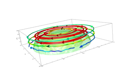
Figure 1: A still frame (at $t\omega_{pe}=235.2$, when the magnetic fields saturate) from a movie (multimedia view), showing the evolution of three contours of density, and a selection of magnetic field lines generated by the Biermann mechanism (from $t\omega_{pe}=0$ to $298.2$). This data is taken from the 3D simulation presented in Paper I Schoeffler et al. (2014) in which $L_{T}/d_{e}=50$ with $m_{i}/m_{e}=25$.

In Fig. 1 a still frame from a movie (multimedia view) is shown, which illustrates this generation of magnetic fields via the Biermann battery, with perpendicular temperature and density gradients in a 3D PIC simulation. The profiles generating these gradients are explained in section V. Three contours of density of the expanding plasma are displayed along with Biermann generated magnetic field lines at a time after the magnetic fields have grown and saturated. (This is from the 3D simulation presented in Paper I Schoeffler et al. (2014); here, $L/d_{e}=50$ and $m_{i}/m_{e}=25$.) The movie shows the plasma expanding (at the sound speed) outward as magnetic fields are generated via the Biermann battery mechanism.

III Weibel instability

As we showed in Paper I Schoeffler et al. (2014), the configuration that gives rise to the Biermann Battery also triggers the Weibel instability Weibel (1959) for $L/d_{e}>100$. Note, only the temperature gradient is essential for this effect. This instability is caused by pressure anisotropies, and thus is an intrinsically kinetic effect. The anisotropy in this paper is due to the kinetic evolution of a temperature gradient in a collisionless system, the details of which will explained in a forthcoming publication. Unlike the Biermann battery, the Weibel instability must start from a seed magnetic field. This seed field may be generated by the Biermann battery, or from small scale fluctuations found in both PIC simulations and in nature, due to finite numbers of particles (referred to as shot noise in electronics Schottky (1918)).

To get a quantitative understanding of what is expected from such an instability, let us consider an initial plasma with a bi-Maxwellian velocity distribution:

$$f_{0\alpha}=n_{\alpha}v_{th\perp\alpha}^{-2}v_{th\parallel\alpha}^{-1}\left(2\pi\right)^{-3/2}\exp\left(-\frac{v_{\perp\alpha}^{2}}{2v_{th\perp\alpha}^{2}}-\frac{v_{\parallel\alpha}^{2}}{2v_{th\parallel\alpha}^{2}}\right),$$ (6)

where the thermal velocity is larger in one direction deemed as parallel $v_{th\parallel\alpha}>v_{th\perp\alpha}$, with $v_{th(\perp,\parallel)\alpha}\equiv\sqrt{T_{(\perp,\parallel)\alpha}/m_{\alpha}}$. The $\alpha$ index represents each of the particle species.

The dispersion relation of an unmagnetized collisionless plasma with this distribution can be obtained from the Vlasov equation. The solution for electromagnetic perturbations consists of the following expression Weibel (1959):

$$k_{\perp}^{2}c^{2}-\omega^{2}-\sum_{\alpha}\omega_{p\alpha}^{2}A_{\alpha}-\sum_{\alpha}\omega_{p\alpha}^{2}\left(A_{\alpha}+1\right)\xi_{\alpha}Z\left(\xi_{\alpha}\right)=0$$ (7)

where $k_{\perp}$ is the wavenumber, $\omega_{p\alpha}$ is the plasma frequency, $A_{\alpha}\equiv T_{\parallel\alpha}/T_{\perp\alpha}-1$ is the temperature anisotropy, $\xi_{\alpha}=\omega/\sqrt{2}k_{\perp}v_{th\perp\alpha}$, and $Z\left(\right)$ is the plasma dispersion function Fried and Conte (1961). For the purposes of this paper we assume that the ions do not play a role because of their large masses and low temperature and thus we will drop the $\alpha$ index; however, in systems with larger ion temperatures, they may play an important role on longer timescales, especially if the electron anisotropy is not present due to collisions. In this study, the instability is based on electron physics: the anisotropy is in the electron pressure, and the instability forms at the electron inertial scale $d_{e}$.

There exists a purely imaginary solution where $\omega=i\gamma$ as long as the normalized perturbation wavenumber $kd_{e}<\sqrt{A}$. This unstable growing mode is referred to as the Weibel instability, and is driven by the anisotropy $A$. Although we have described this instability in the context of a bi-Maxwellian distribution, similar physics is present for a wide range of velocity distributions with a larger velocity spread in the parallel direction. For example, delta functions Fried (1959), waterbag distributions Yoon and Davidson (1987), and kappa distributions Zaheer and Murtaza (2007) all yield similar solutions. We will later use the bi-Maxwellian solution to quantitatively check the growth rates and wavelengths found in our simulation.

IV Computational Model

Using the OSIRIS framework Fonseca et al. (2002, 2008), we perform a set of particle-in-cell (PIC) simulations to investigate the generation and amplification of magnetic fields via the Biermann battery. We use the same initialization for our simulations as in Paper I Schoeffler et al. (2014), a simplification of the aforementioned laser-plasma systems. The fluid velocity, electric field, and magnetic field are initially uniformly zero.

We start with a spheroid distribution of density, that has a shorter length scale in one direction:

$$\begin{array}[]{l}n=\begin{cases}(n_{0}-n_{b})\cos(\pi R_{1}/2L_{T})+n_{b},&\mbox{if }R_{1}<L_{T},\\ n_{b},&\mbox{otherwise},\end{cases}\\ \\ \mbox{where }R_{1}=\sqrt{x^{2}+(L_{T}/L_{n}y)^{2}+z^{2}},\end{array}$$ (8)

$n_{0}$ is the reference density, and $n_{b}=0.1n_{0}$ is a uniform background density. As in section II, the characteristic lengths of the temperature and density gradients are denoted by $L_{T}$ and $L_{n}$, respectively. To represent the newly formed plasma bubble, which is flatter in the direction of the laser, $z$, we set $L_{T}/L_{n}=2$ (this is a generic choice that appears to be qualitatively consistent with experiments, e.g. Nilson et al. (2006); Li et al. (2007); Kugland et al. (2012); note, however, that the specific value of $L_{T}/L_{n}$ depends on target and laser properties and thus can vary). Although this is the initial density, and can in principle change with time, it does not evolve much during our simulations: the density expands at the sound speed $c_{s}$ and all simulations are run with $t\ll L_{n}/c_{s}$.

The initial velocity distributions are Maxwellian, with a uniform ion thermal velocity, $v_{th0i}$. The spatial profile for the electron thermal velocity is cylindrically symmetric along the $z$ direction where it is hottest in the center. This is implemented in a similar manner to the density:

$$\begin{array}[]{l}v_{the}=\begin{cases}(v_{th0e}-v_{thbe})\cos(\pi R_{2}/2L_{T})+v_{thbe},&\mbox{if }R_{2}<L_{T},\\ v_{thbe},&\mbox{otherwise},\end{cases}\\ \\ \mbox{where }R_{2}=\sqrt{x^{2}+z^{2}},\end{array}$$ (9)

resulting in a maximum initial electron pressure, $P_{e0}=m_{e}n_{0}v_{th0e}^{2}$. (Paper I Schoeffler et al. (2014) mistakenly stated $P_{e0}=m_{e}n_{0}v_{th0e}^{2}/2$.) The numerical values of these thermal velocities are: $v_{th0e}=0.2c$ and $v_{th0i}=v_{thbe}=0.01c$. It is important to note that unlike the density profile, the temperature profile changes significantly with time: the peak drops by a factor of $\sim 2$, and the temperature gradient driving the Biermann battery vanishes after an electron transit time. This means we should expect agreement with Eq. (4) and not Eq. (5).

We will normalize the magnetic field for the results of this paper as $B/\sqrt{8\pi P_{e0}}=\beta_{e}^{-1/2}$, time as $t\omega_{pe}$ where $\omega_{pe}\equiv\sqrt{4\pi n_{0}e^{2}/m_{e}}$, and distance as $x/d_{e}$ where $d_{e}\equiv c/\omega_{pe}$. Unlike the previous definition of $\omega_{pe}$, this uses the peak density $n_{0}$, so for regions where $n<n_{0}$, the local inverse electron beta, inverse plasma frequency, and electron inertial length are larger than the normalization indicates.

For simplicity the boundaries are periodic, but the box is large enough that they do not interfere with the dynamics. The dimensions of the simulation domain range from $-L,L$ in both $x$ and $y$ (and $z$ in 3D), where $L=15/8L_{T}$. The spatial resolution is $8$ grid points/$d_{e}$ or $1.6$ grid points/$\lambda_{d}$, where $\lambda_{d}$ is the Debye length (This resolution is the same as that used in Paper I Schoeffler et al. (2014), which mistakenly reported 16 grid points/$d_{e}$). The time resolution is $\Delta t\omega_{pe}=0.07$. The 2D simulations have 64 particles per grid cell (ppg), and the 3D simulation has 27 ppg.

V Insensitivity to mass ratio

In order to investigate a larger range of $L_{T}/d_{i}$, the simulations presented in Paper I Schoeffler et al. (2014) were run with a reduced mass ratio of $25$. In order to test the dependence of the values reported there on mass ratio, we simulate with a mass ratio of $100$, $400$, and the more realistic $2000$. (In most astrophysical contexts, the mass ratio would be the 1836 of Hydrogen, while laser experiments have a larger value.)

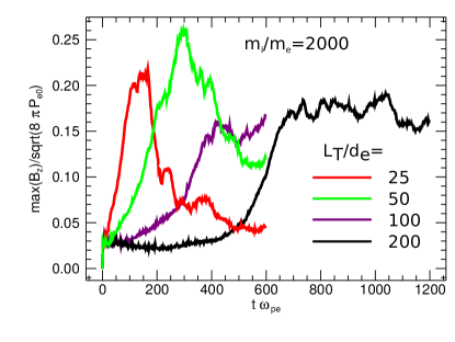
Figure 2: Maximum magnetic field $B_{z}$ vs. time for a selection of system sizes ($L_{T}/d_{e}$) with $m_{i}/m_{e}=2000$. This figure shows the same qualitative behavior as figure 3(a) in Paper I Schoeffler et al. (2014). The results of the simulation with $L_{T}/d_{e}=400$ are presented in Fig. 8.

In Fig. 2, the maximum magnetic field is displayed versus time for various system sizes, $L_{T}/d_{e}$. This plot is equivalent to Figure 3(a) in Paper I Schoeffler et al. (2014), now using a realistic mass ratio of $m_{i}/m_{e}=2000$. There is no qualitative difference between the realistic mass and the simulations done in Paper I Schoeffler et al. (2014) with $m_{i}/m_{e}=25$. For the simulations with $L_{T}/d_{e}=25$ and $50$, the magnetic field strength reaches a peak and decays away due to the ion acoustic instability Haines (1997). This instability is stronger at larger mass ratio, and thus still relevant at the larger $L_{T}/d_{e}=50$. For $L_{T}/d_{e}=100$ and $200$, the magnetic field saturates around its peak value. These are equivalent to the results found for $m_{i}/m_{e}=25$. The growth of the field occurs about $8$ times faster than predicted in Eq. (2). This is an effect of our particular choice of a density profile. The derivation of Eq. (2) assumes $\bm{\nabla}n/n=1/L_{n}$, while more precisely $\bm{\nabla}n/n=n_{0}/n(\bm{x})L_{n}$, and for our profile $n_{0}/n(\bm{x})=8$ at the location of fastest magnetic field growth.

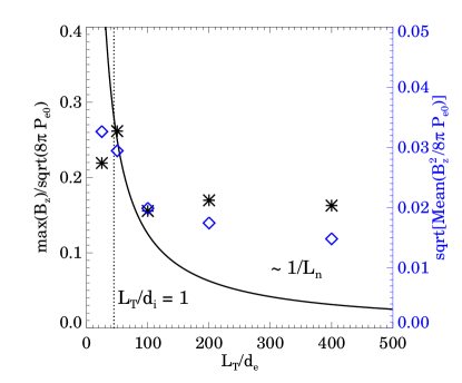
Figure 3: Maximum (black asterisks), and average magnitude (blue diamonds) of the magnetic field, $B_{z}$, vs. $L_{T}/d_{e}$ with $m_{i}/m_{e}=2000$ at the time, $t\omega_{pe}$, when the magnetic field reaches a maximum. The solid black curve indicates a scaling of $\sim 1/L_{n}$ (exactly $6.25d_{e}/L_{n}$), and the dotted line indicates where $L_{T}/d_{i}=1$.

In Fig. 3 we present the scaling of maximum and average magnitude (the square root of $B_{z}^{2}$ averaged in a box $2L_{T}\times 2L_{n}$ surrounding the expanding bubble) of the saturated magnetic field (or peak magnetic field for $L_{T}/d_{e}\leq 50$) as a function of system size. This is equivalent to Figure 3(b) in Paper I Schoeffler et al. (2014), but with $m_{i}/m_{e}=2000$. Much like the $m_{i}/m_{e}=25$ case, Fig. 3 shows three regions; one where the Biermann magnetic field growth is suppressed by microinstabilities (the peak field is suppressed for $L/d_{e}=25$), a regime that scales as $d_{e}/L_{T}$ ($\approx 8d_{e}/\sqrt{2}L_{T}\approx 6.25d_{e}/L_{T}$) after a peak around $L_{T}/d_{i}=1$, and a Weibel dominated regime for $L/d_{e}\geq 100$. In contrast to the purely Biermann prediction where the saturated magnetic field vanishes at large $L_{T}$, in the Weibel dominated regime the saturated magnetic field strength remains finite for large system sizes, confirming the conclusions obtained for $m_{i}/m_{e}=25$ in Paper I Schoeffler et al. (2014). The numerical trends shown in Fig. 3 suggest that the magnetic field amplitude at saturation in the Weibel regime is independent of $L_{T}$. This is compatible with existing understanding on the saturation of the Weibel instability Davidson et al. (1972); Califano et al. (1998); Silva et al. (2003). The presented magnitude of the saturated magnetic field is slightly larger than shown in Paper I Schoeffler et al. (2014) ($\beta_{e}\approx 32$ instead of $100$) (see also Fig. 5). Note that at the location of maximum $B$, the local thermal velocity is close to $1/2v_{th0e}$ and the local density close to $1/4n_{0}$. Therefore, the value of $\beta_{e}$ at that location is $\beta_{e}\approx 2$.

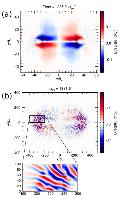
Figure 4: Out-of-plane magnetic field $B_{z}$ at peak magnitude with $m_{i}/m_{e}=2000$ for, (a) $L_{T}/d_{e}=50$ (Biermann regime) at $t\omega_{\text{pe}}=235.2$, and (b) $L_{T}/d_{e}=400$ (Weibel regime) at $t\omega_{\text{pe}}=1881.6$, and zoom-in of Weibel fields showing $kd_{e}\approx 0.2$ (wavelength $\lambda/d_{e}\approx 31.4$).

The distinction between the Weibel and Biermann regimes is evident where the saturated magnetic field strength stops following the $d_{e}/L_{T}$ scaling, but it can be more clearly seen when observing the structure of the magnetic fields in space for each simulation. A plot of the out-of-plane magnetic field is shown in Fig. 4, for $L_{T}/d_{e}=50$, and $400$. In the Biermann regime, shown in Fig. 4(a) ($L_{T}/d_{e}=50$), the spatial structures of the magnetic field are at the system size, and follow the structures of the initial density and temperature profiles. The Weibel regime, on the other hand, seen in Fig. 4(b) ($L_{T}/d_{e}=400$), exhibits small ($kd_{e}\approx 0.2$) magnetic structures consistent with the Weibel instability. These observations are qualitatively the same as shown in Figure 2 of Paper I Schoeffler et al. (2014). The length scale of the initial Weibel filaments is also consistent with the magnetic spectra, which is presented (for $m_{i}/m_{e}=25$) in Figure 5 of Paper I Schoeffler et al. (2014) showing a peak at $kd_{e}\approx 0.2$.

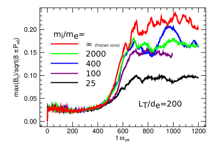
Figure 5: Maximum magnetic field $B_{z}$ vs. time for a selection of mass ratios ($m_{i}/m_{e}$) at $L_{T}/d_{e}=200$ (Weibel regime).

Assuming the mass ratio is sufficiently large, the Weibel instability is independent of mass ratio, because it is based on electron dynamics that act at timescales much faster than the ions. We thus expect the saturated magnetic field to asymptote as the mass ratio increases. To verify this we performed a scan in mass ratio for the $L_{T}/d_{e}=200$ case, which is in the Weibel regime, but computationally small enough to perform several simulations. In Fig. 5 we show that the magnitude of the magnetic field is only weakly dependent on the mass ratio. Although it changes in magnitude by a factor of $2$ from $m_{i}/m_{e}=25$ to $100$, with larger mass ratios the saturated magnetic field appears to asymptote. There is little difference even for frozen ions where the effective mass ratio is infinite. In addition, we find that the length scales of the magnetic perturbations are insensitive to mass ratio.

VI Evidence for the Weibel instability

In Paper I Schoeffler et al. (2014) we have shown evidence of the development of the Weibel instability in simulations of expanding plasmas with perpendicular temperature and density gradients. Here we further show that the simulation results exhibit excellent agreement with theoretical predictions of both the growth rate and wavenumber for the Weibel instability.

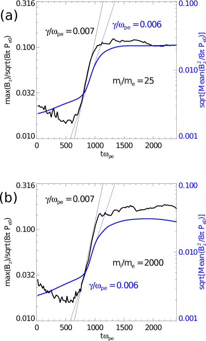
Figure 6: Maximum (black curve) and average magnitude (blue curve) of magnetic field $B_{z}$ vs. time for $L_{T}/d_{e}=400$, with $m_{i}/m_{e}=$ (a) $25$, and (b) $2000$. This plot shows the respective growth rates (of the instability identified as the Weibel instability) corresponding to $\gamma/\omega_{pe}=0.007$ and $0.006$.

Looking at the time evolution of the growth of the magnetic fields, we are able to measure the growth rate of the instability producing the small scale magnetic fields ($kd_{e}\approx 0.2$) observed in our simulations. In Fig. 6, for the $L_{T}/d_{e}=400$ simulation where we claim the magnetic fields are dominated by the Weibel instability, the measured growth rate of the maximum and average magnetic field is $\gamma/\omega_{pe}=0.007$, and $0.006$ respectively. We find the same measured growth rate for both the smaller mass ratio $m_{i}/m_{e}=25$ shown in Fig. 6(a), and the more realistic $m_{i}/m_{e}=2000$ in Fig. 6(b), consistent with our expectation that the plasma dynamics we are observing are due to the electrons, not the ions.

We can test these observed growth rates and wavenumbers by comparing their values to that predicted by theory, namely, the fastest growing mode calculated from Eq. (7). This is only a rough estimate of the instability because there are density and temperature gradients in the simulation, and the velocity distributions have evolved, and are likely not bi-Maxwellian. However, these factors should not significantly influence the result. As stated in section III, similar solutions exist for a variety of distribution functions, and at the scale of the Weibel instability, the variation of temperature and density due to the background gradients is negligible. The parameters of Eq. (7) are: $A$, $v_{th\perp e}$, and the local plasma frequency $\omega_{pe}$, which depends on the local plasma density $n$. One of the outputs of OSIRIS is the thermal spread (of the electrons) in the $x$ and $y$ directions, $v_{thex}$ and $v_{they}$. This allows us to measure $A=v_{th\parallel e}^{2}/v_{th\perp e}^{2}-1$ along $y=0$ where $v_{thex}=v_{th\parallel e}$, and $v_{they}=v_{th\perp e}$. In addition, we measure $n$ so that we can solve the dispersion relation numerically from Eq. (7) at each position along $x$. We calculate the predicted $\gamma$ for a range of $k$, so that we can obtain the fastest growing $\gamma$ and the associated $k$.

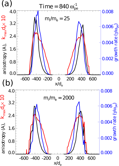
Figure 7: Anisotropy ($A$) (black curve), $k_{max}d_{e}$ (red curve), and growth rate ($\gamma/\omega_{pe}$) of the Weibel instability as predicted from Eq. (7) (blue curve), along a cut at $y=0$ at $t\omega_{pe}=840$ for $L_{T}/d_{e}=400$, with $m_{i}/m_{e}=$ (a) $25$, and (b) $2000$.

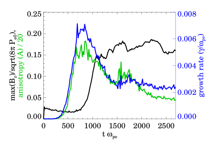
Figure 8: Maximum magnetic field $B_{z}$ (black curve), anisotropy ($A$)/20 (green curve), and growth rate ($\gamma/\omega_{pe}$) of the Weibel instability as predicted from Eq. (7) (blue curve), versus time for $L_{T}/d_{e}=400$, with $m_{i}/m_{e}=2000$.

In Fig. 7 we show a plot of the measured anisotropy $A$, and the calculated $\gamma$ and $k$ of the fastest growing mode, along $y=0$ at $t\omega_{pe}=840$. This is during the time with the largest growth rate $\gamma$ ($t\omega_{pe}\approx 700-1100$, see Fig. 8). Again we find almost equivalent results for the smaller mass ratio $m_{i}/m_{e}=25$ shown in  Fig. 7(a), and the more realistic $m_{i}/m_{e}=2000$ in Fig. 7(b). The maximum growth rate along $x$ is $\gamma/\omega_{pe}\approx 0.007$, which is consistent with the values measured above in Fig. 6. In addition, the calculated $kd_{e}\approx 0.2$ matches the observations, and the locations with the largest growth rate ($|x/d_{e}|\approx 200-400$) are coincident with the Weibel fields visible in Fig. 4(b), and Figure 2(b) of Paper I Schoeffler et al. (2014).

In Fig. 8, like in Fig. 2, we show the maximum magnetic field versus time, now for $L_{T}/d_{e}=400$. In addition we show the maximum measured anisotropy $A$ across $x$ (green curve), and the maximum calculated growth rate $\gamma$ (blue curve). The growth rate $\gamma$ increases with $A$, and peaks at the same time as the magnetic field begins to grow, strongly suggesting the Weibel instability.

To summarize, there is strong evidence that the Weibel instability is generated in our simulations; the growth rate, wavenumber, and the location and time where the fastest growth of the measured instability occur, are consistent with the theoretical predictions.

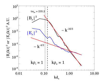
Figure 9: The energy spectrum of the magnetic field $B_{z}$ (black curve), and electric field $E_{x}$ (blue curve), for the 3D simulation ($L_{T}/d_{e}=50$ and $m_{i}/m_{e}=25$) at $t\omega_{pe}=235.2$ (when the magnetic field growth saturates). The dotted line indicates where $k\rho_{i}=1$, and the dashed line where $k\rho_{e}=1$, below which power law behaviors are predicted, with a slope of $-16/3$ for magnetic energy, and $-4/3$ for electric energy, as shown in the solid red curves Schekochihin et al. (2009). [Note that in this simulation $\rho_{i}\sim\rho_{e}$ because the temperature ratio $T_{e}/T_{i}=16$ is comparable to the mass ratio.]

VII Gyrokinetic power law spectra

A surprising finding in Paper I Schoeffler et al. (2014) was the agreement of the power law slope of the magnetic energy spectrum at scales below the electron Larmor radius, with gyrokinetic predictions Schekochihin et al. (2009). The prediction is based on energy transferred via a turbulent cascade of kinetic Alfvén waves, which is converted at $k\rho_{e}\sim 1$ via electron Landau damping into an entropy cascade.

For the 3D run that was reported in Paper I Schoeffler et al. (2014), where $L_{T}/d_{e}=50$, the dominant magnetic field is generated by the Biermann battery. This magnetic field (shown in Fig. 1) acts as a guide field on which kinetic Alfvén waves may propagate, damp, and generate the predicted cascade.

In Fig. 9, we show the magnetic and electric energy spectra for this run. The spectra are obtained by performing a Fourier transform over the entire system for one component of the electric or magnetic fields, and then averaging over all directions of $\bm{k}$. In addition to the $-16/3$ power-law slope of the magnetic energy already revealed in Paper I Schoeffler et al. (2014), we observe that the electric energy spectrum is in good agreement with a $-4/3$ power-law, as predicted Schekochihin et al. (2009). At the time shown, the spectra has reached a steady state and remains unchanged for the rest of the simulation, up to $t\omega_{pe}=298.2$.

VIII Conclusions

We have performed kinetic simulations of plasmas with perpendicular temperature and density gradients of ranging mass ratio up to $m_{i}/m_{e}=2000$, and confirmed the magnetic field generation and amplification shown in Paper I Schoeffler et al. (2014). We have shown that as the system size increases beyond $L_{T}/d_{e}\sim 100$, the major source of magnetic field changes from the Biermann battery mechanism to kinetic Weibel generated fields, which remain finite ($\beta_{e}\sim 1$) for large system sizes. We have done further analysis on the simulations done in Paper I Schoeffler et al. (2014), and on the new simulations with $m_{i}/m_{e}=2000$ confirming that in large system sizes, magnetic fields are generated by the Weibel instability. Finally we have shown that our results agree with gyrokinetic models in power laws found in both electric and magnetic energy spectra.

We reiterate the main applications of our conclusions shown in Paper I Schoeffler et al. (2014), which are significant to the topic of the generation of magnetic fields in astrophysical contexts including shocks found in supernova remnants. Although small scale, the Weibel instability generates magnetic fields at significant levels ($\beta_{e}\sim 1$ independent of $L_{T}$). These are astrophysically relevant magnitudes in typical contexts (where $L_{T}/d_{i}\gg 1$), unlike the fields predicted by the Biermann battery that yield $\beta_{e}\sim(d_{i}/L_{T})^{-2}$. However the discrepancy between the large scales of astrophysical magnetic fields and the microscopic Weibel fields remains. Whether it is possible for a mechanism such as turbulence to bridge this gap remains an outstanding mystery of astrophysical research.

The matching of power law spectra points to the exciting possibility of validating theories of kinetic turbulence in laser experiments. Due to the small scale separation between $L_{T}$, $\rho_{i}$, and $\rho_{e}$ in our 3D simulation, we are only able to measure a sub-$\rho_{e}$ power law. However, the spectra at other scales could potentially be tested in simulations and experiments. In addition to the configuration that we have studied, Weibel-generated turbulence may occur due to anisotropies induced by other mechanisms; for example, laser-generated hot electron beams with return currents. It might be possible to probe such magnetized laser plasmas in order to investigate turbulence at kinetic scales. Indeed, one such an experiment has recently been performed at the Tata Institute of Fundamental Research, Mumbai Mondal et al. (2012), probing the magnetic energy spectra in the range with $\rho_{i}^{-1}\lesssim k<\rho_{e}^{-1}$. A power law of $-7/3$ has been measured from the experimental results (to be published shortly), consistent with theoretical predictions Schekochihin et al. (2009).

In existing (and future) laser-plasma experiments the predicted $1/L$ scalings in Eq. (4) and Eq. (5) of the saturated Biermann magnetic fields should be relevant. Furthermore, it may be possible to find the electron-Weibel instability as we have done here, as long as collisions do not occur faster than the electron transit time and keep the temperature isotropic ($\nu_{ei}L_{T}/v_{the}\ll 1$). Based on experimentally relevant parameters, this condition is equivalent to the following engineering formula:

$$1\times 10^{-2}\left(\frac{n}{1\times 10^{19}\text{ cm}^{-3}}\right)\left(\frac{\ln\Lambda}{10}\right)\left(\frac{L_{T}}{400\mu\text{m}}\right)\left(\frac{T_{e}}{1\text{keV}}\right)^{-2}\ll 1\text{,}$$ (10)

where $n$ is the number density, $\ln\Lambda$ is the Coulomb logarithm, $L_{T}$ is the gradient scale, and $T_{e}$ is the electron temperature. This inequality suggests the possibility of observing the Weibel instability, since the physical values quoted above are reasonable numbers which can occur at the low density, high temperature coronae generated around laser targets, e.g. Gao et al. (2013). Note that in this work the strong temperature gradient is assumed to form before the anisotropy and the subsequent instability. We think this is a good modeling assumption in cases where intense short-pulse lasers are used. Cases with longer, less intense lasers require more careful consideration due to the possible influence of collisions and the laser fields during the timescale of the experiment.

IX Acknowledgments

This work was supported by the European Research Council (ERC-2010-AdG Grant No. 267841). NFL was partially supported by the Fundação para a Ciência e Tecnologia via Grants UID/FIS/50010/2013 and IF/00530/2013. Simulations were carried out at SuperMUC (Germany) under a PRACE grant, and the authors acknowledge the Gauss Centre for Supercomputing (GCS) for providing computing time through the John von Neumann Institute for Computing (NIC) on the GCS share of the supercomputer JUQUEEN at Jülich Supercomputing Centre (JSC).

References

- Kulsrud and Zweibel (2008) R. M. Kulsrud and E. G. Zweibel, Rep. Prog. Phys. 71, 046901 (2008).
- Kulsrud and Anderson (1992) R. M. Kulsrud and S. W. Anderson, Astrophys. J. 396, 606 (1992).
- Brandenburg et al. (2012) A. Brandenburg, D. Sokoloff, and K. Subramanian, Space Sci. Rev. 169, 123 (2012).
- Biermann (1950) L. Biermann, Z. Naturforsch. 5a, 65 (1950).
- Weibel (1959) E. S. Weibel, Phys. Rev. 114, 18 (1959).
- Stamper et al. (1971) J. A. Stamper, K. Papadopoulos, R. N. Sudan, S. O. Dean, and E. A. McLean, Phys. Rev. Lett. 26, 1012 (1971).
- Li et al. (2006) C. K. Li, F. H. Séguin, J. A. Frenje, J. R. Rygg, R. D. Petrasso, R. P. J. Town, P. A. Amendt, S. P. Hatchett, O. L. Landen, A. J. MacKinnon, et al., Phys. Rev. Lett. 97, 135003 (2006).
- Gao et al. (2015) L. Gao, P. M. Nilson, I. V. Igumenshchev, M. G. Haines, D. H. Froula, R. Betti, and D. D. Meyerhofer, Phys. Rev. Lett. 114, 215003 (2015).
- Schoeffler et al. (2014) K. M. Schoeffler, N. F. Loureiro, R. A. Fonseca, and L. O. Silva, Phys. Rev. Lett. 112, 175001 (2014).
- Max et al. (1978) C. E. Max, J. J. Thomson, and W. M. Manheimer, Phys. Fluids 21, 128 (1978).
- Craxton and Haines (1978) R. S. Craxton and M. G. Haines, Plasma Phys. 20, 487 (1978).
- Haines (1997) M. G. Haines, Phys. Rev. Lett. 78, 254 (1997).
- Schottky (1918) W. Schottky, Ann. Phys. 362, 541 (1918).
- Fried and Conte (1961) B. D. Fried and S. D. Conte, The Plasma Dispersion Function (Academic Press, New York, 1961).
- Fried (1959) B. D. Fried, Phys. Fluids 2, 337 (1959).
- Yoon and Davidson (1987) P. H. Yoon and R. C. Davidson, Phys. Rev. A 35, 2718 (1987).
- Zaheer and Murtaza (2007) S. Zaheer and G. Murtaza, Phys. Plasmas 14, 022108 (2007).
- Fonseca et al. (2002) R. A. Fonseca, L. O. Silva, F. S. Tsung, V. K. Decyk, W. Lu, C. Ren, W. B. Mori, S. Deng, S. Lee, T. Katsouleas, and J. C. Adam, Lect. Notes Comput. Sci. 2331, 342 (2002).
- Fonseca et al. (2008) R. A. Fonseca, S. F. Martins, L. O. Silva, J. W. Tonge, F. S. Tsung, and W. B. Mori, Plasma Phys. Contr. Fusion 50, 124034 (2008).
- Nilson et al. (2006) P. M. Nilson, L. Willingale, M. C. Kaluza, C. Kamperidis, S. Minardi, M. S. Wei, P. Fernandes, M. Notley, S. Bandyopadhyay, M. Sherlock, R. J. Kingham, M. Tatarakis, Z. Najmudin, W. Rozmus, et al., Phys. Rev. Lett. 97, 255001 (2006).
- Li et al. (2007) C. K. Li, F. H. Seguin, J. A. Frenje, J. R. Rygg, R. D. Petrasso, R. P. J. Town, O. L. Landen, J. P. Knauer, and V. A. Smalyuk, Phys. Rev. Lett. 99, 055001 (2007).
- Kugland et al. (2012) N. L. Kugland, D. D. Ryutov, P.-Y. Chang, R. P. Drake, G. Fiksel, D. H. Froula, S. H. Glenzer, G. Gregori, M. Grosskopf, M. Koenig, Y. Kuramitsu, C. Kuranz, M. C. Levy, E. Liang, et al., Nat. Phys. 8, 809 (2012).
- Davidson et al. (1972) R. C. Davidson, D. A. Hammer, I. Haber, and C. E. Wagner, Phys. Fluids 15, 317 (1972).
- Califano et al. (1998) F. Califano, F. Pegoraro, S. V. Bulanov, and A. Mangeney, Phys. Rev. E 57, 7048 (1998).
- Silva et al. (2003) L. O. Silva, R. A. Fonseca, J. W. Tonge, J. M. Dawson, W. B. Mori, and M. V. Medvedev, Astrophys. J. Lett. 596, L121 (2003).
- Schekochihin et al. (2009) A. A. Schekochihin, S. C. Cowley, W. Dorland, G. W. Hammett, G. G. Howes, E. Quataert, and T. Tatsuno, Astrophys. J. Suppl. Ser. 182, 310 (2009).
- Mondal et al. (2012) S. Mondal, V. Narayanan, W. J. Ding, A. D. Lad, B. Hao, S. Ahmad, W. M. Wang, Z. M. Sheng, S. Sengupta, P. Kaw, A. Das, and G. R. Kumar, Proc. Nat Acad. Scai. U.S.A. 109, 8011 (2012).
- Gao et al. (2013) L. Gao, P. M. Nilson, I. V. Igumenschev, G. Fiksel, R. Yan, J. R. Davies, D. Martinez, V. Smalyuk, M. G. Haines, E. G. Blackman, D. H. Froula, R. Betti, and D. D. Meyerhofer, Phys. Rev. Lett. 110, 185003 (2013).