Hybrid cluster-expansion and density-functional-theory approach for optical absorption in TiO₂

Abstract

A combined approach of first-principles density-functional calculations and the systematic cluster-expansion scheme is presented. The dipole, quadrupole, and Coulomb matrix elements obtained from ab initio calculations are used as an input to the microscopic many-body theory of the excitonic optical response. To demonstrate the hybrid approach for a nontrivial semiconductor system, the near-bandgap excitonic optical absorption of rutile TiO₂ is computed. Comparison with experiments yields strong evidence that the observed near-bandgap features are due to a dipole-forbidden but quadrupole-allowed $1s$-exciton state.

I Introduction

The single-particle electronic states are the basis needed to quantitatively model the excitonic optical properties of a semiconductor system Yu and Cardona (2010); Haug and Koch (2009); Kira and Koch (2012); Mahan (2000). In many cases, we can use semiempirical methods like the $\mathbf{k}\cdot\mathbf{p}$ theory together with the effective-mass approximation Kane (1966); Yu and Cardona (2010); Haug and Koch (2009); Kira and Koch (2012) to obtain the electronic wave functions and energies. However, there are many systems which are not characterized well enough for the needed input parameters to be reliably known. These kinds of ”nontrivial” systems are found, for example, in novel semiconductor materials containing more than two constituents, like ternary, quaternary and even more complex compounds Vurgaftman et al. (2001), in dilute bismides or nitrides Broderick et al. (2012); Vurgaftman and Meyer (2003), in organic systems, in organic/inorganic heterostructures, and in complex interfaces Coakley and McGehee (2004); Graetzel et al. (2012).

Even seemingly simple binary systems such as bulk rutile TiO₂ pose considerable challenges. At first sight, TiO₂ seems to be a common semiconductor material that has been widely used in applications and intensively studied over several decades Fujishima et al. (2008); DeVore (1951); Grant (1959); Pascual et al. (1977); Amtout and Leonelli (1995); Chiodo et al. (2010); Migani et al. (2014). Despite this, after a second look, one quickly realizes that TiO₂ clearly belongs into the class of nontrivial systems mentioned above, because many of its essential parameters are poorly known. For example, the reported conduction-band effective mass in rutile varies almost two orders of magnitude Pascual et al. (1977); Madelung et al. (2000); Zhang et al. (2014). Additionally, it exhibits an exceptionally large refractive index in the visible range as well as particularly strong birefringence and dispersion properties DeVore (1951); Grant (1959).

Furthermore, rutile has highly asymmetric dielectric properties regarding different crystallographic directions with a particularly large magnitude of the low-frequency dielectric constant Madelung et al. (2000). This results in an exceptionally strong screening of the Coulomb interaction between electrons and holes for excitons with a binding energy below or comparable to the polar phonon energies Bechstedt (2015). Nevertheless, optical absorption measurements Pascual et al. (1977, 1978); Amtout and Leonelli (1992a, b, 1995) near the band gap of TiO₂ have shown some indications of excitonic features which, however, are very controversially discussed in the literature. For example, the excitonic signatures were interpreted as a dipole-forbidden but quadrupole-allowed $1s$ exciton Pascual et al. (1977, 1978), or as a weakly dipole-allowed $2p$ exciton state Amtout and Leonelli (1992a, b, 1995).

In order to study the optical properties of rutile and to develop a general scheme that allows us to overcome the restrictions of the semiempirical models, we have to use more systematic methods to access the microscopic properties of the electronic states. Here, the most widely used scheme is density functional theory (DFT) Hohenberg and Kohn (1964); Kohn and Sham (1965), which has been proven to be a very efficient approach in obtaining ground-state properties for various solid-state systems, molecules, nanostructures, liquids, and molecules adsorbed on surfaces Martin (2004); Engel and Dreizler (2011).

The DFT computed single-particle energies and wave functions can then be used as an input to the cluster-expansion scheme Kira and Koch (2006a, 2012) that provides first-principles level description of many-body dynamics. Its strength relies on a systematic grouping of different correlations as clusters that build up sequentially in time Kira and Koch (2012). The cluster-expansion method is widely applied in semiconductor solid-state systems Richter et al. (2009); Witzany et al. (2011); Harsij et al. (2012); Leymann et al. (2013); Almand-Hunter et al. (2014); Leymann et al. (2015); Suwa et al. (2014) and it even can describe quantum-optical properties Kira and Koch (2006b); *PhysRevA.78.022102 as well as strongly interacting Bose gas Kira (2014); *kira2015hyperbolic; *kira2015coherent quantitatively.

In this work, we combine a DFT approach with the cluster-expansion method to obtain a hybrid cluster-expansion and density-functional-theory (CE-DFT) scheme for studying dynamical many-body quantum phenomena. We first obtain the needed Coulomb and optical matrix elements via DFT for the second-quantization system Hamiltonian that we then use to model dynamical effects by applying the cluster-expansion scheme. The electronic excitation dynamics are derived in a very general form, yielding a structure similar to the semiconductor Bloch equations Lindberg and Koch (1988); Haug and Koch (2009). Prior to our work, ab initio matrix elements have been used together with the semiconductor Bloch equations to compute the surface exciton properties on a Si surface Reichelt et al. (2003). Linear optical properties such as the absorption follow directly once the dynamics have been solved. We then apply our combined CE-DFT method for rutile TiO₂ and study its near-bandgap optical properties by considering electric-dipole, electric-quadrupole, and magnetic-dipole light–matter interactions. We also show that the electric-quadrupole interaction is highly dependent on the propagation and polarization directions of the light. We use our microscopic results to analyze the experimentally available absorption spectra Pascual et al. (1977, 1978); Amtout and Leonelli (1992a, b, 1995), finding a good level of agreement that allows us to identify the observed excitonic signature as a dipole-forbidden but quadrupole-allowed $1s$ exciton.

II Theoretical Background

To effectively formulate the quantum kinetics of a semiconductor system via the cluster-expansion method, we start from a generic Hamiltonian Kira and Koch (2012, 2006a)

$$H= \sum_{i}E_{i}\,a^{\dagger}_{i}{a}_{i}-E(t)\sum_{i,j}\,F_{ij}\,a^{\dagger}_{i}{a}_{j}$$

$$+\frac{1}{2}\sum_{i,i^{\prime},j,j^{\prime}}V_{ii^{\prime};j^{\prime}j}\,a^{\dagger}_{i}a^{\dagger}_{i^{\prime}}{a}_{j^{\prime}}{a}_{j},$$ (1)

where $a^{\dagger}_{i}$ (${a}_{i}$) is the creation (annihilation) operator of an electronic state defined by the particle index $i$ and $E(t)$ is the time-dependent electric field. This Hamiltonian is uniquely defined by $E_{i}$, $F_{ij}$, and $V_{ii^{\prime};j^{\prime}j}$, i.e., by the energies of the electronic states and the matrix elements for light–matter and electron–electron interactions, respectively.

To identify these input parameters from a DFT calculation, we repeat the derivation of Eq. (II) from the Lagrangian and Hamiltonian formalism of classical electrodynamics Cohen-Tannoudji et al. (1997). In the Coulomb gauge, the quantization yields the conventional minimal-substitution Hamiltonian for electronic quasiparticles Kira and Koch (2012); Kira et al. (1999):

$$H_{N}= \sum_{i=1}^{N}\bigg{\{}\frac{1}{2m_{0}}\left[\mathbf{p}_{i}-e\mathbf{A}(\mathbf{r}_{i},t)\right]^{2}+U(\mathbf{r}_{i})\bigg{\}}$$

$$\quad+\frac{1}{2}\sum_{i\neq j}V(\mathbf{r}_{i},\mathbf{r}_{j}),$$ (2)

where $m_{0}$ is the free-electron mass, $e$ is the charge of an electron, $\mathbf{A}(\mathbf{r},t)$ is the vector potential of an optical field, $U(\mathbf{r})$ is an external potential, and $V(\mathbf{r},\mathbf{r}^{\prime})$ is a pairwise electron–electron interaction.

Equation (II) includes a contribution proportional to the square of the optical field that can be eliminated via the Power-Zienau-Woolley transformation Cohen-Tannoudji et al. (1997); Keller (2011) in our initial Coulomb-gauge Lagrangian. This way, we obtain a classical Hamiltonian where the light–matter interaction is directly given by the electric $\mathbf{E}(\mathbf{r},t)$ and the magnetic $\mathbf{B}(\mathbf{r},t)$ fields instead of the vector potential. After quantization, it reads

$$H^{\prime}_{N}= \sum_{i=1}^{N}H(\mathbf{p}_{i},\mathbf{r}_{i})-E(t)\sum_{j=1}^{N}F(\mathbf{p}_{i},\mathbf{r}_{i})$$

$$+\frac{1}{2}\sum_{i\neq j}V(\mathbf{r}_{i},\mathbf{r}_{j})+H_{\text{RM}},$$ (3)

where we assumed fields of the form $\mathbf{E}(t,\mathbf{r})=E(t)\mathbf{E}(\mathbf{r})$ and $\mathbf{B}(t,\mathbf{r})=E(t)\mathbf{B}(\mathbf{r})/\omega$ with the optical frequency $\omega$. The diamagnetic contributions Cohen-Tannoudji et al. (1997); Keller (2011) $H_{\text{RM}}$ can be neglected at moderate field intensities, hence we omit this term in the following. The single-particle Hamiltonian is given by

$$H(\mathbf{p},\mathbf{r})=\frac{\mathbf{p}^{2}}{2m_{0}}+U(\mathbf{r}),$$ (4)

and the light–matter-interaction operator by

$$F(\mathbf{p},\mathbf{r})=-e\mathbf{r}\cdot\sum_{n=0}^{\infty}\frac{1}{(n+1)!}[(\mathbf{r}\cdot\nabla_{\mathbf{r}^{\prime}})^{n}\,\mathbf{E}(\mathbf{r}^{\prime})]_{\mathbf{r}^{\prime}=0}$$

$$-\frac{e}{2m_{0}}\sum_{l=0}^{\infty}\frac{l+1}{(l+2)!}\Big{\{}\mathbf{p}\cdot\Big{[}\mathbf{r}\times[(\mathbf{r}\cdot\nabla_{\mathbf{r}^{\prime}})^{l}\,\mathbf{B}(\mathbf{r}^{\prime})]\Big{]}$$

$$+\Big{[}\mathbf{r}\times[(\mathbf{r}\cdot\nabla_{\mathbf{r}^{\prime}})^{l}\,\mathbf{B}(\mathbf{r}^{\prime})]\Big{]}\cdot\mathbf{p}\Big{\}}_{\mathbf{r}^{\prime}=0},$$ (5)

after expressing $\mathbf{E}(\mathbf{r})$ and $\mathbf{B}(\mathbf{r})$ through their multipole expansions. The electric-dipole interaction ($n=0$) can be weak, especially near the direct band gap of TiO₂ Pascual et al. (1977, 1978). To keep our approach general while simultaneously suitable for near-bandgap optical properties of TiO₂, we initially consider all terms within the multipole expansions of $\mathbf{E}(\mathbf{r})$ and $\mathbf{B}(\mathbf{r})$.

If we know the electronic wave functions $\phi_{i}(\mathbf{r})$ and energies $E_{i}$ that follow from the Schrödinger equation

$$H(\mathbf{p},\mathbf{r})\,\phi_{i}(\mathbf{r})=E_{i}\,\phi_{i}(\mathbf{r}),$$ (6)

we can construct the fermionic field operator

$$\hat{\Psi}(\mathbf{r})=\sum_{i}\phi_{i}(\mathbf{r})\,{a}_{i}.$$ (7)

As elaborated in many text books Mahan (2000); Kira and Koch (2012); Haug and Koch (2009), we can use $\hat{\Psi}(\mathbf{r})$ in the second-quantization step for $H(\mathbf{p},\mathbf{r})$, $F(\mathbf{p},\mathbf{r})$, and $V(\mathbf{r},\mathbf{r}^{\prime})$ to obtain the Hamiltonian (II) from Eq. (II) with the matrix elements

$$F_{ij}= \int d^{3}r\,\phi^{*}_{i}(\mathbf{r})\,F(\mathbf{p},\mathbf{r})\,\phi^{*}_{j}(\mathbf{r}),$$ (8)

$$V_{ii^{\prime};j^{\prime}j}= \int d^{3}rd^{3}r^{\prime}\,\phi^{*}_{i}(\mathbf{r})\phi^{*}_{i^{\prime}}(\mathbf{r}^{\prime})V(\mathbf{r},\mathbf{r}^{\prime})\phi_{j^{\prime}}(\mathbf{r}^{\prime})\phi_{j}(\mathbf{r}).$$ (9)

In principle, $\phi_{i}(\mathbf{r})$ could be chosen to be any complete orthonormal set for the second-quantization step. In practice, it is useful if they are eigenfunctions of a suitable effective Hamiltonian that is known to give eigenvalues $E_{i}$ corresponding to accurate ionization energies and electron affinities. A possible choice is a DFT Hamiltonian with a scissor shift to obtain the correct band gap, even better would be to use a scissor shifted static $GW$ Hamiltonian if it is available (we avoid explicit frequency dependence in the single-particle Hamiltonian in order to keep the time evolution simple and ensure orthogonal wave functions). The unshifted Hamiltonian can be written by replacing the potential $U(\mathbf{r})$ with

$$U[\rho_{0}](\mathbf{r})=V_{\text{ext}}(\mathbf{r})+V_{\text{H}}[\rho_{0}](\mathbf{r})+V_{\text{xc}}[\rho_{0}](\mathbf{r}),$$ (10)

where the external potential from the nuclei $V_{\text{ext}}(\mathbf{r})$ is augmented with an effective potential that includes the interaction of the electrons with the average electron density $V_{\text{H}}[\rho_{0}](\mathbf{r})$, as well as approximate exchange and correlation effects $V_{\text{xc}}[\rho_{0}](\mathbf{r})$. Note that these terms are explicitly dependent on the equilibrium density matrix $\rho_{0}$ that is determined in DFT by a self-consistent iterative procedure. To correct the band gap we shift the eigenvalues by a downshift for the states below the Fermi level and an upshift on the states above it. The terms we have added to $U(\mathbf{r})$ include some Coulomb terms that must be later subtracted when we develop the equations of motion as we discuss in Appendix A.

One of the most critical conditions for the success of our CE-DFT method is that the computed $\phi_{i}(\mathbf{r})$ and $E_{i}$ are sufficiently close to the actual one-particle wave function and energies, respectively. When we assume that this condition is fulfilled, by utilizing Eqs. (8) and (9), we obtain a DFT-defined system Hamiltonian (II) that is the basis of our hybrid CE-DFT approach.

III CE-DFT equation for optical absorption

It is beneficial to divide the electronic index $i$ in Eq. (II) into two parts $i\rightarrow(\lambda,j)$ where $\lambda=v$ or $\lambda=c$ for states that are either occupied or unoccupied in the ground state of the system, respectively, and $j$ defines the exact state inside these groups. After we have constructed our DFT-defined system Hamiltonian $H$, we can study the dynamics of the expectation values $P^{\lambda\lambda^{\prime}}_{ij}\equiv\langle a^{\dagger}_{\lambda,i}{a}_{\lambda^{\prime},j}\rangle$ via the Heisenberg equation of motion and the cluster-expansion method Kira and Koch (2006a, 2012). This yields the semiconductor Bloch equations

$$i\hbar\frac{\partial}{\partial t}P^{\lambda\lambda^{\prime}}_{ij}= \sum_{k}\big{[}\tilde{E}^{\lambda^{\prime}}_{kj}\,P^{\lambda\lambda^{\prime}}_{ik}-\tilde{E}^{\lambda}_{ik}\,P^{\lambda\lambda^{\prime}}_{kj}+\Omega^{\lambda}_{ik}\,P^{\bar{\lambda}\lambda^{\prime}}_{kj}$$

$$-\Omega^{\bar{\lambda}^{\prime}}_{kj}\,P^{\lambda\bar{\lambda}^{\prime}}_{ik}\big{]}+\Gamma^{\lambda\lambda^{\prime}}_{ij},$$ (11)

where $\tilde{E}^{\lambda}_{ij}$ ($\Omega^{\lambda}_{ij}$) is the renormalized kinetic energy (Rabi frequency) and $\bar{\lambda}$ denotes the complement of $\lambda$ ($\bar{v}=c$ and $\bar{c}=v$). Explicit forms of $\tilde{E}^{\lambda}_{ij}$ and $\Omega^{\lambda}_{ij}$ can be found in Appendix A. The term $\Gamma^{\lambda\lambda^{\prime}}_{ij}$ includes the coupling to the higher-order clusters that follows from the two-particle contributions Kira and Koch (2006a, 2012) due to Coulomb and phonon interactions.

Similarly to the formulation of Eq. (III), we can construct equations for higher order clusters and study, e.g., dynamics of exciton correlations Kira and Koch (2006a, 2012). However, in this work we focus on fundamental aspects of combining DFT and the cluster-expansion method, thus limiting our considerations on the level of Eq. (III).

In this situation, Eq. (III) yields a closed set of equations between the dynamics of the microscopic polarization $P_{ij}\equiv P^{vc}_{ij}$, the electron occupation $f^{e}_{ij}\equiv P^{cc}_{ij}$, and the hole occupation $f^{h}_{ij}\equiv\delta_{ij}-P^{vv}_{ij}$. Even though this set of equations can be used to model many interesting dynamical effects such as nonlinearities or excitation induced changes in the optical response, in the present study we concentrate on the linear absorption properties of the rutile TiO₂ system.

In this case, $f^{e}_{ij}=f^{h}_{ij}=0$ in Eq. (III) and we can neglect several terms that are connected to optical nonlinearities. When we also make the Tamm-Dancoff approximation Onida et al. (2002) by omitting processes that would generate coupling between the $P^{vc}_{ij}$ and $P^{cv}_{ij}$ terms, Eq. (III) reduces to (see Appendix A for details)

$$i\hbar\frac{\partial}{\partial t}P_{ij}= [E^{c}_{j}-E^{v}_{i}]P_{ij}-\sum_{k,l}{\mathcal{V}}^{vc;cv}_{kj;li}\,P_{kl}$$

$$-E(t)\,F^{cv}_{ji}+\Gamma^{vc}_{ij},$$ (12)

containing

$${\mathcal{V}}^{\lambda_{1}\lambda_{2};\lambda_{3}\lambda_{4}}_{i_{1}i_{2};i_{3}i_{4}}\equiv V^{\lambda_{1}\lambda_{2};\lambda_{3}\lambda_{4}}_{i_{1}i_{2};i_{3}i_{4}}-V^{\lambda_{2}\lambda_{1};\lambda_{3}\lambda_{4}}_{i_{2}i_{1};i_{3}i_{4}},$$ (13)

where we have grouped the direct and exchange electron–electron interactions under a single matrix element. Here, we use a notation where the $\lambda$ index in the matrix elements is written as a superscript above the corresponding $i$ index, e.g., $E^{v}_{i}\equiv E_{v,i}$. While Eq. (III) can be used for any system defined by the Hamiltonian (II) and when rotating-wave contributions dominate the dynamics, Eq. (III) is applicable only in cases where the Tamm-Dancoff approximation is justified.

The homogeneous solution of Eq. (III) defines the Wannier equation Kira and Koch (2012); Haug and Koch (2009)

$$[E^{c}_{j}-E^{v}_{i}]\phi_{\nu}(i,j) -\sum_{k,l}{\mathcal{V}}^{vc;cv}_{kj;li}\,\phi_{\nu}(k,l)$$

$$=E_{\nu}\,\phi_{\nu}(i,j),$$ (14)

as an eigenvalue problem for the wave function $\phi_{\nu}(i,j)$ and the energy $E_{\nu}$ of an exciton state $\nu$. Converting the polarization into the exciton basis,

$$P_{ij}=\sum_{\nu}p_{\nu}\,\phi_{\nu}(i,j),\quad p_{\nu}=\sum_{i,j}\phi^{*}_{\nu}(i,j)\,P_{ij},$$ (15)

the Fourier transform of Eq. (III) yields

$$[\hbar\omega+i\gamma_{\nu}(\omega)]p_{\nu}(\omega)=E_{\nu}\,p_{\nu}(\omega)-{\mathcal{F}}_{\nu}\,E(\omega),$$ (16)

where $E(\omega)$ is the Fourier transform of $E(t)$ and

$${\mathcal{F}}_{\nu}\equiv\sum_{i,j}\phi^{*}_{\nu}(i,j)\,F^{cv}_{ji}$$ (17)

defines a generalized oscillator strength of optical transitions.

To avoid a detailed analysis of Coulomb and phonon scattering, we introduce a dephasing function

$$\gamma_{\lambda}(\nu)=\frac{\gamma_{\nu}}{\exp[(E_{\nu}-\hbar\omega-\mu_{\nu})/\Delta E_{\nu}]+1}$$ (18)

that phenomenologically includes the contributions of the $\Gamma^{vc}_{ij}$ term in Eq. (16). With the parameters $\gamma_{\nu}$, $\mu_{\nu}$, and $\Delta E_{\nu}$, function $\gamma_{\nu}(\omega)$ describes the excitation-induced dephasing effects Kira and Koch (2006a); Smith et al. (2010) as well as the exponential decay of the absorption tail towards lower energies; a phenomenon known as the Urbach tail Haug and Koch (2009); Kurik (1971), which is of particularly significance in polar semiconductors Liebler and Haug (1991) like TiO₂.

We can now solve Eq. (16) directly, yielding

$$p_{\nu}(\omega)=\frac{{\mathcal{F}}_{\nu}}{E_{\nu}-\hbar\omega-i\gamma_{\nu}(\omega)}E(\omega).$$ (19)

The absorption response of our system then follows from the imaginary part of the linear susceptibility Kira and Koch (2012) $\chi(\omega)=\frac{P(\omega)}{\epsilon_{0}E(\omega)}$ where $P(\omega)=\sum_{\nu}{\mathcal{F}}_{\nu}^{*}\,p_{\nu}(\omega)$ is the macroscopic polarization. With the help of Eq. (19), the Elliott formula for the optical absorption becomes

$$\alpha(\omega) \equiv\frac{\omega}{nc}\text{Im}[\chi(\omega)]$$

$$=\frac{\omega}{\epsilon_{0}nc}\sum_{\nu}\frac{|{\mathcal{F}}_{\nu}|^{2}\,\gamma_{\nu}(\omega)}{(E_{\nu}-\hbar\omega)^{2}+\gamma^{2}_{\nu}(\omega)},$$ (20)

where $n$ is the refractive index of the material.

IV Excitonic absorption in rutile

IV.1 Two-band model

To apply the general results of the previous section for TiO₂, we assume a three-dimensional crystal having an infinite volume. Then, the potential $U(\mathbf{r})$ in the Hamiltonian (4) must have the periodicity of the lattice, and we can use the Bloch theorem to produce electronic wave functions of the form

$$\phi_{\lambda,\mathbf{k}}(\mathbf{r})=\frac{e^{i\mathbf{k}\cdot\mathbf{r}}}{(2\pi)^{3/2}}\,u_{\lambda,\mathbf{k}}(\mathbf{r}),$$ (21)

where $u_{\lambda,\mathbf{k}}(\mathbf{r})$ is a lattice-periodic Bloch function, $\mathbf{k}$ is the wave vector, and $\lambda$ denotes different Bloch bands. Thus, in the main step before constructing the system Hamiltonian (II) of our crystal, we solve the band structure $E^{\lambda}_{\mathbf{k}}$ and the Bloch functions $u_{\lambda,\mathbf{k}}(\mathbf{r})$ corresponding to the Schrödinger equation (6) via DFT, requiring the form of Eq. (21).

Our DFT results presented in Sec. IV.4 reveal that it is well justified to model the near-bandgap optical properties of TiO₂ by including only the energetically lowest conduction band $\lambda=c$ and the highest valence band $\lambda=v$. Hence, we can relate the Bloch-band index $\lambda$ and the $\lambda$ index of Sec. III and directly use Eqs. (III)-(17) if we replace the sums over the particle index by $k$-space integrals. Furthermore, in the vicinity of the band gap $E_{g}$ we find (see Sec. IV.4) that the electron energy $E^{e}_{\mathbf{k}}\equiv E^{c}_{\mathbf{k}}-E_{g}$ and the hole energy $E^{h}_{\mathbf{k}}\equiv-E^{v}_{\mathbf{k}}$ are accurately described by a parabolic dispersion

$$E^{\lambda}_{\mathbf{k}}=\frac{\hbar^{2}}{2m^{\lambda}_{x}}k_{x}^{2}+\frac{\hbar^{2}}{2m^{\lambda}_{y}}k_{y}^{2}+\frac{\hbar^{2}}{2m^{\lambda}_{z}}k_{z}^{2},$$ (22)

where $m^{\lambda}_{i}$ is the $i$-directional effective mass of an electron or hole for $\lambda=e$ or $\lambda=h$, respectively.

IV.2 Light–matter interaction

When we express $\mathbf{E}(\mathbf{r})$ and $\mathbf{B}(\mathbf{r})$ in Eq. (II) via their multipole expansions, the matrix element in Eq. (8) is related to the position operator $\mathbf{r}$. In our crystal system, the position operator $\mathbf{r}$ maps a wave function by $\mathbf{r}\phi_{\lambda,\mathbf{k}}(\mathbf{r})$ out of the Hilbert space that is constructed by the lattice-periodic wave functions Resta (1999). Consequently, the $\mathbf{r}$ matrix element is not uniquely defined and, for example, in DFT computations its value depends on how we chose the unit cell of a system Gu et al. (2013). This is a known problem that has been widely studied in connection with the electric-dipole matrix element over several decades Yafet (1957); Blount (1962); Resta (1994); Gu et al. (2013) and is still an important research topic Swiecicki and Sipe (2014).

In general, while the light–matter matrix element in Eq. (8) is not directly observable, it manifests itself through other quantities like the oscillator strength ${\mathcal{F}}_{\nu}$. By considering $F^{\lambda\lambda^{\prime}}_{\mathbf{k}\mathbf{k}^{\prime}}$ in Eq. (17) for an infinite crystal under the assumption that a two-band model with a parabolic band structure is valid, we present in Appendix B a method where the ambiguities related to the $\mathbf{r}$ matrix elements can be avoided by expressing the light–matter matrix elements via the momentum matrix element $\mathbf{p}^{\lambda\lambda^{\prime}}_{\mathbf{k}}$. Using our DFT Bloch functions, these matrix elements are computed via

$$\mathbf{p}^{\lambda\lambda^{\prime}}_{\mathbf{k}}\equiv\frac{1}{\Omega_{0}}\int_{\Omega_{0}}d^{3}r\,u^{*}_{\lambda,\mathbf{k}}(\mathbf{r})\,\mathbf{p}\,u_{\lambda^{\prime},\mathbf{k}}(\mathbf{r}),$$ (23)

with the unit cell volume $\Omega_{0}$.

Even though we discuss in Appendix B how our approach can be used to solve $F^{cv}_{\mathbf{k}\mathbf{k}^{\prime}}$ for arbitrary $\mathbf{E}(\mathbf{r},t)$ and $\mathbf{B}(\mathbf{r},t)$, we focus on the electric-dipole, electric-quadrupole, and magnetic-dipole light–matter interactions. Furthermore, we assume that a plane wave with $\mathbf{E}(\mathbf{r})=e^{i\mathbf{q}_{E}\cdot\mathbf{r}}\hat{\mathbf{e}}_{E}$ and $\mathbf{B}(\mathbf{r})=e^{i\mathbf{q}_{E}\cdot\mathbf{r}}(\mathbf{q}_{E}\times\hat{\mathbf{e}}_{E})$ propagates through our sample, where $\mathbf{q}_{E}$ and $\hat{\mathbf{e}}_{E}$ define the wave-vector and the polarization direction of the optical field, respectively. Then, the $n=0$, $n=1$, and $l=0$ terms of Eq. (II) yield the light–matter interaction operators

$$D\equiv -e\hat{\mathbf{e}}_{E}\cdot\mathbf{r},$$ (24)

$$Q\equiv -i\frac{e}{2}(\hat{\mathbf{e}}_{E}\cdot\mathbf{r})(\mathbf{q}_{E}\cdot\mathbf{r}),$$ (25)

$$M\equiv -\frac{e}{2\omega m_{0}}[\mathbf{r}\times(\mathbf{q}_{E}\times\hat{\mathbf{e}}_{E})]\cdot\mathbf{p},$$ (26)

for the electric-dipole, electric-quadrupole and magnetic-dipole interactions, respectively.

By using the steps outlined in Appendix B, we connect the operators $D$, $Q$, and $M$ to the matrix elements

$$D^{cv}_{\mathbf{k}\mathbf{k}^{\prime}}= \delta(\mathbf{k}-\mathbf{k}^{\prime})D^{cv}_{\mathbf{k}},$$ (27)

$$Q^{cv}_{\mathbf{k}\mathbf{k}^{\prime}}= \delta(\mathbf{k}-\mathbf{k}^{\prime})\sum_{i,j}e_{i}\,Q^{cv}_{\mathbf{k};ij}q_{j},$$ (28)

$$M^{cv}_{\mathbf{k}\mathbf{k}^{\prime}}= \delta(\mathbf{k}-\mathbf{k}^{\prime})\sum_{i,j}e_{i}\,M^{cv}_{\mathbf{k};ij}q_{j}.$$ (29)

Here, $e_{i}$ and $q_{i}$ are the $i$-directional components of the vectors $\hat{\mathbf{e}}_{E}$ and $\mathbf{q}_{E}$, respectively, ${D}^{cv}_{\mathbf{k}}=-ie\hat{\mathbf{e}}_{E}\cdot\tilde{\mathbf{p}}^{cv}_{\mathbf{k}}$ includes the conventional Haug and Koch (2009); Kira and Koch (2012); Gu et al. (2013) relation between the $\mathbf{r}$ and $\mathbf{p}$ matrix elements via

$$\tilde{\mathbf{p}}^{\lambda\lambda^{\prime}}_{\mathbf{k}}\equiv\frac{\hbar}{m_{0}}\frac{\mathbf{p}^{\lambda\lambda^{\prime}}_{\mathbf{k}}}{E^{\lambda}_{\mathbf{k}}-E^{\lambda^{\prime}}_{\mathbf{k}}},$$ (30)

and the explicit forms of ${Q}^{cv}_{\mathbf{k};ij}$ and ${M}^{cv}_{\mathbf{k};ij}$ are given in Appendix B. The matrix element $F^{cv}_{\mathbf{k}\mathbf{k}^{\prime}}$ becomes

$$F^{cv}_{\mathbf{k}\mathbf{k}^{\prime}}=\delta(\mathbf{k}-\mathbf{k}^{\prime})(D^{cv}_{\mathbf{k}}+Q^{cv}_{\mathbf{k}}+M^{cv}_{\mathbf{k}}).$$ (31)

IV.3 Coulomb interaction and direct excitonic states

For rutile TiO₂, it is necessary to model the electron–electron interaction $V(\mathbf{r},\mathbf{r}^{\prime})$ using the result for anisotropic media Landau et al. (1984). The resulting expression can be given through the Fourier transformation

$$V(\mathbf{r},\mathbf{r}^{\prime})= \int d^{3}k\,V_{\mathbf{k}}e^{i\mathbf{k}\cdot(\mathbf{r}-\mathbf{r}^{\prime})},$$ (32)

$$V_{\mathbf{k}}= \frac{e^{2}}{8\pi^{3}\varepsilon_{0}}\frac{1}{\epsilon_{x}k_{x}^{2}+\epsilon_{y}k_{z}^{2}+\epsilon_{z}k_{z}^{2}},$$ (33)

where $\varepsilon_{0}$ is the vacuum permittivity, $\epsilon_{i}$ is the dielectric constant along the $i$-directional principal axis of the permittivity tensor Landau et al. (1984) and $k_{i}$ is the related component of the $\mathbf{k}$ vector, respectively. If our system has an excitation in a sufficiently small region of the Brillouin zone, we can quite generally approximate the Coulomb matrix element by

$$V^{\lambda_{1}\lambda_{2};\lambda_{3}\lambda_{4}}_{\mathbf{k}_{1}\mathbf{k}_{2};\mathbf{k}_{3}\mathbf{k}_{4}}=\delta(\mathbf{k}_{1}+\mathbf{k}_{2}-\mathbf{k}_{3}-\mathbf{k}_{4})\delta_{\lambda_{1}\lambda_{4}}\delta_{\lambda_{2}\lambda_{3}}V_{\mathbf{k}_{1}-\mathbf{k}_{4}},$$ (34)

which follows from Eqs. (9), (32), and (33) (see Appendix C and Ref. Bechstedt (2015)). By using $u_{c,\mathbf{k}}(\mathbf{r})$ and $u_{v,\mathbf{k}}(\mathbf{r})$ in TiO₂ determined by DFT computations, we carefully check in Appendix C that the relevant Coulomb interaction is indeed well approximated by the matrix element (34).

Since the light–matter and Coulomb interactions conserve the crystal momentum $\hbar\mathbf{k}$ via the matrix elements in Eqs. (31) and (34), we find from Eq. (III) that only direct quantities $P^{\lambda\lambda^{\prime}}_{\mathbf{k}}\equiv P^{\lambda\lambda^{\prime}}_{\mathbf{k}\mathbf{k}}$ couple to optical excitation if we omit possible nondiagonalities in $\Gamma^{\lambda\lambda^{\prime}}_{\mathbf{k}\mathbf{k}^{\prime}}$. Consequently, we need to consider only the direct excitonic states with wave functions $\phi_{\nu}(\mathbf{k})\equiv\phi_{\nu}(\mathbf{k},\mathbf{k})$ for the optical response following form Eq. (15). These states are solutions of the Wannier equation

$$(E^{c}_{\mathbf{k}}-E^{v}_{\mathbf{k}})\phi_{\nu}(\mathbf{k})-\int d^{3}k^{\prime}\,V_{\mathbf{k}-\mathbf{k}^{\prime}}\,\phi_{\nu}(\mathbf{k}^{\prime})=E_{\nu}\,\phi_{\nu}(\mathbf{k}),$$ (35)

where $\mathbf{k}$ can be associated with the relative motion of electrons and holes, and we have assumed that the approximations in Eqs. (22) and (34) are valid Kira and Koch (2012); Bechstedt (2015). In Eq. (35), the $\nu$ index typically refers to the symmetry of the exciton states with values $\nu=1s$, $2p$, etc. In an anisotropic system, we can assume that this symmetry based grouping is only approximate and the character of, e.g., $s$ and $p$ like states becomes mixed.

Equation (35) can have simultaneously anisotropic energies $E^{\lambda}_{\mathbf{k}}$ and matrix elements $V_{\mathbf{k}}$, which may complicate solution strategies. However, we can always perform a $k$-space coordinate transform in Eq. (35) that results in a transformed spherical Coulomb matrix element (see Appendix D). The use of $V^{\lambda_{1}\lambda_{2};\lambda_{3}\lambda_{4}}_{\mathbf{k}_{1}\mathbf{k}_{2};\mathbf{k}_{3}\mathbf{k}_{4}}$ in Eq. (34) together with this coordinate transformation comprises a rather general and remarkably beneficial approach for modeling properties of anisotropic systems. This is due to the fact that DFT can be effectively used to compute $E^{\lambda}_{\mathbf{k}}$ and $F^{\lambda\lambda^{\prime}}_{\mathbf{k}\mathbf{k}^{\prime}}$ whereas computing all the Coulomb-interaction terms would be a numerically highly demanding task; especially in three-dimensional problems. Furthermore, a spherical Coulomb matrix element makes it possible to solve the excitonic states and the related properties of a system efficiently by using techniques developed elsewhere PS_ . In particular, we expand the excitonic wave functions $\phi_{\nu}(\mathbf{k})$ and all matrix elements in terms of spherical harmonics in the transformed coordinate system and then solve the corresponding high-dimensional eigenvalue problem given by Eq. (35) as discussed in Appendix D and in Ref. PS_ .

IV.4 Band structure

In our numerical evaluations, we first set-up our computational cell based on the experimentally determined Madelung et al. (2000) tetragonal crystal structure of rutile TiO₂ that is defined by the unit cell with lattice constants $a=b=4.59$ Å and $c=2.96$ Å. The inset of Fig. 1(a) depicts the unit cell in a Cartesian coordinate system where oxygen (titanium) atoms are illustrated by the red (gray) spheres.

Starting from this unit cell, we perform a DFT calculation with the SIESTA Soler et al. (2002) code using the PBE exchange-correlation functional Perdew et al. (1996), Trouiller-Martins pseudopotentials Troullier and Martins (1991), and a DZP basis set of atomic-like orbitals with an energy shift parameter of 100 meV. After a sufficient convergence of the ground-state properties (with 11x11x17 $k$ points), we rediagonalize the Kohn-Sham Hamiltonian matrix at the $k$ points we are interested in, obtaining the needed $E^{\lambda}_{\mathbf{k}}$ and $u_{\lambda,\mathbf{k}}(\mathbf{r})$.

To compute the matrix elements in Eqs. (8) and (9), we put the cell-periodic part of the wave functions on a real space grid and Fourier transform them to obtain their plane-wave representation. All needed matrix elements can then be computed either in real or reciprocal space. We use the DFT computed energies to obtain the effective masses, while the light–matter-interaction matrix elements in Eq. (8) are used directly.

Our computed Coulomb matrix elements in Eq. (9) were found to correspond well to the matrix element (34) for the small $(\mathbf{k}_{1}-\mathbf{k}_{4})$-values that are important for excitons and we thus chose to use the latter for simplicity. In addition of confirming the approximation (34), the ab initio Coulomb matrix elements were used in a phase matching procedure to obtain the light–matter-interaction matrix elements that correspond to the phase fixing we do when we adopt the matrix element (34). Following this procedure, we obtain all needed matrix elements for Eq. (II), which establishes the technical basis of our CE-DFT approach in TiO₂.

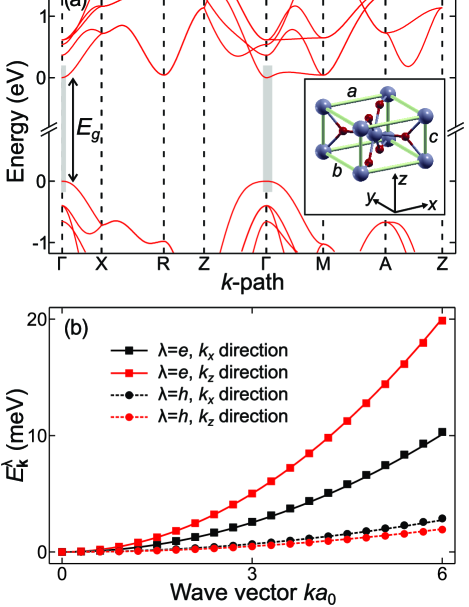
Figure 1: (Color online) Ab initio band structure and its parabolic approximation. (a) A wide region of the ab initio band structure throughout the whole Brillouin zone, where the $k$-space region of interest is indicated by the shaded areas. (b) Electron (solid lines) and hole (dashed lines) energies for $k_{y}=0$ in the region of interest as a function of $k_{x}$ (black lines) and $k_{z}$ (red lines). Parabolic fits for electron and hole energies (lines) approximate ab initio energies (squares and circles) to a high degree of accuracy.

The actual $E^{\lambda}_{\mathbf{k}}$ dispersion obtained from our DFT computations is shown in Fig. 1(a) along the high-symmetry points of the Brillouin zone. The depicted band structure agrees to some extent with multiple previous results Glassford and Chelikowsky (1992); Mo and Ching (1995); Landmann et al. (2012) and indicates a direct gap at the $\Gamma$ point. Our DFT approach with local functionals underestimates the band gap $E_{g}$ by 1.3 eV, which is corrected with the well-known “scissor shift” to produce the experimental $E_{g}=3.03$ eV Pascual et al. (1977); Madelung et al. (2000). However, we use band energies $E^{\lambda}_{\mathbf{k}}$ given directly by our DFT computations in Eq. (30) that is linked to all light–matter-interaction matrix elements.

The shaded rectangles in Fig. 1(a) indicate the electronic states most important for near-bandgap optical transitions, covering roughly a range of 20 meV in electron–hole energy, $E^{c}_{\mathbf{k}}-E^{v}_{\mathbf{k}}$, around the $\Gamma$ point. In this region, the energetically lowest conduction and highest valence band are relatively well separated from the nearby bands such that we can adopt the two-band approach described in Sec. IV.1. Figure 1(b) shows the electron (continuous lines and squares) and the hole energies (dashed lines and circles) near the $\Gamma$ point as a function of $k_{x}$ (black lines) and $k_{z}$ (red lines) when $k_{y}=0$. The reciprocal $k_{x}$, $k_{y}$, and $k_{z}$ directions correspond to lattice $x$, $y$, and $z$ directions, respectively. These directions are selected to be parallel to the $a$, $b$, and $c$ axes of TiO₂ crystal structure, as indicated in the insert of Fig. 1(a).

The computed ab initio $E^{e}_{\mathbf{k}}$ and $E^{h}_{\mathbf{k}}$ energies are almost parabolic in all directions and symmetric with respect to $k_{x}\leftrightarrow k_{y}$ exchange. However, $k_{x}$ (or $k_{y}$) and $k_{z}$ directions exhibit a different $k$ dependence, which creates a strong anisotropy. This anisotropy can be accurately described by Eq. (22) with effective masses $m^{e}_{x}=m^{e}_{y}=1.03m_{0}$, $m^{e}_{z}=0.519m_{0}$, $m^{h}_{x}=m^{h}_{y}=3.80m_{0}$, and $m^{h}_{z}=5.30m_{0}$. Figure 1(b) compares the parabolic model (lines) and the ab initio energies (squares and circles), showing the high accuracy of our approximation. In this figure, the wave vector is scaled by the exciton Bohr radius $a_{0}\equiv 4\pi\epsilon_{0}\epsilon\hbar^{2}/(e^{2}\mu)$ with geometrically averaged reduced mass $\mu\equiv(\mu_{x}^{2}\mu_{z})^{1/3}$ and dielectric constant $\epsilon\equiv(\epsilon_{\perp}^{2}\epsilon_{\parallel})^{1/3}$, where $1/\mu_{i}\equiv 1/m^{e}_{i}+1/m^{h}_{i}$ and we use the low-frequency limit of the dielectric constant tensor of TiO₂ Madelung et al. (2000): $\epsilon_{\perp}=\epsilon_{x}=\epsilon_{y}=111$ and $\epsilon_{\parallel}=\epsilon_{z}=257$.

IV.5 Dipole and quadrupole matrix elements

Figure 2(a) shows the imaginary part of the dipole matrix element $D^{cv}_{\mathbf{k}}$ that we obtain from Eq. (27) with the DFT defined Bloch functions. The real part of $D^{cv}_{\mathbf{k}}$ is negligible. We have selected a $x$-polarized light mode, $\hat{\mathbf{e}}_{E}\parallel\hat{\mathbf{x}}$, and then computed $D^{cv}_{\mathbf{k}}$ along the $k_{x}$ axis (black line), $k_{y}$ axis (red line), and direction $k(\hat{\mathbf{k}}_{x}+\hat{\mathbf{k}}_{y})$ (blue line). In the $k$-space region of interest, the dipole matrix element becomes almost linearly dependent on $k_{x}$. The black line indicates that this dependency is not completely linear due to the visible nonlinearity for $|ka_{0}|>3$. In the $k_{xy}$ direction (blue line), $D^{cv}_{\mathbf{k}}$ remains linear even far away from the $\Gamma$ point.

It follows from the linear-in-$k_{x}$-like dependency that $D^{cv}_{\mathbf{k}}$ remains small along the $k_{y}$ axis (red line) and includes only a minor dependency on $k_{z}$ near the $\Gamma$ point. The dipole matrix element for the $y$-polarized light mode, $\hat{\mathbf{e}}_{E}\parallel\hat{\mathbf{y}}$, is essentially equal to the $\hat{\mathbf{e}}_{E}\parallel\hat{\mathbf{x}}$ matrix element with a sign change and with respect to the $k_{x}\leftrightarrow k_{y}$ transformation. In the immediate vicinity of the $\Gamma$ point, our results indicate that the dipole matrix element for $z$-polarized light modes, $\hat{\mathbf{e}}_{E}\parallel\hat{\mathbf{z}}$, is negligible, yielding a vanishing near-bandgap absorption in TiO₂ for this particular light polarization, as already found in several works Pascual et al. (1978); Amtout and Leonelli (1995).

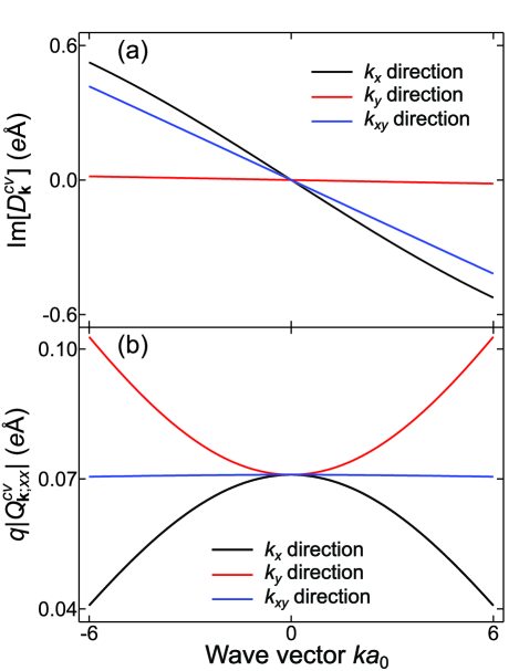
Figure 2: (Color online) Electric-dipole and quadrupole matrix elements. (a) For $x$-polarized light the dipole matrix element $D^{cv}_{\mathbf{k}}$ is almost linear in $k_{x}$ (black line) and even more linear along the $k_{xy}$ direction (blue line) while $D^{cv}_{\mathbf{k}}$ is negligible along the $k_{y}$ axis (red line). (b) The absolute value of the quadrupole matrix element $Q^{cv}_{\mathbf{k};xx}$ is constant along the $k_{xy}$ direction (blue line) and has parabolic dependence along the $k_{x}$ (black line) and $k_{y}$ (red line) axes.

In Fig. 2(b), we show the absolute value of the $Q^{cv}_{\mathbf{k};xx}$ element of the quadrupole-matrix tensor multiplied by the wave number $q=E_{g}n_{o}/(\hbar c)$ where $c$ is the speed of light in vacuum and $n_{o}=2.95$ is the ordinary refractive index of TiO₂ DeVore (1951), corresponding to a light mode polarized in the $xy$ plane. We have used the same color scheme as in Fig. 2(a). In the region of interest, the $q|Q^{cv}_{\mathbf{k},xx}|$ remains constant along the $k_{xy}$ direction while it has a parabolic behavior along the $k_{x}$ and $k_{y}$ axes.

In the vicinity of the $\Gamma$ point, all other components of the quadrupole and magnetic-dipole matrix-element tensors are at least two orders of magnitude smaller than $Q^{cv}_{\mathbf{k};xx}$. The only exception is the $Q^{cv}_{\mathbf{k};yy}$ counterpart of $Q^{cv}_{\mathbf{k};xx}$ (obtained from $Q^{cv}_{\mathbf{k};xx}$ via the $k_{x}\leftrightarrow k_{y}$ transformation). Due to their small magnitude, the other elements play only a minor role for the near-bandgap optical properties of TiO₂. Nevertheless, we still include them in our numerical computations. The large difference in the magnitudes of the different components of the $Q^{ij}_{\mathbf{k}}$ tensor indicates that the near-bandgap quadrupole light–matter interaction in TiO₂ should become highly dependent on the propagation and polarization directions of light. Due to the complicated nature of the electric-dipole, electric-quadrupole, and magnetic-dipole matrix elements, we take them as a direct input from the DFT without any approximations.

IV.6 Optical absorption

Figure 3(a) shows the optical absorption spectrum following from Eq. (III) when we use the low-frequency values $\epsilon_{\perp}=111$ and $\epsilon_{\parallel}=257$ to describe the dielectric screening of Coulomb interaction between electrons and holes in Eq. (33). We have chosen the polarization of light to be always in the $xy$ plane whereas we change the polar $\theta$ and azimuthal $\varphi$ angles that are the angles of propagation with respect to the $z$ and $x$ axes of the unit cell, respectively. Here, we present the absorption spectrum for four sets of $(\theta,\varphi)$ combinations.

Whenever light propagates in the $x$, $y$, or $z$ planes, e.g., in the cases denoted by $(\theta=0,\varphi=0)$ (shaded area) and $(0,\pi/4)$ (black line) in Fig. 3(a), the $Q^{cv}_{\mathbf{k};xx}$ and $Q^{cv}_{\mathbf{k};yy}$ elements of the quadrupole matrix-element tensor do not contribute to the light–matter interaction. Consequently, the absorption spectrum then practically follows only from the electric-dipole interaction. Since the $D^{cv}_{\mathbf{k}}$ matrix elements for $x$- and $y$-polarized light are almost linear in $k_{x}$ and $k_{y}$, respectively, the electric-dipole interaction couples light predominantly to the $p_{xy}$-like excitonic states of the $xy$ plane Pascual et al. (1977, 1978); Amtout and Leonelli (1995). From the $xy$-plane symmetry of our system, it follows that these $p_{xy}$ states are degenerate and by changing the angles $\theta$ and $\varphi$ we cannot drastically change their combined contribution to the optical response, which is shown by the comparison of the spectra labeled $(0,0)$ and $(0,\pi/4)$ in Fig. 3(a). Thus, the major propagation- and polarization-angle dependent changes in our absorption spectrum (for $xy$ polarization) must follow from the quadrupole interaction.

Figure 3: (Color online) Propagation and polarization angle dependency of absorption for polarization in $xy$ plane. (a) When light propagates parallel to the z axis (shaded area and black line), absorption follows from the electric-dipole interaction that does not have strong dependency on the azimuthal angle $\varphi$. Changing the propagation direction into the $xy$ plane (blue and red curves), the strength of the quadrupole interaction can be tuned by varying $\varphi$, yielding notable changes in the spectrum. (b) The resonance strength of the $1s$ exciton as a function of the polar angle $\theta$ when $\varphi=\pi/4$ (black line) and as a function of $\varphi$ with a fixed $\theta=\pi/2$ (red line).

In Fig. 3(a), we also show two spectra denoted as $(\pi/2,\pi/8)$ (blue line) and $(\pi/2,\pi/4)$ (red line) in which the propagation direction points away from the $x$, $y$, or $z$ planes. When comparing the spectra $(0,0)$ and $(\pi/2,\pi/8)$, we see that while the overall absorption intensity is slightly increased, a weak resonance at the spectral position of the $1s$ exciton appears. This transition is dipole-forbidden but quadrupole-allowed Pascual et al. (1977, 1978); Amtout and Leonelli (1995). These trends are further strengthened when the azimuth angle is increased to $\varphi=\pi/4$, yielding the $(\pi/2,\pi/4)$ set with the strongest quadrupole resonance.

In Fig. 3(b), we study how the peak intensity of the $1s$ state changes as a function of the angles $\theta$ and $\varphi$ that give the spectra labeled as $(\theta,\pi/4)$ (black line) and $(\pi/2,\varphi)$ (red line), respectively. More generally, whenever $\theta$ ($\varphi$) is varied we find that $\varphi=\pi/4$ ($\theta=\pi/2$) gives the strongest $1s$ intensity. As a summary, we show the angle dependency of the $1s$-peak intensity in Fig. 3(b), varying only one angle at a time while fixing the other. The shape of these curves follows almost identically the corresponding angular dependency of $|Q^{cv}_{00}|^{2}$.

Even with the most optimal angle combination $(\pi/2,\pi/4)$ for the quadrupole interaction, the resulting excitonic absorption signature is still weaker than the experimentally observed feature Pascual et al. (1977, 1978); Amtout and Leonelli (1992a, b, 1995). This is explained by the extremely small binding energy of $E^{B}_{1s}=0.5$ meV ($E^{B}_{2p_{xy}}=0.1$ meV) for the $1s$ ($2p_{xy}$) exciton due to the unusually large dielectric constants $\epsilon_{\perp}=111$ and $\epsilon_{\parallel}=257$. Additionally, the experimentally measured continuum absorption intensity around 2 meV above the band gap has been reported to be between 25 cm^-1 and 50 cm^-1 Pascual et al. (1977, 1978); Amtout and Leonelli (1995), i.e., our result differ from this roughly by a factor of five.

Generally, it is not obvious whether we should use a low-frequency, a high-frequency or some other phenomenological value of a dielectric constant when we model optical excitations in semiconductors Bechstedt (2015). This is of particularly significance in TiO₂ where the difference between high-frequency constants Madelung et al. (2000) ($\epsilon_{\perp}^{\infty}=6.8$ and $\epsilon_{\parallel}^{\infty}=8.4$) and low-frequency constants ($\epsilon\perp^{0}=111$ and $\epsilon\parallel^{0}=257$) is exceptionally large. In rutile, the contributions of the different sources to the screening of the Coulomb interaction, e.g., phonons and the ionic nature of TiO₂ Persson and Ferreira da Silva (2005), are poorly known Chiodo et al. (2010).

If we adjust the components of the dielectric constant between the high and low frequency values via $\epsilon_{i}(w)=\epsilon^{0}_{i}-(\epsilon^{0}_{i}-\epsilon^{\infty}_{i})w$, where $w$ is between 0 and 1, we can change the binding energies of excitons so that they become visible in the optical spectra. In the inset of Fig 4(b), we show how the binding energies of $1s$ (black line) and $2p$ (red line) change as a function of $\epsilon(w)=[\epsilon_{\perp}^{2}(w)\epsilon_{\parallel}(w)]^{1/3}$. By selecting either $\epsilon(w)=24.3$ or $\epsilon(w)=47.8$, we can tune the absorption to show a distinct resonance 4 meV below the band gap. Effectively, we have adjusted the binding energies of either the $2p_{xy}$ or $1s$ state being the origin of that signature.

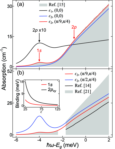
Figure 4: (Color online) Experiments vs. modeled absorption. (a) Computed absorption spectrum with $\epsilon(w)=24.3\equiv\epsilon_{1}$ (black line, scaled down by dividing with $10$) has a drastically different general shape than what is observed in the experiments of Ref. Amtout and Leonelli (1995) (shaded area) and its intensity is one order of magnitude too strong. With $\epsilon(w)=47.8=\epsilon_{2}$ and light propagation parallel to $z$ axis (blue line), the shape and magnitude of the continuum absorption corresponds to the experiment. Changing the propagation to $\theta=\pi/9$ and $\varphi=\pi/4$ (red line), we can achieve similar excitonic feature as in the experiment via $1s$ exciton. (b) Spectrum computed with $\epsilon_{2}$, $\theta=\pi/9$, and $\varphi=\pi/4$ (red line) also agrees well with other experiments in Ref. Pascual et al. (1977) (black line) and in Ref. Pascual et al. (1978) (shaded area). With the angle that supports the most strongest quadrupole interaction (blue line), we find a clear $1s$-exciton resonance. (inset) The $1s$ and $2p_{xy}$ binding energies as a function of $\epsilon$.

In Fig. 4, we compare absorption spectra for different $(\theta,\varphi)$ sets of propagation angles and dielectric constants to the available experiments. If we choose $(0,0)$ and $\epsilon(w)=24.3$ [black line in Fig. 4(a)], the experimental resonance from Ref. Amtout and Leonelli (1995) (shaded area) is assigned to the $2p$ exciton. However, the general shape of the spectrum does not correspond to the measured one, i.e., the $2p$ resonance is too strong compared to the continuum absorption. This trend is strengthened when $\epsilon(w)$ is decreased. In general, whenever the $2p$ resonance is clearly separable from the continuum tail, its ratio to the continuum absorption is too high.

Our analysis shows that the shape of the full bandedge absorption spectrum does not match the experimental observations if we try to model the excitonic signature via the $2p$ state, based on three compelling facts. First, if we assume that the band energies can be described in the form of Eq. (22), $\epsilon(w)$ and the effective masses become connected via Eq. (35). If we change the value of $\epsilon(w)$, we not only describe the screening of electron–electron interaction phenomenologically but also correct possible errors in our effective masses. Second, without considering $\epsilon(w)$, we can assume that our Coulomb matrix element is highly accurate and cannot contribute to this problem, as discussed in Appendix C. Hence, the only remaining uncertainty is in the light–matter matrix elements. Thirdly, since both the $2p$-resonance and the continuum absorption (dominantly) originate from the same source (dipole interaction), possible errors in the dipole matrix element $D^{cv}_{\mathbf{k}}$ would lead only to the scaling of both features with the same factor without a change of the general shape of the spectrum. Thus, based on our results it seems to be practically impossible to model the experimentally observed excitonic feature via $2p$ states.

No such problems occur if we model the excitonic resonance as the $1s$ state by selecting $\epsilon(w)=47.8$, yielding $E^{B}_{1s}=4.0$ meV and $E^{B}_{2p_{xy}}=1.0$ meV. Interestingly, the experimentally obtained Pascual et al. (1977, 1978) binding-energy difference between $1s$ and $2p$ states of 3 meV is well reproduced with these values. Further, selecting the propagation angles $(0,0)$ [blue line in Fig 4(a)], we find that our continuum absorption has the same shape and intensity as in the experiment with a high accuracy. By changing the propagation angle, we can tune the intensity of the $1s$ resonance without drastically changing the shape of the continuum absorption. With a rather small angle of $\theta=\pi/9$ and the optimal $\varphi=\pi/4$ (red line), we find an extremely good agreement to the spectrum of Ref. Amtout and Leonelli (1995).

We also compare our results against other experiments from Refs. Pascual et al. (1977) and Pascual et al. (1978) in Fig. 4(b). Again, we show $(\pi/9,\pi/4)$ with $\epsilon(w)=47.8$ (red line) and additionally $(\pi/2,\pi/4)$ with $\epsilon(w)=47.8$ (blue line). Once more, the excitonic resonance is reproduced with great precision. The continuum absorption of both sets settles in-between the ones from Ref. Pascual et al. (1977) (black line) and Ref. Pascual et al. (1978) (shaded area). As previously, the quadrupole interaction of the $(\pi/2,\pi/4)$ produces the highest intensity for the $1s$ resonance that is now roughly seven times stronger than in the experiments.

In Fig. 4, the band gaps for experimental data have been fixed so that the spectral position of the excitonic resonance matches with the result of Ref. Amtout and Leonelli (1995), where the resonance is located at $\hbar\omega=3.03$ eV. For our theoretical results, we do essentially the same by using the scissor shifted $E_{g}=3.034$ eV. In results of Figs. 3 and 4, we have selected the scattering function $\gamma_{\nu}(\omega)$ in Eq. (18) to be $\gamma_{1s}(\omega)=0.8$ meV for our $1s$ states, producing a similar shape and linewidth broadening for the modeled $1s$ resonance as seen for the experimental resonance. For all the other excitonic states, we use $\gamma_{\nu}=1.8$ meV and $\mu_{\nu}=\Delta E_{\nu}=1.2$ meV. With these selections we mimic the excitation-induced dephasing Kira and Koch (2006a); Smith et al. (2010), without drastically altering location and intensities of our resonances compared to a case $\gamma_{\nu}(\omega)=\gamma_{\nu}$, but reproduce the experimentally detected Tang et al. (1995) steep decay of the continuum absorption tail in rutile TiO₂.

V Summary

In summary, we systematically combine DFT and the cluster-expansion approach to compute the excitonic optical properties of semiconductors. More specifically, the matrix elements needed for microscopic modeling are computed via DFT while the many-body problem is solved with the cluster expansion. We apply this hybrid approach for rutile TiO₂ and compute its near-bandgap optical absorption, following from the electric-dipole, electric-quadrupole and magnetic-dipole light–matter interactions. Our results show that the quadrupole interaction in rutile is highly dependent on the propagation and polarization direction of light. Furthermore, we find that it is hard to explain the experimentally detected excitonic signature in the absorption spectrum of TiO₂ by considering only electric-dipole interaction and the dipole-allowed $2p$ exciton. We obtain an excellent agreement between modeled and experimental spectra through the quadrupole interaction and the quadrupole-allowed $1s$ exciton if the light is propagating in a sufficiently large angle with respect to the crystallographic axes of TiO₂. Hence, the hybrid CE-DFT method seems to be a very promising approach to model many-body effects in semiconductors, opening a wide range of new possibilities to study and utilize properties of nontrivial systems.

VI Acknowledgment

We thank John E. Sipe for helpful discussions. This work is funded by the Deutsche Forschungsgemeinschaft via the SFB 1083. DSP also acknowledges support from Spanish MINECO (Grant MAT2013-46593-C6-2-P).

Appendix A Renormalized terms

The exact form of the renormalized kinetic energy $\tilde{E}^{\lambda}_{ij}$ and the renormalized Rabi frequency $\Omega^{\lambda}_{ij}$ appearing in Eq. (III) are given by

$$\tilde{E}^{\lambda}_{ij}= \delta_{ij}E^{\lambda}_{i}-E(t)D^{\lambda\lambda}_{ji}+\sum_{k,l}\Big{[}{\mathcal{V}}^{\lambda\lambda;\lambda\lambda}_{jk;li}P^{\lambda\lambda}_{kl}+{\mathcal{V}}^{\lambda\bar{\lambda};\bar{\lambda}\lambda}_{jk;li}P^{\bar{\lambda}\bar{\lambda}}_{kl}$$

$$+{\mathcal{V}}^{\lambda\lambda;\bar{\lambda}\lambda}_{jk;li}P^{\lambda\bar{\lambda}}_{kl}+{\mathcal{V}}^{\lambda\bar{\lambda};\lambda\lambda}_{jk;li}P^{\bar{\lambda}\lambda}_{kl}\Big{]}-{\mathcal{V}}^{E;\lambda}_{ji}\,,$$ (36)

$$\Omega^{\lambda}_{ij}= E(t)D^{\bar{\lambda}\lambda}_{ji}-\sum_{k,l}\Big{[}{\mathcal{V}}^{\bar{\lambda}\lambda;\bar{\lambda}\lambda}_{jk;li}P^{\lambda\bar{\lambda}}_{kl}+{\mathcal{V}}^{\bar{\lambda}\lambda;\lambda\lambda}_{jk;li}P^{\lambda\lambda}_{kl}$$

$$+{\mathcal{V}}^{\bar{\lambda}\bar{\lambda};\bar{\lambda}\lambda}_{jk;li}P^{\bar{\lambda}\bar{\lambda}}_{kl}+{\mathcal{V}}^{\bar{\lambda}\bar{\lambda};\lambda\lambda}_{jk;li}P^{\bar{\lambda}\lambda}_{kl}\Big{]}+{\mathcal{V}}^{\Omega;\lambda}_{ji},$$ (37)

where

$${\mathcal{V}}^{E;v}_{ji} \equiv\sum_{k}{\mathcal{V}}^{vv;vv}_{jk;ki},\qquad{\mathcal{V}}^{E;c}_{ji}\equiv\sum_{k}{\mathcal{V}}^{cv;vc}_{jk;ki},$$

$${\mathcal{V}}^{\Omega;v}_{ji} \equiv\sum_{k}{\mathcal{V}}^{cv;vv}_{jk;ki},\qquad{\mathcal{V}}^{\Omega;c}_{ji}\equiv\sum_{k}{\mathcal{V}}^{vv;vc}_{jk;ki},$$

have been added to ensure that the kinetic energy (A) and Rabi frequency (A) of the ground state will not become renormalized. By adding the corrections ${\mathcal{V}}^{E;\lambda}_{ji}$ and ${\mathcal{V}}^{\Omega;\lambda}_{ji}$ into Eqs. (A) and (A), we avoid double counting contributions that are already included in the effective single-particle potential $U(\mathbf{r})$ in Eq. (4).

As we evaluate Eq. (III) for the polarization $P_{ij}$, we find that all the electron–electron-interaction terms of the form ${\mathcal{V}}^{\lambda\lambda;\lambda\bar{\lambda}}_{jk;li}$ in Eqs. (A) and (A) as well as $E(t)D^{\lambda\lambda}_{ji}$ in Eq. (A) are related to a nonlinear response. Consequently, these terms do not contribute to the linear absorption. Neglecting the ${\mathcal{V}}^{\bar{\lambda}\bar{\lambda};\lambda\lambda}_{jk;li}$ term in Eq. (A) that couples $P^{vc}_{ij}$ and $P^{cv}_{ij}$ polarizations is known as the Tamm-Dancoff approximation Onida et al. (2002). By setting $f^{e}_{ij}=f^{h}_{ij}=0$, we obtain the final form of Eq. (III).

These neglected ${\mathcal{V}}$ terms originate from processes where electron–electron interaction scatters electronic states between valence- and conduction-band states. When they are separated by a sufficiently large energy gap, this scattering is energetically highly unfavorable. Hence, all terms of the form $V^{\lambda\lambda;\lambda\bar{\lambda}}_{jk;li}$, $V^{\lambda\lambda;\bar{\lambda}\bar{\lambda}}_{jk;li}$, and $V^{\lambda\bar{\lambda};\lambda\bar{\lambda}}_{jk;li}$ in Eqs. (A) and (A) can typically be omitted, which drastically simplifies the problem and reduces numerical efforts.

For crystalline solids (with sufficient $E_{g}$), these terms remain negligible as long as the system is excited in a sufficiently small region of the Brillouin zone (see Appendix C). However, the effect of these terms should be verified based on the studied properties of any new system, as we do in Appendix C for the near-bandgap optical properties of rutile TiO₂. For example, it is found that the Tamm-Dancoff approximation can fail in molecular systems Grüning et al. (2009) while in some cases it can improve the results Peach et al. (2011).

Appendix B Light–matter matrix elements

In an infinite crystal, the $r_{i}$-matrix element of the $i$-th spatial component of $\mathbf{r}$ becomes ambiguously defined via normal functions, but can be expressed via distributions like the Dirac delta function and its derivatives Blount (1962); Gu et al. (2013). As we show later, the same holds for products of $r_{i}$ operators. In the scope of this work, we can properly understand these generalized functions by considering the oscillator strength, Eq. (17), that is given in a two-band model by an integration over the first Brillouin zone

$${\mathcal{F}}_{\nu}=\int_{BZ}d^{3}k^{c}d^{3}k^{v}\phi^{*}_{\nu}(\mathbf{k}^{v},\mathbf{k}^{c})F^{cv}_{\mathbf{k}^{c}\mathbf{k}^{v}},$$ (38)

and the connection between bands $\lambda=c$ and $\lambda=v$ to the wave vectors $\mathbf{k}^{c}$ and $\mathbf{k}^{v}$ is explicitly denoted. When the excitation of the system remains inside a sufficiently small region of the Brillouin zone, the integration boundaries can be extended to infinity since the excitonic wave functions approach zero. Assuming a parabolic energy dispersion (22), we can introduce a change of variables in Eq. (38) to the center-of-mass, $\mathbf{q}$, and relative-movement, $\mathbf{k}$, wave vectors that are related to the wave vectors $\mathbf{k}^{c}$ and $\mathbf{k}^{v}$ by the transformation

$$k^{c}_{i}=k_{i}+\frac{m^{e}_{i}}{M_{i}}q_{i},\quad k^{v}_{i}=k_{i}-\frac{m^{h}_{i}}{M_{i}}q_{i}.$$ (39)

Equation (38) then reads

$${\mathcal{F}}_{\nu}=\int d^{3}q\,d^{3}k\,\phi^{*}_{\nu,\mathbf{q}}(\mathbf{k})F^{cv}_{\mathbf{k}^{c}\mathbf{k}^{v}}.$$ (40)

We can give all terms in Eq. (II) through operators $\prod_{i=1}^{3}r_{i}^{n_{i}}$ and $\big{(}\prod_{i=1}^{3}r_{i}^{n_{i}}\big{)}p_{j}$ where $n_{i}$ is a non-negative integer. The matrix elements for these operators are given by

$${\mathcal{R}}^{\mathbf{n}}_{\mathbf{k}^{c}\mathbf{k}^{v}}\equiv \int d^{3}r\,\psi^{*}_{c,\mathbf{k}^{c}}(\mathbf{r})\Bigg{(}\prod_{i=1}^{3}r_{i}^{n_{i}}\Bigg{)}\psi_{v,\mathbf{k}^{v}}(\mathbf{r})$$

$$= \sum_{\mathbf{G}}U^{cv}_{\mathbf{k}^{c}\mathbf{k}^{v}}(\mathbf{G})\frac{1}{(2\pi)^{3}}\int d^{3}r\,e^{-i(\mathbf{q}-\mathbf{G})\cdot\mathbf{r}}\prod_{i=1}^{3}r_{i}^{n_{i}}$$

$$\equiv \langle u_{c,\mathbf{k}^{c}}|u_{v,\mathbf{k}^{v}}\rangle_{\Omega_{0}}\Bigg{(}\prod_{i=1}^{3}i^{n_{i}}\frac{\partial^{n_{i}}}{\partial q_{i}^{n_{i}}}\Bigg{)}\delta(\mathbf{q}),$$ (41)

$${\mathcal{P}}^{\mathbf{n};j}_{\mathbf{k}^{c}\mathbf{k}^{v}}\equiv \int d^{3}r\,\psi^{*}_{c,\mathbf{k}^{c}}(\mathbf{r})\Bigg{(}\prod_{i=1}^{3}r_{i}^{n_{i}}\Bigg{)}p_{j}\psi_{v,\mathbf{k}^{v}}(\mathbf{r})$$

$$\equiv \langle u_{c,\mathbf{k}^{c}}|p_{j}|u_{v,\mathbf{k}^{v}}\rangle_{\Omega_{0}}\Bigg{(}\prod_{i=1}^{3}i^{n_{i}}\frac{\partial^{n_{i}}}{\partial q_{i}^{n_{i}}}\Bigg{)}\delta(\mathbf{q})$$

$$+\hbar\Bigg{(}k_{j}-\frac{m^{h}_{j}}{M_{j}}q_{j}\Bigg{)}{\mathcal{R}}^{\mathbf{n}}_{\mathbf{k}^{c}\mathbf{k}^{v}},$$ (42)

where $\mathbf{n}=(n_{1},n_{2},n_{3})$ defines the integers $n_{i}$, and we have assumed that the excitation remains inside a region where $|\mathbf{q}|<|\mathbf{G}|$ for any nonzero reciprocal-lattice vector $\mathbf{G}$. We also use the unit-cell Fourier transforms for $u^{*}_{c,\mathbf{k}^{c}}(\mathbf{r})u_{v,\mathbf{k}^{v}}(\mathbf{r})$ and $u^{*}_{c,\mathbf{k}^{c}}(\mathbf{r})p_{j}u_{v,\mathbf{k}^{v}}(\mathbf{r})$ [see Eqs. (58) and (59)] and

$$\langle u_{\lambda,\mathbf{k}}|\hat{\mathcal{O}}|u_{\lambda^{\prime},\mathbf{k}^{\prime}}\rangle=\frac{1}{\Omega_{0}}\int_{\Omega_{0}}d^{3}r\,u^{*}_{\lambda,\mathbf{k}}(\mathbf{r})\hat{\mathcal{O}}u_{\lambda^{\prime},\mathbf{k}^{\prime}}(\mathbf{r})$$ (43)

denotes the matrix element of an operator $\hat{\mathcal{O}}$.

The oscillator strength (40) is related to the matrix elements in Eqs. (B) and (B) via

$${\mathcal{F}}^{\mathbf{n}}_{\nu}\equiv \int d^{3}q\,d^{3}k\,\phi^{*}_{\nu,\mathbf{q}}(\mathbf{k}){\mathcal{R}}^{\mathbf{n}}_{\mathbf{k}^{c}\mathbf{k}^{v}}=\int d^{3}k\,\phi^{*}_{\nu,0}(\mathbf{k}){\mathcal{R}}^{\mathbf{n}}_{\mathbf{k}},$$ (44)

$${\mathcal{F}}^{\mathbf{n};j}_{\nu}\equiv \int d^{3}q\,d^{3}k\,\phi^{*}_{\nu,\mathbf{q}}(\mathbf{k}){\mathcal{P}}^{\mathbf{n};j}_{\mathbf{k}^{c}\mathbf{k}^{v}}$$

$$= \int d^{3}k\,\phi^{*}_{\nu,0}(\mathbf{k})({\mathcal{P}}^{\mathbf{n};j}_{\mathbf{k}}+\hbar k_{j}{\mathcal{R}}^{\mathbf{n}}_{\mathbf{k}}-\hbar\frac{m^{h}_{j}}{M_{j}}\tilde{{\mathcal{R}}}^{\mathbf{n};j}_{\mathbf{k}}),$$ (45)

where

$${\mathcal{R}}^{\mathbf{n}}_{\mathbf{k}}\equiv \Big{(}\Pi_{i=1}^{3}(-i)^{n_{i}}\frac{\partial^{n_{i}}}{\partial q_{i}^{n_{i}}}\Big{)}\langle u_{c,\mathbf{k}^{c}}|u_{v,\mathbf{k}^{v}}\rangle_{\Omega_{0}}\Big{|}_{\mathbf{q}=0},$$ (46)

$${\mathcal{P}}^{\mathbf{n};j}_{\mathbf{k}}\equiv \Big{(}\Pi_{i=1}^{3}(-i)^{n_{i}}\frac{\partial^{n_{i}}}{\partial q_{i}^{n_{i}}}\Big{)}\langle u_{c,\mathbf{k}^{c}}|p_{j}|u_{v,\mathbf{k}^{v}}\rangle_{\Omega_{0}}\Big{|}_{\mathbf{q}=0},$$ (47)

$$\tilde{{\mathcal{R}}}^{\mathbf{n};j}_{\mathbf{k}}\equiv \Big{(}\Pi_{i=1}^{3}(-i)^{n_{i}}\frac{\partial^{n_{i}}}{\partial q_{i}^{n_{i}}}\Big{)}q_{j}\langle u_{c,\mathbf{k}^{c}}|u_{v,\mathbf{k}^{v}}\rangle_{\Omega_{0}}\Big{|}_{\mathbf{q}=0}.$$ (48)

In general, a Bloch function $u_{\lambda,\mathbf{k}}(\mathbf{r})$ is an analytic function of $\mathbf{k}$ if the band $\lambda$ is not degenerate Zak (1985); Foreman (2000), yielding a well-defined differentiation in Eqs. (46)-(48).

A comparison between Eqs. (44), (B), and (38) reveals that the matrix element in Eqs. (B) and (B) are effectively direct in $k$ space, i.e., their contribution to the light–matter interaction are given by

$${\mathcal{R}}^{\mathbf{n}}_{\mathbf{k}^{c}\mathbf{k}^{v}}= \delta(\mathbf{k}^{c}-\mathbf{k}^{v}){\mathcal{R}}^{\mathbf{n}}_{\mathbf{k}^{c}}\,,$$ (49)

$${\mathcal{P}}^{\mathbf{n};j}_{\mathbf{k}^{c}\mathbf{k}^{v}}= \delta(\mathbf{k}^{c}-\mathbf{k}^{v}){\mathcal{P}}^{\mathbf{n};j}_{\mathbf{k}^{c}}+\hbar k_{j}{\mathcal{R}}^{\mathbf{n}}_{\mathbf{k}^{c}}-\hbar\frac{m^{h}_{j}}{M_{j}}\tilde{{\mathcal{R}}}^{\mathbf{n};j}_{\mathbf{k}^{c}},$$ (50)

and can be determined after Eqs. (46)-(48) have been solved. For nondegenerate bands $c$ and $v$, we can do this systematically by applying $\mathbf{k}\cdot\mathbf{p}$ theory and the conventional $n^{\text{th}}$-order nondegenerate perturbation theory by expanding the functions $u_{c,\mathbf{k}^{c}}$ and $u_{v,\mathbf{k}^{v}}$ at $\mathbf{k}$ where $n$ is the largest $n_{i}$ within Eqs. (46)-(48).

In this work, we consider the electric-dipole, electric-quadrupole, and magnetic-dipole interactions in Eqs. (24)-(26) that are described by

$$D= -e\sum_{i}e_{i}r_{i},$$ (51)

$$Q= -i\frac{e}{2}\sum_{i,j}e_{i}q_{j}r_{i}r_{j},$$ (52)

$$M= -\frac{e}{2\omega m_{0}}\sum_{i,j}(e_{i}q_{j}-e_{j}q_{i})r_{i}p_{j}.$$ (53)

We obtain the matrix elements in Eqs. (27)-(29) by using Eqs. (46)-(50), $\mathbf{k}\cdot\mathbf{p}$ theory, and the second order perturbation theory for matrix elements of operators in Eqs. (51)-(53). This rater lengthy but straightforward calculation yields ${{Q}}^{cv}_{\mathbf{k};ij}=\tilde{{{Q}}}^{cv}_{\mathbf{k};ij}+\tilde{{{Q}}}^{cv}_{\mathbf{k};ji}$ and ${{M}}^{cv}_{\mathbf{k};ij}=\tilde{{{M}}}^{cv}_{\mathbf{k};ij}-\tilde{{{M}}}^{cv}_{\mathbf{k};ji}$ with

$$\tilde{{{Q}}}^{cv}_{\mathbf{k};ij}= -i\frac{e}{2}\Big{(}1-\frac{m^{e}_{j}m^{h}_{i}}{M_{i}M_{j}}\Big{)}q^{cv}_{\mathbf{k};ij}$$

$$+i\frac{e\hbar}{2m_{0}}[M_{i}M_{j}(E^{c}_{\mathbf{k}}-E^{v}_{\mathbf{k}})]^{-1}\Big{[}m^{h}_{i}m^{h}_{j}[s^{cv}_{\mathbf{k};ij}$$

$$-p^{cc}_{\mathbf{k};i}\tilde{p}^{cv}_{\mathbf{k};j}]-m^{e}_{i}m^{e}_{j}[s^{vc}_{\mathbf{k};ij}-p^{vv}_{\mathbf{k};i}\tilde{p}^{vc}_{\mathbf{k};j}]^{*}\Big{]},$$ (54)

$$\tilde{{{M}}}^{cv}_{\mathbf{k};ij}= -i\frac{e}{2\omega m_{0}}\Big{[}\hbar k_{j}\tilde{p}^{cv}_{\mathbf{k};i}+\frac{m^{e}_{i}}{M_{i}}s^{cv}_{\mathbf{k};ij}-\frac{m^{h}_{i}}{M_{i}}(s^{vc}_{\mathbf{k};ij})^{*}\Big{]}.$$ (55)

Here, we have defined

$$q^{\lambda\lambda^{\prime}}_{\mathbf{k};ij}\equiv \sum_{\eta\neq\lambda,\lambda^{\prime}}\tilde{p}^{\lambda\eta}_{\mathbf{k};i}\tilde{p}^{\eta\lambda^{\prime}}_{\mathbf{k};j},\quad s^{\lambda\lambda^{\prime}}_{\mathbf{k};ij}\equiv \sum_{\eta\neq\lambda}\tilde{p}^{\lambda\eta}_{\mathbf{k};i}p^{\eta\lambda^{\prime}}_{\mathbf{k};j}\,,$$ (56)

where $p^{\lambda\lambda^{\prime}}_{\mathbf{k};i}$ ($\tilde{p}^{\lambda\lambda^{\prime}}_{\mathbf{k};i}$) is the $i^{\text{th}}$ component of the vector $\mathbf{p}^{\lambda\lambda^{\prime}}_{\mathbf{k}}$ ($\tilde{\mathbf{p}}^{\lambda\lambda^{\prime}}_{\mathbf{k}}$).

Appendix C Coulomb interaction in crystals

In a crystal with electronic wave functions (21) and electron–electron interaction (32)-(33), the explicit Coulomb matrix element in Eq. (9) becomes

$$V^{\lambda_{1}\lambda_{2};\lambda_{3}\lambda_{4}}_{\mathbf{k}_{1}\mathbf{k}_{2};\mathbf{k}_{3}\mathbf{k}_{4}}= \sum_{\mathbf{G},\mathbf{G}^{\prime}}U^{\lambda_{1}\lambda_{4}}_{\mathbf{k}_{1}\mathbf{k}_{4}}(\mathbf{G})U^{\lambda_{2}\lambda_{3}}_{\mathbf{k}_{2}\mathbf{k}_{3}}(\mathbf{G}^{\prime})V_{\mathbf{k}_{3}-\mathbf{k}_{2}+\mathbf{G}^{\prime}}$$

$$\times\delta(\mathbf{G}+\mathbf{G}^{\prime}-\mathbf{k}_{1}-\mathbf{k}_{2}+\mathbf{k}_{4}+\mathbf{k}_{3})\,,$$ (57)

where we have expressed the Fourier transform of pairs of Bloch functions as a sum

$$u^{*}_{\lambda,\mathbf{k}}(\mathbf{r})u_{\lambda^{\prime},\mathbf{k}^{\prime}}(\mathbf{r})=\sum_{\mathbf{G}}U^{\lambda\lambda^{\prime}}_{\mathbf{k}\mathbf{k}^{\prime}}(\mathbf{G})e^{i\mathbf{G}\cdot\mathbf{r}},$$ (58)

$$U^{\lambda\lambda^{\prime}}_{\mathbf{k}\mathbf{k}^{\prime}}(\mathbf{G})=\frac{1}{{\Omega_{0}}}\int_{{\Omega_{0}}}d^{3}r\,u^{*}_{\lambda,\mathbf{k}}(\mathbf{r})u_{\lambda^{\prime},\mathbf{k}^{\prime}}(\mathbf{r})e^{-i\mathbf{G}\cdot\mathbf{r}},$$ (59)

over the reciprocal lattice vectors $\mathbf{G}$. If we now consider a system where the excitation remains inside a region where $|\mathbf{k}_{1}+\mathbf{k}_{2}-\mathbf{k}_{4}-\mathbf{k}_{3}|<|\mathbf{G}|$ for any nonzero $\mathbf{G}$, Eq. (C) produces

$$V^{\lambda_{1}\lambda_{2};\lambda_{3}\lambda_{4}}_{\mathbf{k}_{1}\mathbf{k}_{2};\mathbf{k}_{3}\mathbf{k}_{4}}=\delta(\mathbf{k}_{1}+\mathbf{k}_{2}-\mathbf{k}_{3}-\mathbf{k}_{4})V^{\lambda_{1}\lambda_{2};\lambda_{3}\lambda_{4}}_{\mathbf{k}_{4}\mathbf{k}_{3};\mathbf{k}_{1}-\mathbf{k}_{4}},$$ (60)

where

$$V^{\lambda_{1}\lambda_{2};\lambda_{3}\lambda_{4}}_{\mathbf{k}\mathbf{k}^{\prime};\mathbf{q}}= \tilde{V}^{\lambda_{1}\lambda_{2};\lambda_{3}\lambda_{4}}_{\mathbf{k}\mathbf{k}^{\prime};\mathbf{q}}+\sum_{\mathbf{G}\neq 0}U^{\lambda_{1}\lambda_{4}}_{(\mathbf{k}+\mathbf{q})\mathbf{k}}(\mathbf{G})$$

$$\times U^{\lambda_{2}\lambda_{3}}_{(\mathbf{k}^{\prime}-\mathbf{q})\mathbf{k}^{\prime}}(-\mathbf{G})V_{\mathbf{q}-\mathbf{G}}$$ (61)

contains the matrix element

$$\tilde{V}^{\lambda_{1}\lambda_{2};\lambda_{3}\lambda_{4}}_{\mathbf{k}\mathbf{k}^{\prime};\mathbf{q}}=V_{\mathbf{q}}\langle u_{\lambda_{1},\mathbf{k}+\mathbf{q}}|u_{\lambda_{4},\mathbf{k}}\rangle_{\Omega_{0}}\langle u_{\lambda_{2},\mathbf{k}^{\prime}-\mathbf{q}}|u_{\lambda_{3},\mathbf{k}^{\prime}}\rangle_{\Omega_{0}}.$$ (62)

Since $\tilde{V}^{\lambda_{1}\lambda_{2};\lambda_{3}\lambda_{4}}_{\mathbf{k}\mathbf{k}^{\prime};\mathbf{q}}$ diverges at $\mathbf{q}=0$, the leading Coulomb-interaction contributions will follow from this term. The actual $\mathbf{q}=0$ divergence can be removed by using the jellium model Haug and Koch (2009).We next consider excitations where $|\mathbf{q}|\ll|\mathbf{G}|$ for any nonzero $\mathbf{G}$ so that we can approximate $\langle u_{\lambda,\mathbf{k}}|u_{\lambda^{\prime},\mathbf{k}+\mathbf{q}}\rangle_{\Omega_{0}}=\delta_{\lambda\lambda^{\prime}}$. If we only allow contributions that are proportional to $1/|\mathbf{q}|$, the matrix element (34) directly follows from (C) (see Ref. Bechstedt (2015) for a similar approach).

We next check the approximated Coulomb matrix elements for TiO₂. To do this, we consider the most important direct elements given by $V^{vc;cv}_{\mathbf{k}\mathbf{k};\mathbf{q}}$. For these terms we study how well the approximate Coulomb matrix element $V_{\mathbf{q}}$ compares with the explicit $V^{vc;cv}_{\mathbf{k}\mathbf{k};\mathbf{q}}$ obtained from DFT. By performing a great number of control computations using $k$ grids with $|\mathbf{k}|a_{0}<10$ and $|\mathbf{q}|a_{0}<10$, we find a maximal error of only 3% while in the most important region for the convergence of excitonic states the error is less than $10^{-3}$.

We also have computed the matrix elements ${\mathcal{V}}^{vv;cc}_{\mathbf{k}\mathbf{k};(\mathbf{k}-\mathbf{q})(\mathbf{k}+\mathbf{q})}$ and $V^{vc;vc}_{\mathbf{k}\mathbf{k};(\mathbf{k}-\mathbf{q})(\mathbf{k}+\mathbf{q})}$ that contribute to the linear response if the Tamm-Dancoff approximation is not made and the exchange terms in Eqs. (III)-(13) are not omitted. In the region of interest, these Coulomb contributions are negligible compared to the leading Coulomb terms and orders of magnitude smaller than $E_{g}$. Hence, it is justified to omit these terms.

Appendix D Excitonic states

Excitonic states are defined by the Wannier equation (III). Using the effective mass approximation Eq. (22), the Coulomb matrix elements Eq. (33), and the two dielectric constants of TiO₂, it is given by

$$\Big{\{} \frac{\hbar^{2}}{2\mu_{\perp}}\mathbf{k}_{\perp}^{2}+\frac{\hbar^{2}}{2\mu_{\parallel}}k_{z}^{2}\Big{\}}\phi_{\lambda}(\mathbf{k})-\frac{e^{2}}{4\pi^{3}\varepsilon_{0}\epsilon_{\perp}}\int d^{3}k^{\prime}\phi_{\lambda}(\mathbf{k}^{\prime})$$

$$\times\Big{[}(\mathbf{k}_{\perp}-\mathbf{k}^{\prime}_{\perp})^{2}+\frac{\epsilon_{\parallel}}{\epsilon_{\perp}}(k_{z}-k_{z}^{\prime})^{2}\Big{]}^{-1}=E_{\lambda}\phi_{\lambda}(\mathbf{k})\,,$$ (63)

where the momentum $\mathbf{k}\equiv(\mathbf{k}_{\perp},k_{z})$ has been decomposed into directions in ($\mathbf{k}_{\perp}$) and out-of ($k_{z}$) the $k_{xy}$ plane. It is beneficial to make the coordinate transformation $k_{z}\rightarrow\sqrt{\epsilon_{\perp}/\epsilon_{\parallel}}k_{z}$ that converts Eq. (D) into

$$\Big{\{} \frac{\hbar^{2}}{2\mu_{\perp}}\mathbf{k}_{\perp}^{2}+\frac{\hbar^{2}}{2\mu^{\prime}_{\parallel}}k_{z}\Big{\}}\phi^{\prime}_{\lambda}(\mathbf{k})$$

$$-\frac{e^{2}}{4\pi^{3}\varepsilon_{0}\epsilon^{\prime}}\int d^{3}k^{\prime}\frac{\phi^{\prime}_{\lambda}(\mathbf{k}^{\prime})}{(\mathbf{k}-\mathbf{k}^{\prime})^{2}}=E_{\lambda}\phi^{\prime}_{\lambda}(\mathbf{k}),$$ (64)

where $\mu^{\prime}_{\parallel}=\mu_{\parallel}\epsilon_{\parallel}/\epsilon_{\perp}$, $\epsilon^{\prime}=\sqrt{\epsilon_{\perp}\epsilon_{\parallel}}$, and $\phi^{\prime}_{\lambda}(\mathbf{k})=\phi_{\lambda}(\mathbf{k}_{\perp},\sqrt{\epsilon_{\perp}/\epsilon_{\parallel}}k_{z})$.

To solve Eq. (D) efficiently, we expand the wave functions $\phi^{\prime}_{\lambda}(\mathbf{k})$ using spherical harmonics $Y_{l}^{m}(\theta,\varphi)$

$$\phi^{\prime}_{\lambda}(\mathbf{k})=\sum_{l,m}R_{\lambda,l,m}(k)Y_{l}^{m}(\theta,\varphi)\,,$$ (65)

where $l=0,1,2,\ldots$ and $|m|<l$ are the angular and magnetic quantum numbers, respectively, and $R_{\lambda,l,m}(k)$ is the radial component. Projecting Eq. (D) to spherical harmonics using the ansatz (65) yields an eigenvalue problem for the radial part alone that can be solved numerically. A detailed description of this method will be published elsewhere PS_ . The expansion Eq. (65) converges fast in terms of angular quantum numbers. To obtain the required wave functions, we included five $l$ states.

References

- Yu and Cardona (2010) P. Y. Yu and M. Cardona, Fundamentals of Semiconductors: Physics and Materials Properties, 4th ed. (Springer-Verlag, Berlin/Heidelberg, 2010).
- Haug and Koch (2009) H. Haug and S. W. Koch, Quantum Theory of the Optical and Electronic Properties of Semiconductors, 5th ed. (World Scientific Publishing, Singapore, 2009).
- Kira and Koch (2012) M. Kira and S. W. Koch, Semiconductor Quantum Optics (Cambridge University Press, Cambridge, 2012).
- Mahan (2000) G. D. Mahan, Many-Particle Physics, 3rd ed. (Springer Science+Business Media, New York, 2000).
- Kane (1966) E. O. Kane, in Semiconductors and Semimetals, Vol. 1, edited by R. K. Willardson and A. C. Beer (Academic Press, New York, 1966) p. 75.
- Vurgaftman et al. (2001) I. Vurgaftman, J. R. Meyer, and L. R. Ram-Mohan, J. Appl. Phys. 89, 5815 (2001).
- Broderick et al. (2012) C. A. Broderick, M. Usman, S. J. Sweeney, and E. P. O’Reilly, Semicond. Sci. Technol. 27, 094011 (2012).
- Vurgaftman and Meyer (2003) I. Vurgaftman and J. R. Meyer, J. Appl. Phys. 94, 3675 (2003).
- Coakley and McGehee (2004) K. M. Coakley and M. D. McGehee, Chem. Mater. 16, 4533 (2004).
- Graetzel et al. (2012) M. Graetzel, R. A. J. Janssen, D. B. Mitzi, and E. H. Sargent, Nature 488, 304 (2012).
- Fujishima et al. (2008) A. Fujishima, X. Zhang, and D. A. Tryk, Surf. Sci. Rep. 63, 515 (2008).
- DeVore (1951) J. R. DeVore, J. Opt. Soc. Am. 41, 416 (1951).
- Grant (1959) F. A. Grant, Rev. Mod. Phys. 31, 646 (1959).
- Pascual et al. (1977) J. Pascual, J. Camassel, and H. Mathieu, Phys. Rev. Lett. 39, 1490 (1977).
- Amtout and Leonelli (1995) A. Amtout and R. Leonelli, Phys. Rev. B 51, 6842 (1995).
- Chiodo et al. (2010) L. Chiodo, J. M. García-Lastra, A. Iacomino, S. Ossicini, J. Zhao, H. Petek, and A. Rubio, Phys. Rev. B 82, 045207 (2010).
- Migani et al. (2014) A. Migani, D. J. Mowbray, J. Zhao, H. Petek, and A. Rubio, J. Chem. Theory Comput. 10, 2103 (2014).
- Madelung et al. (2000) O. Madelung, S. Kück, and H. Werheit, Non-Tetrahedrally Bonded Binary Compounds II (Springer-Verlag, Berlin/Heidelberg, 2000).
- Zhang et al. (2014) J. Zhang, P. Zhou, J. Liu, and J. Yu, Phys. Chem. Chem. Phys. 16, 20382 (2014).
- Bechstedt (2015) F. Bechstedt, Many-Body Approach to Electronic Excitations: Concepts and Applications (Springer-Verlag, Berlin/Heidelberg, 2015).
- Pascual et al. (1978) J. Pascual, J. Camassel, and H. Mathieu, Phys. Rev. B 18, 5606 (1978).
- Amtout and Leonelli (1992a) A. Amtout and R. Leonelli, Solid State Commun. 84, 349 (1992a).
- Amtout and Leonelli (1992b) A. Amtout and R. Leonelli, Phys. Rev. B 46, 15550 (1992b).
- Hohenberg and Kohn (1964) P. Hohenberg and W. Kohn, Phys. Rev. 136, B864 (1964).
- Kohn and Sham (1965) W. Kohn and L. J. Sham, Phys. Rev. 140, A1133 (1965).
- Martin (2004) R. M. Martin, Electronic Structure: Basic Theory and Practical Methods (Cambridge University Press, Cambridge, 2004).
- Engel and Dreizler (2011) E. Engel and R. M. Dreizler, Density Functional Theory: An Advanced Course (Springer-Verlag, Berlin/Heidelberg, 2011).
- Kira and Koch (2006a) M. Kira and S. W. Koch, Prog. Quantum Electron. 30, 155 (2006a).
- Richter et al. (2009) M. Richter, A. Carmele, A. Sitek, and A. Knorr, Phys. Rev. Lett. 103, 087407 (2009).
- Witzany et al. (2011) M. Witzany, R. Roßbach, W.-M. Schulz, M. Jetter, P. Michler, T.-L. Liu, E. Hu, J. Wiersig, and F. Jahnke, Phys. Rev. B 83, 205305 (2011).
- Harsij et al. (2012) Z. Harsij, M. Bagheri Harouni, R. Roknizadeh, and M. H. Naderi, Phys. Rev. A 86, 063803 (2012).
- Leymann et al. (2013) H. A. M. Leymann, C. Hopfmann, F. Albert, A. Foerster, M. Khanbekyan, C. Schneider, S. Höfling, A. Forchel, M. Kamp, J. Wiersig, and S. Reitzenstein, Phys. Rev. A 87, 053819 (2013).
- Almand-Hunter et al. (2014) A. E. Almand-Hunter, H. Li, S. T. Cundiff, M. Mootz, M. Kira, and S. W. Koch, Nature 506, 471 (2014).
- Leymann et al. (2015) H. A. M. Leymann, A. Foerster, F. Jahnke, J. Wiersig, and C. Gies, Phys. Rev. Applied 4, 044018 (2015).
- Suwa et al. (2014) T. Suwa, A. Ishikawa, K. Uchiyama, T. Matsumoto, H. Hori, and K. Kobayashi, Appl. Phys. A: Mater. Sci. Process. 115, 39 (2014).
- Kira and Koch (2006b) M. Kira and S. W. Koch, Phys. Rev. A 73, 013813 (2006b).
- Kira and Koch (2008) M. Kira and S. W. Koch, Phys. Rev. A 78, 022102 (2008).
- Kira (2014) M. Kira, Ann. Phys. 351, 200 (2014).
- Kira (2015a) M. Kira, Ann. Phys. 356, 185 (2015a).
- Kira (2015b) M. Kira, Nat. Commun. 6, 6624 (2015b).
- Lindberg and Koch (1988) M. Lindberg and S. W. Koch, Phys. Rev. B 38, 3342 (1988).
- Reichelt et al. (2003) M. Reichelt, T. Meier, S. W. Koch, and M. Rohlfing, Phys. Rev. B 68, 045330 (2003).
- Cohen-Tannoudji et al. (1997) C. Cohen-Tannoudji, J. Dupont-Roc, and G. Grynberg, Photons and Atoms: Introduction to Quanturm Electrodynamics (John Wiley & Sons, New York, 1997).
- Kira et al. (1999) M. Kira, F. Jahnke, W. Hoyer, and S. W. Koch, Prog. Quantum Electron. 23, 189 (1999).
- Keller (2011) O. Keller, Quantum Theory of Near-Field Electrodynamics (Springer-Verlag, Berlin/Heidelberg, 2011).
- Onida et al. (2002) G. Onida, L. Reining, and A. Rubio, Rev. Mod. Phys. 74, 601 (2002).
- Smith et al. (2010) R. P. Smith, J. K. Wahlstrand, A. C. Funk, R. P. Mirin, S. T. Cundiff, J. T. Steiner, M. Schafer, M. Kira, and S. W. Koch, Phys. Rev. Lett. 104, 247401 (2010).
- Kurik (1971) M. V. Kurik, Phys. Status Solidi A 8, 9 (1971).
- Liebler and Haug (1991) J. Liebler and H. Haug, Europhys. Lett. 14, 71 (1991).
- Resta (1999) R. Resta, Int. J. Quantum Chem. 75, 599 (1999).
- Gu et al. (2013) B. Gu, N. H. Kwong, and R. Binder, Phys. Rev. B 87, 125301 (2013).
- Yafet (1957) Y. Yafet, Phys. Rev. 106, 679 (1957).
- Blount (1962) E. I. Blount, in Solid State Physics, Vol. 13, edited by F. Seitz and D. Turnbull (Academic Press, New York, 1962) p. 305.
- Resta (1994) R. Resta, Rev. Mod. Phys. 66, 899 (1994).
- Swiecicki and Sipe (2014) S. D. Swiecicki and J. E. Sipe, Phys. Rev. B 90, 125115 (2014).
- Landau et al. (1984) L. D. Landau, E. M. Lifshitz, and L. P. Pitaevskii, Electrodynamics of Continuous Media, 2nd ed. (Pergamon Press, Oxford, 1984).
- (57) P. Springer, S. W. Koch, and M. Kira (unpublished).
- Soler et al. (2002) J. M. Soler, E. Artacho, J. D. Gale, A. García, J. Junquera, P. Ordejón, and D. Sánchez-Portal, J. Phys.: Condens. Matter 14, 2745 (2002).
- Perdew et al. (1996) J. P. Perdew, K. Burke, and M. Ernzerhof, Phys. Rev. Lett. 77, 3865 (1996).
- Troullier and Martins (1991) N. Troullier and J. L. Martins, Phys. Rev. B 43, 1993 (1991).
- Glassford and Chelikowsky (1992) K. M. Glassford and J. R. Chelikowsky, Phys. Rev. B 46, 1284 (1992).
- Mo and Ching (1995) S.-D. Mo and W. Y. Ching, Phys. Rev. B 51, 13023 (1995).
- Landmann et al. (2012) M. Landmann, E. Rauls, and W. G. Schmidt, J. Phys.: Condens. Matter 24, 195503 (2012).
- Persson and Ferreira da Silva (2005) C. Persson and A. Ferreira da Silva, Appl. Phys. Lett. 86, 231912 (2005).
- Tang et al. (1995) H. Tang, F. Lévy, H. Berger, and P. E. Schmid, Phys. Rev. B 52, 7771 (1995).
- Grüning et al. (2009) M. Grüning, A. Marini, and X. Gonze, Nano Lett. 9, 2820 (2009).
- Peach et al. (2011) M. J. G. Peach, M. J. Williamson, and D. J. Tozer, J. Chem. Theory Comput. 7, 3578 (2011).
- Zak (1985) J. Zak, Phys. Rev. Lett. 54, 1075 (1985).
- Foreman (2000) B. A. Foreman, J. Phys.: Condens. Matter 12, R435 (2000).