Inferring Gene Regulatory Network Using An Evolutionary Multi-Objective Method

Abstract

Inference of gene regulatory networks (GRNs) based on experimental data is a challenging task in bioinformatics. In this paper, we present a bi-objective minimization model (BoMM) for inference of GRNs, where one objective is the fitting error of derivatives, and the other is the number of connections in the network. To solve the BoMM efficiently, we propose a multi-objective evolutionary algorithm (MOEA), and utilize the separable parameter estimation method (SPEM) decoupling the ordinary differential equation (ODE) system. Then, the Akaike Information Criterion (AIC) is employed to select one inference result from the obtained Pareto set. Taking the S-system as the investigated GRN model, our method can properly identify the topologies and parameter values of benchmark systems. There is no need to preset problem-dependent parameter values to obtain appropriate results, and thus, our method could be applicable to inference of various GRNs models.

I Introduction

Inference of gene regulatory networks (GRNs) is important to understand every detail and principle of biological system, and one of the most popular methods is to reconstruct GRNs by time-course data. In the past decades, the Boolean networks [1], the Bayesian networks [2, 3], and the ordinary differential equation (ODE) networks [4, 5, 6, 7], etc., have been proposed to reconstruct GRNs, and meanwhile, the corresponding algorithms were also proposed to infer the network topologies and parameter values.

In this paper, we are devoted to infer the S-system model of GRN is, a popular nonlinear ODE model that represents the dynamic process of biochemical system. It is a nonlinear ODE system

$$\dfrac{dX_{i}}{dt}=\alpha_{i}\prod_{j=1}^{N}X_{j}^{g_{ij}}-\beta_{i}\prod_{j=1}^{N}X_{j}^{h_{ij}},\quad i=1,\dots,N,$$ (1)

where $X_{i}$ represents the expression level of gene $i$, and $N$ is the total number of genes in the investigated network. There are totally $N*(2N+2)$ parameters to be specified in an S-system, where $\alpha_{i},\beta_{i}\in\mathbb{R^{+}}$ are positive rate constants, and $g_{i,j}$ and $h_{i,j}\in\mathbb{R}$ are kinetic constants.

Generally speaking, it is an inverse problem to infer the S-system using the time course data on expression levels of genes. A general way is to minimize the normalized errors between experimental time course data and numerical results [8] , that is,

$$\min\quad err(\Theta)=\sum_{t=0}^{T}\sum_{i=1}^{N}\left(\frac{X_{i,cal}(t)-X_{i,exp}(t)}{X_{i,exp}(t)}\right)^{2},$$ (2)

where $X_{i,cal}(t)$ is the numerical results of $X_{i}$ at time $t$, and $X_{i,exp}(t)$ refers to the experimental value of gene expression level. However, the inverse problem is usually ill-posed, and an $L_{1}$ regularizer could be introduced to penalize the data error [9]. In this way, the minimization model is improved as

$$\min\quad err(\Theta)+\lambda L(\Theta).$$ (3)

Here,

$$L(\Theta)=\sum_{i=1}^{N}\sum_{j=1}^{N}|g_{i,j}+h_{i,j}|$$ (4)

is the $L_{1}$ norm of parameter vector $\Theta$, and $\lambda$ is the penalization parameter. However, it is a challenging task to preset an appropriate value of $\lambda$ for GRNs with unknown properties because it is often problem-dependent.

One of the ways to eliminate the difficulty of set appropriate values of $\lambda$ is to convert the single-objective optimization models to bi-objective models. Liu and Wang [12] proposed a three-objective optimization model simultaneously minimizing the concentration error, slope error and interaction error to find a suitable S-system model structure and its corresponding parameter values, however, they transformed it to a single-objective optimization problem solved by a hybrid differential evolution algorithm, that is, a prior preference was introduced to the inference process. Spieth et al. [11] took the data error and connectivity number as two minimization objective, but the S-system was integrally inferred because no decoupling method was employed. As a consequence, the obtained Pareto front contained numerous Pareto vectors, and it was challenging to choose the appropriate Pareto solution(s) as the potential S-system setting(s). Koduru et al. [13] and Cai et al. [14] simultaneously minimized data error for several different data sets, but, did not optimize a metric to make the obtained network sparse.

When GRNs are reconstructed via evolutionary computation methods, another problem arises with the heavy evaluation process of candidate parameter settings. To evaluate a set of parameters generated by recombination strategies, the ODE system must be solved via some numerical method, for example, the Runge-Kutta method. However, all equations of a coupled ODE system must be simultaneously solved, and thus, the evaluation process is computationally heavy. To reduce the complexity of individual evaluation, Tsai and Wang[4] used a linear Lagrange polynomial to decouple the ODE system, however, another parameter that has to be regulated was introduced. Liu et al.[10] developed a separable parameter estimation method (SPEM) to decouple the S-System. By these means, each ODE can be respectively identified by optimization methods.

In order to eliminate the pruning process for setting appropriate parameter values, in this paper we present a multi-objective optimization model for inference of GRNs, and decoupling the S-system by the SPEM. Then, a multi-objective evolutionary algorithm is proposed to obtain the network topology and parameter values. Although SPEM includes computation process of inverse matrices, our algorithms can perform well for benchmark problems, because only small population is needed to obtain satisfactory results.

The rest of this paper is organized as follows. Section II introduces SPEM and bi-objective optimization model for GRN inference, and a proposed multi-objective evolutionary algorithm is introduced in Section III. Then, Section IV performs a preliminary comparison between the obtained Pareto sets with results reported in references. Ultimate inference results obtained by Akaike Information Criterion (AIC) are characterized in Section V, and finally, Section VI draws the conclusions and presents the future work.

II Method

II-A Decoupling S-systems via the Separable Parameter Estimation Method [10]

Trying to fit the curves of derivatives instead of the function curves, the SPEM minimize the difference between ${dX_{i}}/{dt}$ and

$$\hat{\alpha_{i}}\prod_{j=1}^{N}X_{j}^{\hat{g_{ij}}}-\hat{\beta_{i}}\prod_{j=1}^{N}X_{j}^{\hat{h_{ij}}},$$

where

$$\hat{\Theta}=(\hat{\alpha_{i}},\hat{\beta_{i}},\hat{g_{i,j}},\hat{h_{i,j}})$$

is a candidate parameter vector of the S-system, and ${dX_{i}}/{dt}$ is approximated by the five-point numerical derivative method. Then, SPEM constructs the following minimization problem

$$\min J_{i}(\alpha_{i},\beta_{i},g_{i},h_{i})=$$ (5)

$$\sum\limits_{k=1}^{n} \left[S_{i}(t_{k})-\left(\alpha_{i}\prod_{j=1}^{N}X_{j}^{g_{ij}}-\beta_{i}\prod_{j=1}^{N}X_{j}^{h_{ij}}\right)\right],$$

where $g_{i}=(g_{i,1},\dots,g_{i,N})$, $h_{i}=(h_{i,1},\dots,h_{i,N})$, $S_{i}(t_{k})$ is the approximate value of ${d(X_{i})}/{dt}$ at time $t_{k}$. Denoting $\Gamma_{i}=(\alpha_{i},\beta_{i})$, $S_{i}=[S_{i}(t_{1}),\dots,S_{i}(t_{n})]$ and

$$\tilde{X_{i}}=\left(\begin{array}[]{cc}\prod_{j=1}^{N}X_{j,t_{1}}^{g_{ij}}&-\prod_{j=1}^{N}X_{j,t_{1}}^{h_{ij}}\\ \vdots&\vdots\\ \prod_{j=1}^{N}X_{j,t_{n}}^{g_{ij}}&-\prod_{j=1}^{N}X_{j,t_{n}}^{h_{ij}}\\ \end{array}\right),$$

we can rewrite (5) as

$$\min J_{i}(\Gamma_{i},g_{i},h_{i})=\|S_{i}-\tilde{X_{i}}\Gamma_{i}\|_{2}^{2},$$ (6)

where $\|\cdot\|$ is the $l_{2}$-norm. Note that $\tilde{X_{i}}$ does not depend on $\Gamma_{i}$, $\Gamma_{i}$ can be estimated as

$$\hat{\Gamma}_{i}=\left(\tilde{X}_{i}^{T}\tilde{X}_{i}\right)^{-1}\tilde{X}_{i}^{T}S_{i}.$$ (7)

Substitute (7) into (6), we can infer each equation of S-system by

$$\min J_{i}(g_{i},h_{i})=S_{i}^{T}[I-\tilde{X_{i}}(\tilde{X_{i}}^{T}\tilde{X_{i}})^{-1}\tilde{X_{i}}^{T}]S_{i}.$$

$$i=1,\dots,N$$ (8)

After the kinetic constants are obtained, corresponding rate constants can be figure out by (7). Then, the coupled S-system is decoupled, and parameters can be estimated equation by equation.

II-B The Multi-objection Optimization Model

To infer parameters values equation by equation, we propose a multi-objective optimization (MO) model

$$\min\quad\left\{\begin{aligned} &J_{i}(g_{i},h_{i})\\ &\|g_{i}\|+\|h_{i}\|.\end{aligned}\right.$$ (9)

The first objective minimizes the error for estimation of derivatives, and the second objective is employed to obtain a sparse network, where $\|\cdot\|$ refers to the $l_{0}$-norm of parameter vectors, i.e., number of connections in the network. Then, we propose a multi-objective evolutionary algorithm to obtain the parameter values.

III Multi-objective Evolutionary Algorithm

Because we employ the SPEM decoupling the S-system, we can infer ODE equations one by one. In the proposed multi-objective evolutionary algorithm (MOEA), each equation is represented by a combination of bit-string and real variables

$$\mathbf{x}=(\mathbf{bx},\mathbf{rx}),$$

where $\mathbf{bx}=(bg_{1},\dots,bg_{N},bh_{1},\dots,bg_{N})$ and $\mathbf{rx}=(g_{1},\dots,g_{N},h_{1},\dots,h_{N})$ are respectively bit-strings and real vector of length $2N$. If $bg_{i}=1$, it means that in the model the parameter $g_{i}$ is not zero; If $bh_{i}=1$, it means that in the model the parameter $h_{i}$ is not zero. Representing a model via $\mathbf{x}$ can definitely express the model topology by bit-strings, and consequently, no threshold is needed to round a small parameter value to zero. The MOEA to solve the multi-objective optimization model (9) is described as follows.

Step1:

Randomly generate two populations $[Pop,RPop]$ and $[OldPop,OldRPop]$ of $PopSize$ individuals. Here $Pop$ and $OldPop$ are the binary populations, and $RPop$ and $OldRPop$ are the real populations. Evaluate $[Pop,RPop]$ and $[OldPop,OldRPop]$ via (9). Set $[ArchivePop,ArchiveRPop]=[OldPop,OldRPop]$ and $\mathbf{POOL}=RPop$; initialize $\mathbf{gbest}=(\mathbf{bgbest},\mathbf{rgbest})$ to be a randomly selected individual in $[Pop,RPop]$;

Step2:

Generate $Popsize$ offsprings to construct the intermediate population $[IPop,IRPop]$ and evaluate it.

Step3:

Set $[OldPop,OldRPop]=[Pop,RPop]$. Perform non-dominated sorting on the combination of $[Pop,RPop]$ and $[IPop,IRPop]$. Then, sort it via the dominance rank and values of the second objective in ascending order;

Step4:

Select $PopSize$ best individuals to update the population $[Pop,RPop]$; update $[ArchivePop,ArchiveRPop]$ and $\mathbf{POOL}$ via $[Pop,RPop]$; randomly select a non-dominated individual as $\mathbf{gbest}$;

Step 5:

If the stopping criterion is not satisfied, goto Step2; otherwise, output the non-dominated solutions and the iteration process ceases.

Because the SPEM is employed decoupling the S-system, there are only $2N$ parameters to identify each ODE equation. Note that the second minimization objective as the total number of connections. There are at most $2N+1$ non-domimnated solutions in the Pareto set. Then, we set the population size greater than $2N+1$, and no diversity mechanisms is needed to obtain a diverse Pareto front. However, if we take the norm of parameter vectors as the second objective that can be any non-negative real value, to obtain a diverse Pareto front a diverse-keeping strategy is necessary. As a consequence, the time complexity increases. Meanwhile, the obtained Pareto set could contain several Pareto solutions with same network topology and similar parameter values, which does not deserve the increased time complexity to some extent.

Due to the several discrete values of the second objective, the population could be absorbed by some network topology (confirmed by the bit-string $\mathbf{bx}$) that is easy to locate. Thus, we employ a pool of real vectors that keep the diversity of obtained solutions at the early stage of evolution and focus on local exploitation at the late stage.

III-A Generation of Offsprings

To generate candidate solutions, three parents are randomly selected. According to the method proposed in [15], three parents are selected as follows.

• With a probability $p_{1}$, two different parents $\mathbf{x_{1}}=(\mathbf{bx_{1}},\mathbf{rx_{1}})$ and $\mathbf{x_{2}}=(\mathbf{bx_{2}},\mathbf{rx_{2}})$ are selected from the present population $[Pop,RPop]$, and $\mathbf{x_{3}}=(\mathbf{bx_{3}},\mathbf{rx_{3}})$ is selected from the last population $[OldPop,OldRPop]$;

• otherwise, three different parents $\mathbf{x_{1}}=(\mathbf{bx_{1}},\mathbf{rx_{1}})$, $\mathbf{x_{2}}=(\mathbf{bx_{2}},\mathbf{rx_{2}})$ and $\mathbf{x_{3}}=(\mathbf{bx_{3}},\mathbf{rx_{3}})$ are randomly selected from the Archive $[ArchivePop,ArchiveRPop]$;

Then, compare $\mathbf{x_{1}}$ with $\mathbf{x_{2}}$, and initialize the offspring $\mathbf{off}=(\mathbf{boff},\mathbf{roff})$ as the winner.

III-A1 Generation of Binary Offsprings

To generate the binary offspring $\mathbf{boff}=(boff(1),\dots,boff(N))$, we employ $\mathbf{gbest}=(\mathbf{bgbest},\mathbf{rgbest})$ guiding the search. $\forall i\in\{1,2,\dots,2N\}$,

• If $bx_{2}(i)=bx_{3}(i)$ and $bx_{1}(i)\neq gbest(i)$ hold, $boff(i)$ is set to be $gbest(i)$ with probability $1-p_{2}$;

• If $bx_{2}(i)=bx_{3}(i)$ and $bx_{1}(i)=gbest(i)$ hold, $boff(i)$ is randomly generated with probability $p_{2}$;

• otherwise, $boff(i)$ is randomly generated with probability $p_{2}$.

III-A2 Generation of Real Offsprings

The real offspring $\mathbf{roff}=(roff(1),\dots,roff(N))$ is generated as follows.

• With probability $p_{3}$,

  $$roff(i)=rx_{1}(i)+F\cdot(rx_{2}(i)-rx_{3}(i));$$

• otherwise,

  $$roff(i)=roff(i)+F\cdot(pool_{2}(i)-pool_{3}(i));$$

Here $\mathbf{pool_{1}}=(pool_{1}(1),\dots,pool_{1}(N))$ and $\mathbf{pool_{2}}=(pool_{2}(1),\dots,pool_{2}(N))$ are two real vector randomly selected from the real vector set $\mathbf{POOL}$;

III-B Update of the Archive

At the beginning, the archive is randomly initialized. During the evolving process, $\mathbf{arc_{w}}$, the worst archive member whose second objective value is greatest will be replaced once an offspring $\mathbf{off}$ is generated dominating $\mathbf{arc_{w}}$.

III-C Update of the Real Pool

To enhance the global exploration and local exploitation abilities, we employ a real pool $\mathbf{POOL}$ with its corresponding objective vector set $\mathbf{F_{pool}}$ in the proposed MOEA. $\mathbf{POOL}$ is initialized as the real population $RPop$ at the beginning, and during the evolving process, a randomly selected real vector $\mathbf{pool}\in\mathbf{POOL}$ is updated by $\mathbf{roff}$ if it dominates $\mathbf{pool}$ via the corresponding objective vectors.

IV Preliminary Results for Inference of Benchmark S-Systems

IV-A Inference Results of Benchmark S-Systems Obtained via Sole Data Set

To evaluate the performance of our proposed method, we utilize it inferring four benchmark S-systems. For each benchmark S-system, we employ a population of size 20 to solve the proposed multi-objective optimization model (9). After 4000 iterations, the obtained non-dominated solutions and their objective values are saved. The parameter settings listed in Tab. I are controlled via a process indicator

$$I=0.9-\left\lfloor\frac{Gen}{MaxGen/10}\right\rfloor,$$

where $Gen$ is the generation counter, $MaxGen$ is the maximum generation for the stopping criterion. We perform 20 independent runs for each ODE equation of four benchmark systems, and the best obtained results with smallest data errors are respectively included in Tabs. II, III, IV and V. Both precise network parameters and obtained results are listed in the tables, where the inference results are enclosed by parentheses. For convenience of comparison, the first number in the parentheses is results obtained by our method, and the second is what was reported in references. If the inference result for a run cannot correctly identify all connections, we take it as a failure run of the proposed MOEA. Then, the success rates are also included in the last columns of the tables.

TABLE I: Parameter Settings in the Proposed MOEA.

$Parameter$	Parameter setting
$p_{1}$	$p_{1}=4\times(I-0.5)^{2}$
$p_{2}$	$p_{2}=0.2$
$p_{3}$	$p_{3}=\exp{(-I)}$
$F$	$F=(I+0.1)\times rand(-1,1)$

IV-A1 Inferring Results of S1

The first benchmark system S1 is a 3-D system where the parameters are listed in Tab.II. For initial conditions $X_{1}(0)=1.9$, $X_{2}(0)=0.9$ and $X_{3}(0)=3.0$, data are sampled from time 0 to 5 with stepsize 0.1, and the time-course curves are illustrated in Fig.1 [10]. Correct network connections for $X_{2}$ and $X_{3}$ are always included in the obtained non-dominated sets, however, for the first equation, 3 of 20 runs cannot correctly identify the network topology. Curve of $X_{1}$ in Fig. 1 demonstrates that derivative of $X_{1}$ quickly decrease to zero after around 0.5 time unit, which implies that only five sample point of derivative are not zero. Because our method is based on fitting of derivatives, it cannot perform well for this case.

TABLE II: Precise and Obtained Values for Parameters of Benchmark System S1.

$i$	$\alpha_{i}$	$g_{i1}$	$g_{i2}$	$g_{i3}$	$\beta_{i}$	$h_{i1}$	$h_{i2}$	$h_{i3}$	success rate
1	12	0	0	-0.8	10	0.5	0	0	85%
	(12.00,10.97)	(0.00,0.00)	(0.00,0.00)	(-0.80,-0.97)	(9.98,8.81)	(0.50,0.60)	(0.00,0.00)	(0.00,0.00)
2	10	0.5	0	0	3	0(0)	0.75	0	100%
	(9.80,9.01)	(0.51,0.59)	(0.00,0.00)	(0.00,0.00)	(2.83,2.17)	(0.00,0.00)	(0.78,0.89)	(0.00,0.00)
3	3	0	0.75	0	5	0	0	0.5	100%
	(2.56,2.94)	(0.00,0.00)	(0.82,0.76)	(0.00,0.00)	(4.5,4.92)	(0.00,0.00)	(0.00,0.00)	(0.55,0.50)

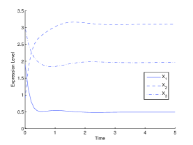
Figure 1: Trajectories of variables in S1.

IV-A2 Inferring Results of S2

The second benchmark system is a 4-D system where the parameters are listed in Tab.III. For initial conditions $X_{1}(0)=10$, $X_{2}(0)=1$,$X_{3}(0)=2$ and $X_{4}(0)=3$, data are sampled from time 0 to 5 with stepsize 0.1, and the time-course curves are illustrated in Fig.2 [10]. Compared with results presented in [10], the precisions of parameter values are a bit lower. However, we can obtained the correct network topology with 100% success rate except for the third equation. Considering that in [10] the initial parameter setting is generated by normal mutation performed on the known parameter values, we can conclude that our method is competitive to the method presented in [10] because we randomly generate initial parameters at the beginning.

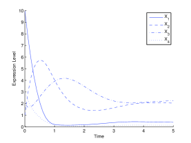
Figure 2: Trajectories of variables in S2.

TABLE III: Precise and Obtained Values for Parameters of Benchmark System S2.

$i$	$\alpha_{i}$	$g_{i1}$	$g_{i2}$	$g_{i3}$	$g_{i4}$	$\beta_{i}$	$h_{i1}$	$h_{i2}$	$h_{i3}$	$h_{i4}$	success rate
1	12	0	0	-0.8	0	10	0.5	0	0	0	100%
	(11.80,12.00)	(0.00,0.00)	(0.00,0.00)	(-0.79,-0.80)	(0.00,0.00)	(10.00,9.97)	(0.50,0.50)	(0.00,0.00)	(0.00,0.00)	(0.00,0.00)	-
1	8	0.5	0	0	0	3	0	0.75	0	0	100%
	(8.00,8.00)	(0.50,0.50)	(0.00,0.00)	(0.00,0.00)	(0.00,0.00)	(3.00,3.01)	(0.00,0.00)	(0.75,0.75)	(0.00,0.00)	(0.00,0.00)
3	3	0	0.75	0	0	5	0	0	0.5	0.2	90%
	(3.00,3.00)	(0.00,0.00)	(0.76,0.75)	(0.00,0.00)	(0.00,0.00)	(5.10,5.01)	(0.00,0.00)	(0.00,0.00)	(0.51,0.50)	(0.20,0.20)
4	2	0.5	0	0	0	6	0	0	0	0.8	100%
	(1.90,2.00)	(0.49,0.50)	(0.00,0.00)	(0.00,0.00)	(0.00,0.00)	(5.80,6.00)	(0.00,0.00)	(0.00,0.00)	(0.00,0.00)	(0.80,0.80)

IV-A3 Inferring Results of S3

The third benchmark system is a 5-D system where the parameters are listed in Tab.IV. For initial conditions $X_{1}(0)=10$, $X_{2}(0)=1$,$X_{3}(0)=2$, $X_{4}(0)=3$ and $X_{4}(0)=4$, data are sampled from time 0 to 10 with stepsize 0.1, and the time-course curves are illustrated in Fig.3 [10]. For this system, precisions of our obtained results are also lower than those reported in [10], especially for the second equation. This is because Liu et al. employed a local search procedure to refine the parameter values, while in our method no local searching process is implemented. Meanwhile, because derivatives of $X_{2}$ fluctuate in a small interval, our method only successfully obtain the correct connection of the second equation with success rate 85%.

TABLE IV: Precise and Obtained Values for Parameters of Benchmark System S3.

$i$	$\alpha_{i}$	$g_{i1}$	$g_{i2}$	$g_{i3}$	$g_{i4}$	$g_{i5}$	$\beta_{i}$	$h_{i1}$	$h_{i2}$	$h_{i3}$	$h_{i4}$	$h_{i5}$	success rate
1	2	0	0	0	0	0	2	0.5	0	0	0	-1	100%
	(1.99,2.00)	(0.00,0.00)	(0.00,0.00)	(0.00,0.00)	(0.00,0.00)	(0.00,0.00)	(1.99,2.00)	(0.50,0.50)	(0.00,0.00)	(0.00,0.00)	(0.00,0.00)	(-1.00,-1.00)
2	2	0.5	0	0	0	-1	4	0	0.5	0	0	0	10%
	(1.86,1.01)	(0.52,0.99)	(0.00,0.00)	(0.00,0.00)	(0.00,0.00)	(-1.03,-1.00)	(3.8351,4.03)	(0.00,0.00)	(0.52,0.50)	(0.00,0.00)	(0.00,0.00)	(0.00,0.00)
3	4(3.9)	0(0)	0.5(0.51)	0(0)	0(0)	0(0)	4(3.9)	0(0)	0(0)	0.8(0.81)	0(0)	0(0)	85%
	(3.93,4.00)	(0.00,0.00)	(0.51,0.50)	(0.00,0.00)	(0.00,0.00)	(0.00,0.00)	(3.93,4.00)	(0.00,0.00)	(0.00,0.00)	(0.81,0.80)	(0.00,0.00)	(0.00,0.00)
4	4	0	0	0.8	0	0	1	0	0	0	1	0	100%
	(3.97,4.00)	(0.00,0.00)	(0.00,0.00)	(0.81,0.80)	(0.00,0.00)	(0.00,0.00)	(0.98,1.00)	(0.00,0.00)	(0.00,0.00)	(0.00,0.00)	(1.01,1.00)	(0.00,0.00)
5	1	0	0	0	1	0	4	0	0	0	0	0.5	100%
	(0.98,1.00)	(0.00,0.00)	(0.00,0.00)	(0.00,0.00)	(1.00,1.00)	(0.00,0.00)	(3.97,4.00)	(0.00,0.00)	(0.00,0.00)	(0.00,0.00)	(0.00,0.00)	(0.50,0.50)

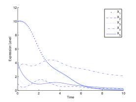
Figure 3: Trajectories of variables in S3.

IV-A4 Inferring Results of S4

The fourth benchmark system is a 5-D system where the parameters are listed in Tab.V[9]. To compare with the results reported in [9], we employ a data set of 60 samples generated from time 0 to 0.5 with stepsize 0.0083 with initial conditions $X_{1}(0)=0.7$, $X_{2}(0)=0.12$,$X_{3}(0)=0.14$, $X_{4}(0)=0.16$ and $X_{4}(0)=0.18$, and the time-course curves are illustrated in Fig.4. Results listed in Tab. V demonstrate that for equations 1, 2,and 5, the best obtained parameter values are more precise than what were reported in [9], however, inference results for equations 3 and 4 are not satisfactory. Fig. 4 illustrates that the curves of $X_{3}$ and $X_{4}$ rapidly reach equilibrium states after short increasing procedure, and consequently, our method, based on fitting of derivatives (slopes), could not identify the network connections well.

TABLE V: Precise and Obtained Values for Parameters of Benchmark System S4.

$i$	$\alpha_{i}$	$g_{i1}$	$g_{i2}$	$g_{i3}$	$g_{i4}$	$g_{i5}$	$\beta_{i}$	$h_{i1}$	$h_{i2}$	$h_{i3}$	$h_{i4}$	$h_{i5}$	success rate
1	5	0	0	1	0	-1	10	2	0	0	0	0	85%
	(4.91, 4.38)	(0.00, 0.00)	(0.00, 0.00)	(1.00, 1.43)	(0.00, 0.00)	(-1.01, -0.90)	(9.89, 9.57)	(2.02, 1.47)	(0.00, 0.00)	(0.00, 0.00)	(0.00, 0.00)	(0.00, 0.00)
2	10	2	0	0	0	0	10	0	2	0	0	0	100%
	(9.99, 9.32)	(2.00, 1.79)	(0.00, 0.00)	(0.00, 0.00)	(0.00, 0.00)	(0.00, 0.00)	(9.99, 10.56)	(0.00, 0.00)	(2.00, 2.06)	(0.00, 0.00)	(0.00, 0.00)	(0.00, 0.00)
3	10	0	-1	0	0	0	10	0	-1	2	0	0	10%
	(9.47, 10.88)	(0.00, 0.00)	(-1.05, -1.66)	(0.00, 0.00)	(0.00, 0.00)	(0.00, 0.00)	(9.49, 9.85)	(0.00, 0.00)	(-1.04, -1.25)	(1.84, 1.88)	(0.00, 0.00)	(0.00, 0.00)
4	8	0	0	2	0	-1	10	0	0	0	2	0	90%
	(22.37, 8.33)	(0.00, 0.00)	(0.00, 0.00)	(1.89, 1.90)	(0.00, 0.00)	(-0.54, -0.75)	(24.91, 9.89)	(0.00, 0.00)	(0.00, 0.00)	(0.00, 0.00)	(0.93, 2.24)	(0.00, 0.00)
5	10	0(0)	0	0	2	0	10	0	0	0	0	2	100%
	(9.92, 9.63)	(0.00, 0.00)	(0.00, 0.00)	(0.00, 0.00)	(2.06, 2.06)	(0.00, 0.00)	(9.89, 10.66)	(0.00, 0.00)	(0.00, 0.00)	(0.00, 0.00)	(0.00, 0.00)	(2.00, 2.14)

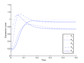
Figure 4: Trajectories of variables in S4.

IV-B Improving Inference Results by Multiple Data Sets

To improve the inference results of our method, we employ multiple data sets inferring the S-system S4. For comparison with results reported in [9], we generate four data set with initial conditions

1. $X_{1}(0)=0.7$, $X_{2}(0)=0.12$,$X_{3}(0)=0.14$, $X_{4}(0)=0.16$ and $X_{4}(0)=0.18$;

2. $X_{1}(0)=0.7$, $X_{2}(0)=0.12$, $X_{3}(0)=0.14$, $X_{4}(0)=0.16$ and $X_{4}(0)=0.18$;

3. $X_{1}(0)=0.1$, $X_{2}(0)=0.12$, $X_{3}(0)=0.7$, $X_{4}(0)=0.16$ and $X_{4}(0)=0.18$;

4. $X_{1}(0)=0.1$, $X_{2}(0)=0.12$,$X_{3}(0)=0.14$, $X_{4}(0)=0.16$ and $X_{4}(0)=0.7$,

where each data set contains 15 data samples. The obtained results are reported in Tab. VI.

TABLE VI: Improved Inference Results of Benchmark System S4 by Four Data Sets.

$i$	$\alpha_{i}$	$g_{i1}$	$g_{i2}$	$g_{i3}$	$g_{i4}$	$g_{i5}$	$\beta_{i}$	$h_{i1}$	$h_{i2}$	$h_{i3}$	$h_{i4}$	$h_{i5}$	success rate
1	5	0	0	1	0	-1	10	2	0	0	0	0	100%
	(4.84, 4.38)	(0.00, 0.00)	(0.00, 0.00)	(1.01, 1.43)	(0.00, 0.00)	(-1.05, -0.90)	(9.88, 9.57)	(2.03, 1.47)	(0.00, 0.00)	(0.00, 0.00)	(0.00, 0.00)	(0.00, 0.00)
2	10	2	0	0	0	0	10	0	2	0	0	0	100%
	(9.99, 9.32)	(2.00, 1.79)	(0.00, 0.00)	(0.00, 0.00)	(0.00, 0.00)	(0.00, 0.00)	(9.99, 10.56)	(0.00, 0.00)	(2.00, 2.06)	(0.00, 0.00)	(0.00, 0.00)	(0.00, 0.00)
3	10	0	-1	0	0	0	10	0	-1	2	0	0	100%
	(10.92, 10.88)	(0.00, 0.00)	(-1.00, -1.659)	(0.00, 0.00)	(0.00, 0.00)	(0.00, 0.00)	(10.92, 9.85)	(0.00, 0.00)	(-1.01, -1.25)	(1.67, 1.88)	(0.00, 0.00)	(0.00, 0.00)
4	8	0	0	2	0	-1	10	0	0	0	2	0	100%
	(8.66, 8.33)	(0.00, 0.00)	(0.00, 0.00)	(1.99, 1.90)	(0.00, 0.00)	(-0.97, -0.75)	(10.84, 9.89)	(0.00, 0.00)	(0.00, 0.00)	(0.00, 0.00)	(1.74, 2.24)	(0.00, 0.00)
5	10	0	0	0	2	0	10	0	0	0	0	2	100%
	(9.97, 9.63)	(0.00, 0.00)	(0.00, 0.00)	(0.00, 0.00)	(2.00, 2.06)	(0.00, 0.00)	(9.97, 10.66)	(0.00, 0.00)	(0.00, 0.00)	(0.00, 0.00)	(0.00, 0.00)	(2.01, 2.14)

By employing four data sets generated by different initial conditions, our method can perfectly identify the network topology of S4 with success rate 100%, and the obtained kinetic constant values are generally better than the results reported in [9]. However, sometimes rate constants obtained by our method are a bit worse than the compared results, because the rate constants are generated via the Least Square Method (LSM) in our method.

V Obtaining the GRN Settings from Candidate Non-dominated Solutions

Then, we select the Pareto solutions with minimum Akaike Information Criterion (AIC) value as the ultimate GRN inference results. The AIC for a candidate Pareto solution is computed as

$$AIC(\mathbf{x})=\log\left(\frac{1}{M}J_{i}(g_{i},h_{i})\right)+\frac{2(\|g_{i}\|+\|h_{i}\|)}{M},$$ (10)

where $M$ is the number of data samples [16]. Based on the results selected from obtained Pareto sets of 20 independent runs, we compute the sensitivity $S_{n}$ and specificity $S_{p}$ as follows:

$$S_{n}=\frac{TP}{TP+FN}$$ (11)

$$S_{p}=\frac{TN}{TN+FP}$$ (12)

where TP, FN, TN and FP represent the true positive (TP), false negative (FN), true negative (TN) and false positive (FP) predictions of the parameters. Average values of $S_{n}$ and $S_{p}$ for 20 independent runs for $S_{4}$ are listed in Tab. VII.

TABLE VII: Average Index Values of Inference Results of S4 Obtained by Four Data Sets.

i	TP	FN	TN	FP	$S_{n}$	$S_{p}$
1	3	0	6.95	0.05	$1$	0.99
2	2	0	8	0	$1$	1
3	3	0	6.6	0.4	1	0.94
4	3	0.05	6.1	0.85	0.98	0.88
5	2	0	8	0	1	1

It is shown that the sensitivity $S_{n}$ is equal to 1 except for the fourth equation ($S_{n}=0.98$), which means that for all equations the true network connections can be identified with a probability approximately equal to 1; however, sometimes the specificity $S_{n}$ is less than 1, which occurs when the true network topologies plus false positive connections can achieve better fitting errors.

VI Conclusion

In this paper, we presents an evolutionary multi-objective approach to inference network of S-system, using the SPEM decoupling the ODE system. Then, AIC is employed to select one Pareto solution as the final inference result. Due to the proposed multi-objective optimization model, there is no need to preset any parameter value before the inference MOEA is run. So, our method could be generally applicable to various kind of GRN model. However, we also find that this method is sensitive to the curve of expression level, and multiple data sets are needed to improve its performances. Future work will be focused on inference of GRN based on noisy data, and how to generalize the proposed method to infer big-scale GRNs.

References

- [1] M. I. Davidich and S. Bornholdt, “Boolean network model predicts cell cycle sequence of fission yeast,” PLOS One, vol. 3, no. 2, p. e1672, 2008.
- [2] N. Friedman, M. Linial, I. Nachman and D. Pe’er, “Using Bayesian networks to analyze expression data”, J. Computat. Biol., vol. 7, nos. 3-4, pp. 601-620, 2000.
- [3] A. V. Werhli, M. Grzegorczyk and D. Husmeier, “Comparative evaluation of reverse engineering gene regulatory networks with relevance network, graphical Gaussian models and Bayesian networks”, Bioinformatics, vol. 22, no. 20, p. 2523, 2006.
- [4] K. Y. Tsai and F. S. Wang, “Evolutionary optimization with data collocation for reverse engineering of biological networks”, Bioinformatics, vol. 21, no. 7, p. 1180, 2005.
- [5] W. Lee and Y. Hsiao, “Inferring gene regulatory networks using a hybrid GA-PSO approach with numerical constraints and network decomposition”, Inform. Sci., vol. 188, pp. 80-99, 2012.
- [6] Y. Li, S. Jin, L. Lei, Z. Pan and X. Zou, “Deciphering deterioration mechanisms of complex diseases based on the construction of dynamic networks and systems analysis”, Sci. Rep., vol. 5, e9283, 2015.
- [7] X. Xiao, W. Zhang and X. Zou, “A new asynchronous parallel algorithm for inferring large-scale gene regulatory networks”, Plos One, vol. 10, no. 3, p. e0119294, 2015.
- [8] D. Tominaga, N. Koga, and M. Okamoto, “Efficient numerical optimization algorithm based on genetic algorithm for inverse problem,” in Proc. Genet. Evol. Computat. Conf., vol. 251. 2000, p. 258.
- [9] L. Palafox, N. Noman, and H. Iba, “Reverse engineering of gene regulatory networks using dissipative particle swarm optimization“, IEEE Trans. Evol. Comp., vol. 17, no. 4, 577-587.
- [10] L. Liu, F. Wu, and W. Zhang , “Inference of Biological S-system Using Separable Estimation Method and Genetic Algorithm”, IEEE/ACM Trans. on Comput. Bio. Bioinform., vol. 9 no. 4: 955-965, 2012.
- [11] C. Spieth, F. Streichert, N. Speer and A. Zell, “Multi-objective model optimization for inferring gene regulatory networks”, in Proc. Evol. Mult.-Criter. Opt. Conf., vol. 3410, 2005, pp. 607-620.
- [12] P. Liu and F. Wang, “Inference of biochemical network models in s-sytem using multi-objective optimization approach”, Bioinformatics, vol. 31, no. 23, pp. 1085-1092, 2006.
- [13] P. Koduru, Z. Dong, S. Das, S. M. Welch, J. L. Roe and E. Charbit, “A multiobjective evolutionary-simplex hybrid approach for the optimization of differential equation models of gene networks”, IEEE Trans. Evol. Comp., vol. 12, no. 3, pp. 572-590, 2008.
- [14] X. Cai, Z. Hu, S. Das and S. M. Welch, “A hierarchical Pareto dominance based multi-objective approach for the optimization of gene regulatory network models”, in Proc. Evol. Comput. Conf., 2012, pp. 1-6.
- [15] Y. Chen, W. Xie and X. Zou, “A binary differetial evolution algorithm learning from explored solutions”, Neurocom., vol. 149, 1038-1047, 2015.
- [16] C. .W. Yao B. D. Hsu and B. .S. Chen, “Constructing gene regulatory networks for long term photosynthetic light acclimation in Arabidopsis thaliana”, BMC Bioinform., vol. 12, e335, 2011.