Using Wilson flow to study the SU(3) deconfinement transition

Abstract

We explore the use of Wilson flow to study the deconfinement transition in SU(3) gauge theory. We use the flowed Polyakov loop as a renormalized order parameter for the transition, and use it to renormalize the Polyakov loop. We also study the flow properties of the electric and magnetic gluon condensates, and demonstrate that the difference of the flowed operators shows rapid change across the transition point.

I Introduction

Wilson flow is a powerful new technique for the study of non-Abelian gauge theories main ; neuberger . It has been used for setting the scale in lattice computations main ; bmw ; staggered ; scale ; milc . It can also be applied in the construction of renormalized composite operators, like the energy-momentum tensor suzuki ; dpr and fermion bilinears chiral ; endo ; luscher . One example of the use of operators renormalized this way is the recent attempt to extract the renormalized pressure and energy density at finite temperature, $T$, in SU(3) gauge theory flowqcd . In this paper we use Wilson flow to create an order parameter for the finite temperature transition in the SU(3) pure gauge theory, and to examine gluon condensates for $T>0$.

The Wilson flow equation

$$\frac{dU_{\mu}(x,t)}{dt}\ =\ -\,\partial_{x,\mu}S[U]\,\cdot\,U_{\mu}(x,t),$$ (1)

produces a smeared configuration, $U_{\mu}(x,t)$, at any “flow time” t, given the initial condition $U_{\mu}(x,0)=U_{\mu}(x)$. Here $U_{\mu}(x)$ is the bare link ($x$ denotes a point in the 4-d Euclidean space-time lattice, and $\mu$ denotes one of the 4 directions), $\frac{\textstyle 1}{\textstyle g_{0}^{2}}S[U]$ is the action, and the derivative is a Hermitian traceless matrix. In this paper we will use the Wilson action, and our convention will be that

$$S[U]=\sum_{p}{\rm Re}\ \mathrm{Tr}\;\left[1-U(p)\right].$$ (2)

Here the plaquette operator, $U(p)$, is the ordered product of link matrices around a plaquette, and the sum is over all oriented plaquettes; $\partial_{x,\mu}\,S[U]$ in Eq. (1) is the traceless Hermitian matrix constructed from $U(p)$, the plaquette $p$ containing the link $(x,\mu)$.

Since the flow defined by Eq. (1) is diffusive, the smeared link operator has size which is proportional to $\sqrt{t}$. If one could choose to work at a flow time $t$, fixed in physical units while changing the lattice spacing, then the fat-link operators $U_{\mu}(x,t)$ would all be evolved to the same physical scale, and one would be able to construct renormalized composite operators from them. We explore such a construction for the Wilson line here.

A common way to define the scale is through the gluon condensate main :

$${\mathcal{E}}(t)=t^{2}{\bf E}(t),\qquad{\rm where}\qquad{\bf E}(t)=-\frac{1}{2}\overline{\mathrm{Tr}\;G_{\mu\nu}(x,t)G_{\mu\nu}(x,t)}.$$ (3)

$G_{\mu\nu}$ is the lattice version of the field strength tensor, and an average over the 4-volume of the lattice is denoted by the bar. One selects a value of $c$ and solves the equation

$$\langle{\mathcal{E}}(t)\rangle=c$$ (4)

for $t$. We will denote such choices of $t$ by $t_{c}$. The specific choice $c$ = 0.3 defines the flow time $t_{0.3}$, which is commonly called $t_{0}$ main . Another suggestion has been to use a derivative of $\mathcal{E}(t)$ bmw . Systematics of these scale setting schemes have been studied in detail scale ; staggered ; milc .

$\langle\mathcal{E}\rangle$ has widely been used for scale setting purposes in lattice QCD. In perturbation theory

$$\langle\mathcal{E}\rangle\ =\ \frac{3}{16\pi^{2}}\;g^{2}\left(1+c_{1}g^{2}+\mathcal{O}(g^{4})\right)$$ (5)

where, for pure gauge SU(3), $c_{1}=\frac{\textstyle 1.0978}{\textstyle 4\pi}$ when $g^{2}\equiv g^{2}_{\overline{\scriptscriptstyle{MS}}}(\mu=1/\sqrt{8t})$ main . One can also use $\langle\mathcal{E}\rangle$ to define a new coupling scheme,

$$g^{2}_{\rm flow}(t)\ =\ \frac{16\pi^{2}}{3}\langle\mathcal{E}\rangle.$$ (6)

In this paper we investigate the flow of two quantities which are very sensitive to the deconfinement transition. First, we look at the Polyakov loop, which is the order parameter for the deconfinement transition, but is highly singular as one takes the continuum limit. We discuss in the next section the use of flow to construct a continuum order parameter. Renormalization of the Polyakov loop using Wilson flow has also been considered in Ref. petreczky , which considered Polyakov loops in various representations, though we take a somewhat different approach to renormalizing them than what was done there. In the following section, we discuss the flow-time behavior of the gluon condensate and related observables. The gluon condensate is related to the nonperturbative nature of the QCD vacuum. As one crosses the deconfinement temperature $T_{c}$, the gluon condensate starts to melt. Also the electric and magnetic components of the gluon condensate show different temperature dependences. We will see that flow enhances the sensitivity of the gluon condensate to the onset of the transition.

In order to reduce the dependence of observables on the ultraviolet scale $1/a$, one should choose $c$ such that $a\ll\sqrt{t}$. At finite temperature, $T$, there is also an infrared scale proportional to $T$, and one should ideally choose

$$T\ll\frac{1}{\sqrt{t}}\ll\frac{1}{a}.$$ (7)

Since one also has $TN_{t}=1/a$, one sees that the hierarchies imply $1/N_{t}\ll\sqrt{t}T\ll 1$. With current day lattice $N_{t}\leq 16$, so the practical interpretation of “much less than” is no better than a factor of 4. As a practical example, when one chooses $c=0.3$, so that the flow scale is $t_{0}$, then $T_{c}\sqrt{t_{0}}\approx$ 0.25 in pure SU(3) gauge theory tct0 . Also, in most computations today, $\sqrt{t_{0}}/a\lesssim 2$. The process of scanning in $T$ while keeping $1/\sqrt{t}$ fixed (by fixing $c$) means that the hierarchy in Eq. (7) can be preserved only for $1/(N_{t}\sqrt{t})\ll T\ll 1/\sqrt{t}$. The suggestion in Ref. flowqcd , that one could keep $\sqrt{t}T=b$ fixed as one changes $T$ obviously has the limits $1/N_{t}\ll b\ll 1$. We study these questions here as part of our study of the renormalized Polyakov loop and gluon condensates at finite temperature.

II Polyakov loop

The deconfinement transition is associated with the breaking of the $Z_{3}$ center symmetry for SU(3) gauge theory. The Polyakov loop,

$$L(T,a)\ =\ \frac{1}{3V}\ \sum_{\bf x}\ \mathrm{Tr}\;\prod_{x_{4}=1}^{N_{t}}U_{t}(x)$$ (8)

transforms nontrivially under the $Z_{3}$ symmetry and acts as an order parameter for the transition. Here $x=({\bf x},x_{4})$ are the coordinates of the lattice sites, $U_{4}(x)$ are the link elements at site $x$ in the Euclidean time direction, $a$ is the lattice spacing, $N_{t}$ is the number of sites in the Euclidean time direction, the temperature, $T=1/(aN_{t})$, and the volume $V=N_{s}^{3}$ where $N_{s}$ is the number of sites in the spatial directions.

$\langle L(T,a)\rangle_{\scriptscriptstyle T}=0$ for temperature $T<T_{c}$, where the center symmetry is unbroken. Here $\langle\cdot\cdot\rangle_{\scriptscriptstyle T}$ denotes thermal averaging. For $T>T_{c}$ the $Z_{3}$ symmetry is spontaneously broken, and $\langle L(T,a)\rangle_{\scriptscriptstyle T}$ becomes nonzero. At finite volume, tunnelling between the $Z_{3}$ vacua make $\langle L(T,a)\rangle_{\scriptscriptstyle T}\to 0$ even in deconfiment phase; so we follow the standard practice of studying

$$P(T,a)\ =\ \langle|L(T,a)|\rangle_{\scriptscriptstyle T}.$$ (9)

$P$ is nonzero below $T_{c}$, $P|_{\scriptscriptstyle T<T_{c}}\sim\frac{\textstyle 1}{\textstyle V}$.

The bare Polyakov loop, as defined in Eq. (9), depends strongly on the lattice spacing $a$ polyakov :

$$P(T,a)\ =\ e^{-f(g^{2}(a))/aT}\ P_{\rm ren}(T).$$ (10)

Therefore $P(T,a)\to 0$ as $a\to 0$ and needs to be renormalized. Various techniques for renormalizing the Polyakov loop have been proposed in the literature renpol ; renpol1 . The renormalized Polyakov loop has also been calculated to next-to-leading-order in perturbation theory mikko ; in the $\overline{\rm MS}$ scheme,

$$\log P^{\overline{\scriptscriptstyle{MS}}}(T)=1+\frac{g^{2}C_{f}m_{\scriptscriptstyle E}}{8\pi T}+\frac{3g^{4}C_{f}}{16\pi^{2}}\left(\log\frac{m_{\scriptscriptstyle E}}{T}+\frac{1}{4}\right)+.....$$ (11)

where $g^{2}$ is the coupling in $\overline{\rm MS}$ scheme at a scale $\sim 4T$ and $m_{E}$ is the electric screening mass. For SU(3) gauge theory, $m_{E}=gT$ in leading order of perturbation theory.

II.1 Flowed Polyakov Loop

Wilson flow can be used to define an order parameter that is only mildly dependent on the lattice spacing $a$, and has a finite continuum limit: if we flow to a physical scale $t$, and define a Polyakov loop, $P(T,t,a)$ through Eq. (8) with the links replaced by flowed links, then $P(T,t,a)=P(T,t)+\mathcal{O}(a^{2}/t)$. Since the Wilson flow preserves center symmetry, the flowed Polyakov loop $P(T,t,a)$ acts as an order parameter for the deconfinement transition.

As discussed in Sec. I, if we flow the fields to time $t$, operators constructed out of the flowed fields are smeared to a radius $\sim\ \sqrt{8t}$. So we expect finite $a$ corrections to be small for $\sqrt{8t}\gg a$. On the other hand, for thermal physics we require the smearing radius $\sqrt{8t}\ll 1/T$. A window of $t$ satisfying both conditions can be obtained for the kind of lattices commonly used for finite temperature physics flowqcd .

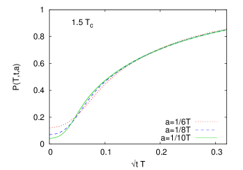
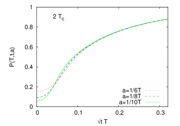
In Fig. 1, we show the flowed Polyakov loop for three different lattice spacings, corresponding to $N_{t}$ =6, 8 and 10, respectively, at two different temperatures. At $t=0$ we see the strong $a$ dependence indicated by Eq. (10). We see that this divergence is removed at fairly early flow times, $\sqrt{t}T\simeq 0.05$. The remaining finite $a$ corrections are suppressed when the flow time increases to $\sqrt{t}T\simeq 0.16$. If one does not include the $N_{t}$ = 6 data, then the figure shows that this happens at $\sqrt{t}T\simeq 0.12$. These flow times saturate the lower bound $b>1/N_{t}$, and correspond to $\sqrt{t}/a\simeq 1$ on the respective lattices. This is good as a practical matter, since it implies that the “much less than” in Eq. (7) can be replaced by “less than”.

Figure 1: Flowed Polyakov loop at 1.5 $T_{c}$ (left) and 2 $T_{c}$ (right). The thickness of the lines represent the $1\sigma$ bands.

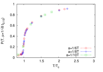
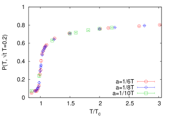
In Fig. 2 we explore the temperature dependence of the flowed Polyakov loop, $P(T,t,a)$, at three different lattice spacings, where the flow time is fixed to $t_{0.15}$ (left) and to $t=1/(5T)^{2}$ (right). As discussed in Appendix A the critical temperature is obtained from the peak of the susceptibility of the bare Polyakov loop, while $T/T_{c}$ is obtained using the flow scale. Since flowing to a fixed length scale like $t_{0.15}$ interferes with thermal physics at sufficiently high temperatures, in the left panel above we had to stop at a temperature $<1/\sqrt{8t_{0.15}}$. We note that $\sqrt{t}/a$ is large enough that the difference between the flowed loops at different $a$ are too small to be seen, for both these choices of $t$. Whenever our choice of flow time allows us to do this, we will suppress the argument $a$ and refer to $P(T,t)$.

This $a$-independent flowed Polyakov loop is sufficient to measure the continuum deconfinement transition in pure gauge theory. In the lower panels of Fig. 2, we show the susceptibility density

$$\chi_{\scriptscriptstyle P}(T,t)=\langle|P(T,t)|^{2}\rangle_{\scriptscriptstyle T}-\langle|P(T,t)|\rangle_{\scriptscriptstyle T}^{2}.$$ (12)

Since SU(3) gauge theory has a first order transition, $\chi_{\scriptscriptstyle P}(T,t)$ is expected to show a peak at $T_{c}$, just like the susceptibility for the non-flowed loop. Unlike the latter, however, the flowed susceptibility peak height does not change with $a$. The susceptibility $V\chi_{\scriptscriptstyle P}$ is known to scale like volume at $T_{c}$; since this volume scaling is caused by the two-peak nature of $P$ at the transition point, one expects a similar scaling to hold here. We do not explicitly check this volume dependence here.

Figure 2: The flowed Polyakov loop, $P(T,t,a)$, and its susceptibility density, $\chi_{\scriptscriptstyle P}(T,t,a)$, at fixed $t_{0}$ (left) and at fixed $\sqrt{t}T$ (right). The dependence on $a$ is too small to be extracted from these measurements. The thermal transition is identified correctly by both measures as one can see from the fact that the peak of the susceptibilities coincides with the $T_{c}$ measurement using the bare Polyakov loop.

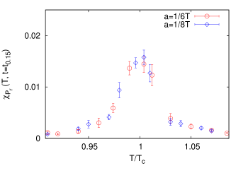
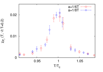
The symmetries of the Polyakov loop decide which screening masses can be seen in their correlations. Since the symmetries of the bare and flowed Polyakov loops are the same, they would give the same screening masses. The Polyakov loop correlations are sometimes used to determine the free energy of an infinitely heavy colour source placed in the gluonic medium. Determining this would require a renormalized Polyakov loop,whose extraction from data we turn to next.

II.2 Renormalized Polyakov loop

For gauge links flowed to a (sufficiently large) flow time $t$, fluctuations at scale $\gg 1/\sqrt{t}$ are strongly suppressed and the effective ultraviolet cutoff is $\sim 1/\sqrt{8t}$ main . Therefore, similar to Eq. (10) we can write

$$P(T,t)=e^{-\frac{R\left(g^{2}(t)\right)}{\sqrt{t}T}}\ P_{\rm ren}(T)$$ (13)

where $g^{2}(t)$ is the coupling evaluated at a scale $\mu\sim 1/\sqrt{8t}$. In leading order in $g$ (see Appendix B.1),

$$R\left(g^{2}(t)\right)=\frac{1}{3\pi^{2}}\frac{\sqrt{\pi}}{\sqrt{8}}\ g^{2}(t)\ \left(1+\mathcal{O}(g^{2})\right).$$ (14)

Following standard arguments polyakov ; dotsenko we expect that $\exp(R/\sqrt{t}T)P(T,t)\equiv P_{\rm ren}(T,t)$ is a function of temperature modulo $\mathcal{O}(\sqrt{t}T)$ corrections, and has a finite limit as $t\to 0$.

Figure 3: (Left)$P_{\rm ren}(T,t)$, Eq. (14) as function of flow time, at a temperature of 2 $T_{c}$ and different lattice spacings. Shown are the results using $g^{2}_{\overline{\scriptscriptstyle{MS}}}(\mu=1/\sqrt{8t})$ (solid lines, see below), $g^{2}_{\overline{\scriptscriptstyle{MS}}}(\mu=1/\sqrt{8t})$ extracted from $\bf E$ using Eq. (5) (dashed lines, denoted $g^{2}_{\scriptscriptstyle{\rm MS,flow}}$) and $g^{2}$ in the flow scheme(dotted lines). The thickness of the lines shows the error. (Right) $P_{\rm ren}(T,t)$ at a few temperatures on $N_{t}=8$ lattices. Here the two-loop $\overline{MS}$ coupling has been used. The two lines of the same style define the error band.

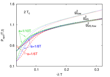
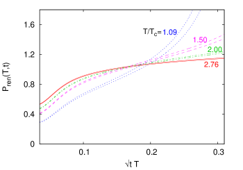
We first explore perturbative renormalization, using Eq. (14). The coupling $g^{2}_{\overline{\scriptscriptstyle{MS}}}(\mu=1/\sqrt{8t})$ is evaluated using the two-loop formula with $\Lambda^{n_{f}=0}_{\overline{\scriptscriptstyle{MS}}}\,=\,1.20(2)\;T_{c}$ largen , determined using plaquette values and two-loop perturbation theory. This value agrees, within error bars, with the value $1.24\pm 0.10$ quoted in Ref. tct0 and values in the range 1.18-1.22 obtained in Ref. flow2 , as well as an earlier measurement of $1.15\pm 0.05$ gupta . Note that the starting point of the calculation of $\Lambda^{n_{f}=0}_{\overline{\scriptscriptstyle{MS}}}$ is a lattice observable, and in the references cited above, two-loop perturbation theory was used to extract $\Lambda^{n_{f}=0}_{\overline{\scriptscriptstyle{MS}}}$; so it is only consistent to calculate the coupling using the two-loop formula.

In the left panel of Fig. 3 we illustrate the perturbative renormalization by showing $P_{\rm ren}(T,t)$ at 2 $T_{c}$ at different lattice spacings. One clear lesson from this exercise is that when $b\lesssim 1/N_{t}$, the multiplicative renormalization does not work. This follows from our earlier observation that there remains an $\mathcal{O}(a^{2}/t)$ piece which breaks scaling. That this should be large seems reasonable when one remembers that at such values of $b$ one has $\sqrt{t}/a\lesssim 1$. In this region of flow time there is a rapid rise in the value of the renormalized Polyakov loop. A much milder dependence on $t$ is observed at larger $b$. In this figure we also make a comparison with calculations where the coupling is calculated differently, in particular, calculations where $g^{2}_{\overline{\scriptscriptstyle{MS}}}(\mu=1/\sqrt{8t})$ is obtained through Eq. (5) (this is denoted by $g^{2}_{\scriptscriptstyle{\rm MS,flow}}$ in the figure), and also where the renormalization factor is calculated with the flow coupling $g^{2}_{\rm flow}$ (Eq. (6)). In each case the thickness of the line shows the error bar, combining the statistical error in the data and the uncertainty in the coupling. The calculation in the flow scheme is seen to result in a stronger $t$ dependence. This may indicate that the higher order corrections are larger in the flow scheme . The results are very close (for $\sqrt{t}>a$) in the two calculations where $g^{2}_{\overline{\scriptscriptstyle{MS}}}(\mu=1/\sqrt{8t})$ is obtained from the two-loop perturbation theory using $\Lambda^{n_{f}=0}_{\overline{\scriptscriptstyle{MS}}}$ and where it is defined through Eq. (5). The coupling $g^{2}_{\scriptscriptstyle{\rm MS,flow}}$, obtained using Eq. (5) from data at non-zero $a$, will have finite lattice spacing effects, and will also differ from other two-loop evaluations of $g^{2}_{\overline{\scriptscriptstyle{MS}}}(\mu=1/\sqrt{8t})$ at $\mathcal{O}(g^{6})$. The agreement in Fig. 3 indicates that such effects are small at these couplings. As $T$ is lowered, the agreement at fixed $\sqrt{t}T$ becomes worse, as one would expect from the increase in coupling.

In the right panel of the same figure, we show the perturbatively evaluated $P_{\rm ren}(T,t)$ at different temperatures, for lattices with spacing $a=1/8T$. In this, and all the following figures where a perturbative coupling is used, the two-loop $\overline{\scriptstyle MS}$ coupling, calculated using $\Lambda^{n_{f}=0}_{\overline{\scriptscriptstyle{MS}}}\,=\,1.20(2)\;T_{c}$, has been used. The growth of the error band at lower temperatures is because of the increase in scale dependence of the two-loop coupling. The knee at $\sqrt{t}\sim a$ can be seen at the different temperatures. For $\sqrt{t}>a$, the dependence of $P_{\rm ren}(T,t)$ on flow time is mild at high temperatures, but less so at lower temperatures.

To illustrate the temperature dependence of $P_{\rm ren}(T,t)$, we show it in Fig. 4 at both $c=0.15$ and $b=0.2$. The remnant $t$ dependence of $P_{\rm ren}(T,t)$ is clear by comparing the two panels of the figure. The corresponding susceptibility densities are also shown in the figure. The value of $T_{c}$, defined by the susceptibility peak, is consistent between the computations using different flow times. However, the value of $\chi_{\scriptscriptstyle P}$ depends on the choice of $t$ and the scheme.

Figure 4: The renormalized flowed Polyakov loop $P_{\rm ren}(T,t)$ (top), at flow times $t_{0.15}$ (left) and $t=(0.2/T)^{2}$ (right), and the corresponding susceptibilities (bottom).

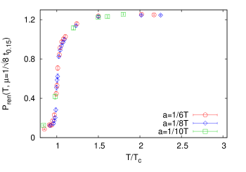
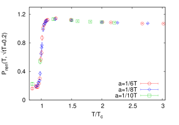
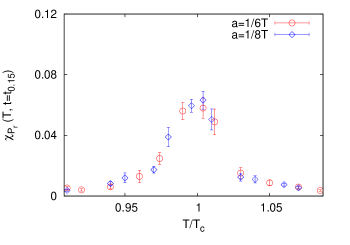
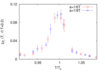
The substantial $t$ dependence in $P_{\rm ren}(T,t)$ defined through Eq. (14), in particular at lower temperatures, is not unexpected, as we are using only a leading order renormalization factor in perturbation theory. If one assumes that the $t$ dependence is due to remnant $\mathcal{O}(g^{4}\sqrt{t}T)$ effects, one can attempt a linear extrapolation of $P_{\rm ren}(T,t)$ to $t\to 0$. This is similar to the strategy of Ref. flowqcd . As Fig. 3 reveals, such an extrapolation is definitely not viable at smaller temperatures, where the $t$ dependence is strong and complicated. At higher temperatures, a linear behavior does not set in at $\sqrt{t}/a\sim 1$, but a linear extrapolation is feasible from a somewhat larger $t$. As an illustration of how the result of such a program will look, in the left panel of Fig. 5 we show the results of such an extrapolation. For definiteness, here we have chosen $\sqrt{t}T\in(0.2,0.3)$ for all the fits. This choice of range was guided by the discussion at the beginning of Section II.1, as well as a preference for a fixed range for all lattices, and the requirement that the result should not change, within errors, for a small change of the range.

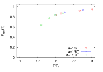
While the perturbative strategy is straightforward, as we have discussed, it may work only at high temperatures $\gtrsim 2T_{c}$. By going to higher $N_{t}$ it may be possible to make the extrapolation more stable at lower temperatures; however, it will be difficult to push it down to $T_{c}$ with realistic lattices. A more viable, nonperturbative strategy to calculate $P_{\rm ren}(T)$ at temperatures close to $T_{c}$ is to use the fact that the temperature dependence of the renormalization factor is simple, Eq. (13), and therefore, the renormalization factor at one temperature can be simply obtained from the renormalization factor at a different temperature modulo remnant linear $\sqrt{t}T$ corrections, which we expect to be small if we remain within our window $\sqrt{t}T\in(0.2,0.3)$. In order to extract $R\left(g^{2}(t)\right)$, we take a baseline value of the Polyakov loop at a given temperature. In what follows, we take the value $P_{\rm ren}(3T_{c})$ = 1.0169(1) renpol1 as the baseline. This determines $R\left(g^{2}(\sqrt{t}=1/10T_{c})\right)$, which can then be used to calculate $P_{\rm ren}$ to all temperatures up to 2 $T_{c}$. This process is then iterated to calculate $P_{\rm ren}$ at lower temperatures. This strategy is similar in spirit to that followed in Ref. renpol1 ; however, the use of flow makes the calculation simpler, as we do not need to match lattices at different lattice spacings to the same temperature. The renormalized Polyakov loop extracted this way is shown in the right panel of Fig. 5.

Figure 5: Renormalized Polyakov loop $P_{\rm ren}(T)$. (Left) Result of $t\to 0$ extrapolation of the leading order renormalized Polyakov loop, $P_{\rm ren}(T,t)$ (Eq. (14)). (Right) Renormalized Polyakov loop where the renormalization factor $R(g^{2}(t))$ is obtained from a nonperturbative matching; see text.

III Electric and magnetic condensate

The nonperturbative nature of the QCD vacuum is characterized by various condensates, which melt across the deconfinement transition. In the pure glue theory at zero temperature, $\bf E$, Eq. (3), is the only dimension four, scalar operator one can form. At finite temperatures Lorentz symmetry is broken, and two separate rotationally invariant, positive parity operators can be constructed out of $\bf E$:

$$E=\mathrm{Tr}\;G_{0i}G_{0i},\qquad M=\frac{1}{2}\mathrm{Tr}\;G_{ij}G_{ij}$$ (15)

which are related to the electric and magnetic gluon condensates, respectively. $O(4)$ symmetry at zero temperature implies $E$ and $M$ are not independent operators, and in the rest frame, $\langle E\rangle=\langle M\rangle=\frac{1}{2}\langle\bf E\rangle$.

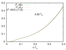
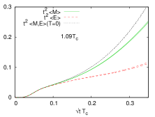
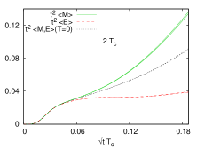
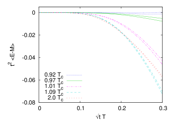
The flow behaviors of $E$ and $M$ turn out to be quite interesting. In Fig. 6 we show the dimensionless flowed quantities $t^{2}\langle E(T,t)\rangle$ and $t^{2}\langle M(T,t)\rangle$ immediately below and above $T_{c}$. In the same figures we also show the flow behavior of the same operator at $T=0$, studied on $N_{s}^{4}$ lattices at the same $a$. Below $T_{c}$ the flow time behavior of the operators is identical, indicating that even at $0.92T_{c}$, O(4) symmetry is approximately satisfied in the pure glue theory. In contrast, just above $T_{c}$, the flow behavior of $E$ and $M$ turn out to be very different from each other. While at small $t$, the flow behavior is influenced by the lattice cutoff and is similar to that seen for $\bf E$, at longer flowtime the growth of $\langle E(T,t)\rangle$ with flowtime flattens out while $\langle M(T,t)\rangle$ grows rapidly. Note that this behavior sets in in a very narrow region around $T_{c}$. While the breaking of the O(4) symmetry can already be seen at tree level, the interacting theory shows a much stronger effect (see Appendix B.2 and Fig. 10). This dynamical realization of the O(4) symmetry for all $T<T_{c}$, and its abrupt breaking just above, is consistent with the observation that both the energy density and the interaction measure vanish below $T_{c}$ and are finite just above. A similar realization of O(4) symmetry at finite temperature below $T_{c}$ was also observed in the screening of glueball-like operators glueball .

In Fig. 7 we show the difference $t^{2}\langle E(T,t)-M(T,t)\rangle$ . The panel on the left shows the flow-time behavior for different $T$. For $\sqrt{t}T\gtrsim 1/N_{t}$ this quantity is very sensitive to the deconfinement transition. For $T<T_{c}$ the quantity remains small. However, for $T>T_{c}$ significantly larger values are observed. Note that the $1/t^{2}$ singularity is cancelled between the electric and the magnetic operator expectation values. This allows us to study the difference $\langle E(T,t)-M(T,t)\rangle/T^{4}$.

Figure 7 shows $\langle E(T,t)-M(T,t)\rangle/T^{4}$ as a function of $T/T_{c}$. At $t=0$ this is a multiple of the entropy density, which is known to change abruptly across the pure gauge transition. At larger $t$ this jump is even more pronounced. What we would like to emphasize here is that for the flowed operator, this sharp jump arises from the flow behavior of $\langle E(T,t)\rangle$ and $\langle M(T,t)\rangle$. The flowed $\langle E-M\rangle/T^{4}$ can be used as an additional marker for the deconfinement transition.

Figure 6: The electric and magnetic condensate operators $t^{2}\langle M,E\rangle$ plotted against flow time, at temperatures of 0.92 $T_{c}$ (left), 1.09 $T_{c}$ (middle), and 2 $T_{c}$ (right), on lattices with $a=1/8T$. We show the $1\sigma$ band of the quantities. Also plotted are the zero temperature values of the same operators. In the left panel ($T<T_{c}$) the three bands almost completely overlap.

Figure 7: (Left) Flow time dependence of the operator $t^{2}\langle E-M\rangle$ at different temperatures, for lattices with $N_{t}=8$. The two lines of the same style define the 1 $\sigma$ band. (Right) Temperature dependence of the condensate difference $\langle E-M\rangle(T,t)/T^{4}$, without the flow and for two different flow times. Shown are the results for two different sets: the empty symbols correspond to $N_{t}=8$ lattices while the filled symbols correspond to $N_{t}=6$ lattices.

Connection to electric and magnetic gluon condensates

The vacuum gluon condensate is defined through the expression

$$\langle G^{2}\rangle=\left\langle\frac{8\beta(g)}{11g^{3}}\ \mathrm{Tr}\;G_{\mu\nu}G_{\mu\nu}(T=0)\right\rangle_{\rm subt}\ =\left\langle\frac{1}{2\pi^{2}}\,(1+\mathcal{O}(g^{2}))\,\mathrm{Tr}\;G_{\mu\nu}G_{\mu\nu}(T=0)\right\rangle_{\rm subt},$$ (16)

where $\beta(g)\,=\,\mu\frac{\textstyle\partial g}{\textstyle\partial\mu}\,=-b_{0}g^{3}-b_{1}g^{5}-...,\ \ b_{0}\ =\ \frac{\textstyle 11}{\textstyle 16\pi^{2}}.$ We have earlier used the quartic divergence of $\langle\bf E\rangle$ to define the flow scale. Here, the subscript on the vacuum expectation value (VEV) indicates that the hard mode contribution has been subtracted off. The resulting expectation value is finite and quantifies an important nonperturbative property of the vacuum svz .

Much effort has gone into the extraction of this property of QCD from either experiment or lattice calculations, but the extraction is still not stable. From analysis of the decay of the $\tau$ lepton, a value of 0.02-0.01 ${\rm GeV}^{4}$ has been quoted for the gluon condensate donoghue using a subtraction point $\sim(2\ \mathrm{GeV})^{4}$, while a recent determination quoted $0.009\pm 0.007\ \mathrm{GeV}^{4}$ ioffe . For SU(3) gauge theory a recent lattice determination quotes $\langle G^{2}\rangle=24.2\pm 8.0\ \Lambda_{\overline{MS}}^{4}$ bali , where $\langle G^{2}\rangle$ has been defined after subtraction of the perturbative part.

A finite temperature gluon condensate was defined analogously leutwyler by merely replacing the VEV in Eq. (16) by the thermal expectation value:

$$\langle G^{2}\rangle_{T}=\left\langle\frac{16\beta(g)}{11g^{3}}\ \bf E\right\rangle_{T,\rm subt}.$$ (17)

The complication of the hard mode subtraction can then be avoided by studying $\langle\underline{G^{2}}\rangle_{T}=\langle G^{2}\rangle_{T}-\langle G^{2}\rangle$. This difference is obtained simply from the difference of the expectation value of $\bf E$ on a thermal and a zero temperature lattice at the same $a$. $\langle\underline{G^{2}}\rangle_{T}$ is proportional to the trace of the energy-momentum tensor, and has been calculated from the plaquette operators for SU(3) su3thermo . In addition, we can also define the electric and magnetic gluon condensates, $\langle G_{\scriptstyle E}^{2}\rangle_{T}$ and $\langle G_{\scriptstyle M}^{2}\rangle_{T}$, analogously by replacing $\bf E$ by $E$ and $M$ respectively in Eq. (17) su3thermo . Finite temperature sum rule calculations use all these condensates lee .

The connection between the flowed condensate operators and the electric and magnetic gluon condensates can be extracted from Ref. suzuki :

$$\left.\begin{aligned} \langle\underline{G^{2}}\rangle_{T}\\ \langle\underline{G_{\scriptstyle E}^{2}}\rangle_{T}\\ \langle\underline{G_{\scriptstyle M}^{2}}\rangle_{T}\end{aligned}\right\}\ =\lim_{t\to 0}\ R(t)\cdot\left\{\begin{aligned} \langle\bf E(T,t)\rangle-\langle\bf E(T=0,t)\rangle\\ \langle E(T,t)\rangle-\langle E(T=0,t)\rangle\\ \langle M(T,t)\rangle-\langle M(T=0,t)\rangle\\ \end{aligned}\right.$$ (18)

where the renormalization constant $R(t)$ at leading order is

$$R(t)=\frac{1}{\pi^{2}}\ \left(1-2\,b_{0}\,\bar{s}_{2}\,g^{2}(\mu=1/\sqrt{8}t)\ +\ \mathcal{O}(g^{4})\right)$$ (19)

with $\bar{s}_{2}$ = 0.055785 suzuki .

Figure 8: The renormalized condensates $\langle\underline{G_{\scriptstyle E}^{2}}\rangle_{T}$ (left) and $\langle\underline{G_{\scriptstyle M}^{2}}\rangle_{T}$ (right) at $2T_{c}$, plotted as functions of flow time, at three different lattice spacings. The two lines of the same style define the error band.

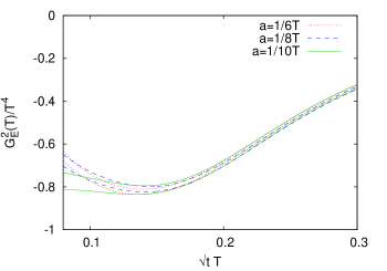
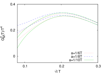
In Fig. 8 we show the renormalized condensates $\langle\underline{G_{\scriptstyle E}^{2}}\rangle_{T}$ and $\langle\underline{G_{\scriptstyle M}^{2}}\rangle_{T}$ as a function of flow time. Their sensitivity to the flow time means that the values of the renormalized condensates depend on the scale at which they are extracted. As we discussed before, the extraction of thermal physics from flowed configurations will require the flow time $\sqrt{t}T$ to be in a small window: $0.16\lesssim\sqrt{t}T\ll 1/\sqrt{8}\sim 0.35$. While the lattice spacing dependence is small within this window, neither a clear linear behavior, nor a prominent plateau can be seen for us to reliably extract the condensates using Eq. (18) . There is a hint of a plateau near the lower end of the window; in order to get a qualitative idea of the temperature dependence of the condensates, in Fig. 9 we show the renormalized condensates from this region, at the flow time $\sqrt{t}T=1/6$. As the discussion here suggests, this is to get only a qualitative idea of the dependence of the condensates on temperature.

Figure 9: (Left) The renormalized condensates $\langle\underline{G_{\scriptstyle E}^{2}}\rangle_{T}$ (open symbols) and $\langle\underline{G_{\scriptstyle M}^{2}}\rangle_{T}$ (filled symbols) plotted as a function of temperature, at flow time $\sqrt{t}T=1/6$. (Right) The corresponding plot for $\langle\underline{G^{2}}\rangle_{T}$.

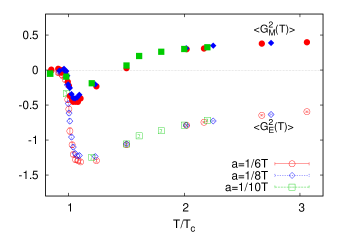
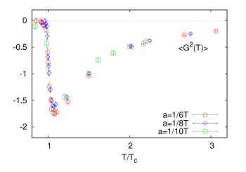
The figure shows some interesting features. Both $\langle\underline{G_{\scriptstyle E}^{2}}\rangle_{T}$ and $\langle\underline{G_{\scriptstyle M}^{2}}\rangle_{T}$ grow rapidly in magnitude just above the deconfinement transition, with $\langle\underline{G_{\scriptstyle E}^{2}}\rangle_{T}$ increasing more rapidly. The maxima of their magnitudes occur at approximately the same temperature, just above $T_{c}$. This leads to a sharp dip in $\langle\underline{G^{2}}\rangle_{T}$. After this temperature, the magnitude of both $\langle\underline{G_{\scriptstyle E}^{2}}\rangle_{T}$ and $\langle\underline{G_{\scriptstyle M}^{2}}\rangle_{T}$ decrease, while their difference is more stable. This causes the near-flat temperature dependence of $\langle E-M\rangle(T,t)$ seen in Fig. 7. Eventually $\langle\underline{G_{\scriptstyle M}^{2}}\rangle_{T}$ changes sign (see also Fig. 6). In the leading order, $\langle\underline{G_{\scriptstyle E}^{2}}\rangle_{T}$ = - $\langle\underline{G_{\scriptstyle M}^{2}}\rangle_{T}$ (Eq. (24)). An indication of the approach to such behavior is already seen in our highest temperatures. This leads to a very small value of $\langle\underline{G^{2}}\rangle_{T}$ at these temperatures, and therefore a very sharp drop after the peak just above $T_{c}$. Qualitatively, the behaviors are similar to that seen in Ref. su3thermo for analogous operators calculated from the plaquette, and renormalized using a nonperturbative $\beta$ function.

IV Discussion and conclusion

In this paper we have discussed the use of Wilson flow to study the deconfinement transition in SU(3) gauge theory. In particular, we have emphasized the construction of operators for studying the onset of the deconfinement transition. While the explicit computations done here are for the pure gauge theory, we expect the qualitative features to be true also for the theory with fermions. Therefore Wilson flow has the promise of being a powerful diagnostic tool for the deconfinement transition in QCD.

In Sec. II we have discussed flowed Polyakov loops, i.e., Polyakov loops constructed from links flowed to a fixed physical distance. Since the flow preserves Z(3) symmetry, and flowed Polyakov loops do not require renormalization, they give renormalized order parameters for the deconfinement transition. We have investigated both the cases of the flowed distance being fixed in terms of temperature or in terms of a temperature-independent physical length scale. Their behaviors are discussed in Sec. II.1 and shown in Fig. 2.

From the flowed Polyakov loops, renormalized (thin) Polyakov loops can be obtained. The renormalization using leading order perturbation theory, illustrated in Fig. 4, has remnant dependence on flow time, in particular close to the transition temperature. This is not entirely unexpected, as for the flow times we can use (which is restricted below by the lattice spacing $a$ of our lattices), the coupling is not small. We therefore turned to a nonperturbative renormalization. The results for the renormalized Polyakov loop are shown in Fig. 5. The use of the flow allowed us to conveniently do the nonperturbative matching involved in the renormalization. In principle, one can use the flow to do a purely perturbative renormalization also; the result of such a computation, with the leading order renormalization constant, is also shown. Perhaps not surprisingly, the perturbative method does not work very well especially as one comes down in temperature. Both higher order calculations and much finer lattices may be required for the perturbative approach to work near $T_{c}$.

Next we turn to a discussion of condensates of gluonic operators. At finite temperatures, two rotationally invariant, positive parity operators of dimension four can be constructed, corresponding to electric and magnetic gluon operators, Eq. (15). We find that their flow behaviors are very sensitive to the deconfinement transition: just around $T_{c}$ the flow behavior of the electric condensate changes drastically. As a result, the difference between the flowed operators acts as a marker of the transition. This is illustrated in Fig. 7.

An extraction of the renormalized gluon condensate from these results is difficult, because there is a dependence on flow time which is not cured by the leading order perturbative renormalization constant. Again it is not a surprise that leading order perturbation theory does not work at the lattices used by us. There is a hint of a mild plateau near the lower end of the window in flow time where thermal physics can be extracted. We use the results from this region to illustrate qualitative features of the thermal behavior of the renormalized gluon condensates in Fig. 9. The figure shows interesting thermal behavior of the electric and magnetic condensates, in particular just above the deconfinement transition.

Acknowledgements: This work was carried out under the umbrella of ILGTI. The computations reported here were performed on the gaggle cluster of the Department of Theoretical Physics, TIFR. We would like to thank Ajay Salve and Kapil Ghadiali for technical support, and Siddhartha Bhattacharyya, Anirban Lahiri and Shiraz Minwalla for discussions.

Appendix A Calculational details

For the results described in this paper, we calculated thermal and vacuum expectation values by generating zero and finite temperature lattices using a heatbath-overrelaxation algorithm. For the finte temperature runs, $N_{s}^{3}\times N_{t}$ lattices were generated with $N_{t}\ll N_{s}$. Thermal averaging requires the gauge fields to be periodic in the Euclidean time direction. We also imposed periodic boundary conditions in the spatial directions. At each value of the gauge coupling, we also performed a zero temperature run with $N_{s}^{4}$ lattices.

One Cabibo-Marinari pseudoheatbath step was followed by three overrelaxation steps; we call this combination a sweep. Autocorrelations get enhanced by Wilson flow milc ; staggered . To avoid autocorrelations, configurations were separated by a large number of sweeps: 500 sweeps for the finite temperature lattices and 200-500 sweeps for the zero temperature lattices. The Wilson action was used for the gauge fields. A complete list of the generated $T>0$ lattices is given in Table 1.

$24^{3}\times 6$			$32^{3}\times 8$			$32^{3}\times 10$
$\beta$	# conf	$T/T_{c}$	$\beta$	# conf	$T/T_{c}$	$\beta$	# conf	$T/T_{c}$
5.80	107	0.85	6.00	99	0.91	6.10	100	0.85
5.84	105	0.91	6.02	100	0.94	6.20	100	0.98
5.85	101	0.92	6.03	100	0.95	6.34	100	1.20
5.86	101	0.94	6.04	100	0.97	6.50	100	1.50
5.87	101	0.96	6.05	100	0.98	6.55	100	1.60
5.88	101	0.97	6.06	199	0.996	6.65	100	1.81
5.89	105	0.99	6.065	199	1.004	6.73	100	2.00
5.895	105	1.004	6.07	199	1.01	6.80	100	2.21
5.90	105	1.012	6.08	100	1.03
5.91	101	1.03	6.09	100	1.04
5.92	101	1.05	6.10	100	1.06
5.93	101	1.07	6.11	100	1.07
5.94	101	1.085	6.12	99	1.09
5.95	105	1.10	6.20	99	1.23
6.02	105	1.24	6.34	100	1.50
6.14	105	1.49	6.55	103	2.00
6.34	123	2.00	6.65	100	2.26
6.40	105	2.15	6.80	100	2.76
6.55	105	2.67
6.65	105	3.02

Table 1: List of finite temperature lattices generated for our calculations. Two configurations were separated by 500 x (1 HB + 3 OR) sweeps. For each finite temperature set on lattices $N_{s}^{3}\times N_{t}$, a set of $N_{s}^{4}$ lattices at the same $\beta$ was generated for the vacuum ensemble.

For generating the Wilson flow, the fourth order Runge Kutta was used main . See Ref. staggered for an analysis of the convergence of this scheme. We used $dt=0.01$ for our runs. For setting the temperature scales, the known results for $\beta_{c}$ at different $N_{t}$ were used, and $t_{0.12}$ was used for the relative scale at other $\beta$.

Appendix B Leading-order expressions

In the body of the paper we have referred several times to the behavior in leading order of perturbation theory. Here we write down the relevant expressions to this order for the Polyakov loop and the gluon condensates.

B.1 Polyakov loop

In leading order, the flowed Polyakov loop is given by

$$\log P(T,t) = -\frac{g^{2}}{4N_{c}}\,\int_{0}^{\beta}d\tau_{1}\,\int_{0}^{\beta}d\tau_{2}\,\langle B^{a}(\tau_{1},\vec{r})\,B^{a}(\tau_{2},\vec{r})\rangle$$ (20)

$$= -\frac{g^{2}}{4\pi^{2}}C_{f}\frac{\sqrt{\pi}}{\sqrt{8t}T}+\frac{g^{2}\,C_{f}\,m_{\scriptscriptstyle E}}{8\pi T}e^{z^{2}}\ \Phi_{c}(z)+\mathcal{O}(g^{4})$$

where $C_{f}=\frac{\textstyle N_{c}^{2}-1}{\textstyle 2N_{c}}$, $z=m_{\scriptscriptstyle E}\sqrt{2t}$, with the electric mass $m_{\scriptscriptstyle E}=gT$ for SU(3) gauge theory, and $\Phi_{c}(z)=\frac{\textstyle 2}{\textstyle\sqrt{\pi}}\int_{\scriptstyle z}^{\scriptstyle\infty}e^{\scriptstyle-x^{2}}dx$. Therefore

$$R\left(g^{2}(t)\right)=\frac{C_{f}}{4\pi^{2}}\frac{\sqrt{\pi}}{\sqrt{8}}\ g^{2}(t)\ \left(1+\mathcal{O}(g^{2})\right),\qquad\log P_{\rm ren}(T,t)=\frac{g^{2}(T)\,C_{f}\,m_{\scriptscriptstyle E}}{8\pi T}+\mathcal{O}\left(g^{4}(T),g^{4}\sqrt{t}T\right).$$ (21)

B.2 Gluon condensates

Insight into the flow behavior of the electric and magnetic condensates can be obtained by looking at their leading order expressions. Writing $\sqrt{t}T=x$, one gets, to $\mathcal{O}(g^{2})$,

$$\frac{<M>}{T^{4}} = \frac{4g^{2}}{\pi^{2}}\ \left(\sqrt{\frac{\pi}{2}}\frac{1}{8x^{3}}\,\Theta_{3}(0,e^{-8\pi^{2}x^{2}})\ -\ h(x)\right)+\mathcal{O}(g^{4})$$

$$\frac{<E>}{T^{4}} = \frac{4g^{2}}{\pi^{2}}\ \left(\sqrt{\frac{\pi}{2}}\frac{1}{16x^{3}}\,\Theta_{3}(0,e^{-8\pi^{2}x^{2}})+h(x)\right)+\mathcal{O}(g^{4})$$ (22)

$$h(x) = \sqrt{\frac{\pi}{2}}\frac{2\pi^{2}}{x}e^{-8\pi^{2}x^{2}}\,\Theta^{\prime}_{3}(0,e^{-8\pi^{2}x^{2}})-8\pi^{4}\sum_{n>0}n^{3}\,\Phi_{c}(2\sqrt{2}\pi xn)$$

where $\Theta_{3}(0,y)=\sum_{n}y^{n^{2}}$, $\Theta_{3}^{\prime}(0,y)=\frac{\textstyle d}{\textstyle dy}\Theta_{3}(0,y)$. From the above,

$$\frac{<E+M>}{T^{4}}=\frac{3g^{2}}{4\pi^{2}x^{3}}\sqrt{\frac{\pi}{2}}\Theta_{3}(0,e^{-8\pi^{2}x^{2}})+\mathcal{O}(g^{4}).$$ (23)

$\Theta_{3}(0,e^{-8\pi^{2}x^{2}})\sim\frac{\textstyle 1}{\textstyle\sqrt{8\pi}x}$ as $x\to 0$. Using this, as $T\to 0$ Eq. (23) reduces to the known leading order result $t^{2}<\mathcal{E}>=\lim_{T\to 0}x^{4}\frac{\textstyle<E+M>}{\textstyle T^{4}}=\frac{\textstyle 3g^{2}}{\textstyle 16\pi^{2}}$.

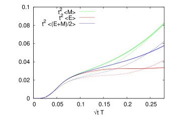
It is illustrative to compare the leading order expressions, Eq. (22), with data. Such a comparison is shown in Fig. 10. As the figure shows, the differential flow behavior of $E$ and $M$ is already seen in leading order; however, the behavior is much more pronounced in the full theory.

Figure 10: The finite temperature condensates $t^{2}<M,E>$ and their average, at 2 $T_{c}$, from our $N_{t}=8$ lattices (solid lines). Also shown, with dashed lines, are the corresponding leading order expressions, Eq. (22), Eq. (23).

Using Eq. (22) and Eq. (23) it is easy to calculate that for $t\to 0$,

$$\langle E(T)-E(T=0)\rangle\ =\langle M(T)-M(T=0)\rangle\ =-\frac{g^{2}\,(N^{2}-1)\,\pi^{2}}{30}\ T^{4}.$$ (24)

References

- (1) M. Lüscher, J. H. E. P. 1008 (2010) 071.
- (2) R. Narayanan and H. Neuberger, J. H. E. P. 0603 (2006) 064.
- (3) S. Borsanyi, et al., JHEP 1209 (2012) 010.
- (4) S. Datta, S. Gupta, A. Lahiri, A. Lytle and P. Majumdar, Phys. Rev. D 92 (2015) 094509 (arXiv:1507.00821).
- (5) See, e.g., R. Sommer, PoS LATTICE 2013 (2014) 015 (arXiv:1401.3270), and references therein.
- (6) A. Bazavov, et al., Phys. Rev. D 93 (2016) 094510 (arXiv:1503.02769).
- (7) H. Suzuki, Prog. Theor. Exp. Phys. (2013) 083B03; Prog. Theor. Exp. Phys. (2015) 103B03 (arXiv:1507.02360).
- (8) L. Del Debbio, A. Patella and A. Rago, J. H. E. P. 11 (2013) 212.
- (9) M. Luscher, J. H. E. P. 1304 (2013) 123.
- (10) T. Endo, K. Hieda, D. Miura and H. Suzuki, Prog. Theor. Exp. Phys. (2015) 053B03 (arXiv:1502.01809).
- (11) M. Luscher, PoS LATTICE2013 (2014) 016.
- (12) M. Asakawa, T. Hatsuda, E. Itou, M. Kitazawa and H. Suzuki, Phys. Rev. D90 (2014) 011501; Phys. Rev. D 92 (2015) 059902.
- (13) P. Petreczky and H.-P. Schadler, Phys. Rev. D 92 (2015) 094517 (arXiv:1509.07874).
- (14) A. Francis, O. Kaczmarek, M. Laine, T. Neuhaus and H. Ohno, Phys. Rev. D 91 (2015) 096002.
- (15) A.M. Polyakov, Nucl. Phys. B164 (1980) 171.
-
(16)
O. Kaczmarek, F. Karsch, P. Petreczky and F. Zantow,
Phys. Lett. B543 (2002) 41.
A. Dumitru, Y. Hatta, J. Lenaghan, K. Orginos and R.D. Pisarski, Phys. Rev. D 70 (2004) 034511. - (17) S. Gupta, K. Hübner and O. Kaczmarek, Phys. Rev. D 77 (2008) 034503.
- (18) Y. Burnier, M. Laine, M. Vepsäläinen, J. H. E. P. 0110 (2010) 054.
- (19) V.S. Dotsenko and S.N. Vergeles, Nucl. Phys. B 169 (1980) 527.
- (20) S. Datta and S. Gupta, Phys. Rev. D 80 (2009) 114504.
- (21) M. Asakawa, T. Iritani, M. Kitazawa and H. Suzuki, arXiv:1503.06516.
- (22) S. Gupta, Phys. Rev. D 64, 034507 (2001).
(23)
B. Grossman, S. Gupta, F. Karsch and U. Heller, Nucl. Phys. B 417 (1994) 289.
S. Datta and S. Gupta, Nucl. Phys. B 534 (1998) 392. - (24) M. Shifman, A. Vainshtein and V. Zakharov, Nucl. Phys. B 147 (1979) 385.
- (25) J.F. Donoghue and E. Golowich, Phys. Rev. D 49 (1994) 1513.
- (26) B. L. Ioffe and K.N. Zyablyuk, Eur. Phys. J. C 27 (2003) 229.
- (27) G. Bali, C. Bauer and A. Pineda, Phys. Rev. Lett. 113 (2014) 092001.
- (28) H. Leutwyler, in: Proc. Conf. QCD - 20 years later, eds. P.M. Zerwas and H.A. Kastrup (World Scientitic, 1993), 693.
- (29) G. Boyd, J. Engels, F. Karsch, E. Laermann, C. Legeland, M.Lütgemeier, B. Petersson, Nucl. Phys. B 469 (1996) 419.
(30)
R.J. Furnstahl, T. Hatsuda and S.H. Lee, Phys. Rev. D 42 (1990) 1744.
S. H. Lee and K. Morita, Mod. Phys. Lett. A 23 (2008) 2409.