Analyzing the Utility of a Support Pin in
Sequential Robotic Manipulation

Abstract

Pick-and-place regrasp is an important manipulation skill for a robot. It helps a robot accomplish tasks that cannot be achieved within a single grasp, due to constraints such as kinematics or collisions between the robot and the environment. Previous work on pick-and-place regrasp only leveraged flat surfaces for intermediate placements, and thus is limited in the capability to reorient an object.

In this paper, we extend the reorientation capability of a pick-and-place regrasp by adding a vertical pin on the working surface and using it as the intermediate location for regrasping. In particular, our method automatically computes the stable placements of an object leaning against a vertical pin, finds several force-closure grasps, generates a graph of regrasp actions, and searches for the regrasp sequence. To compare the regrasping performance with and without using pins, we evaluate the success rate and the length of regrasp sequences while performing tasks on various models. Experiments on reorientation and assembly tasks validate the benefit of using support pins for regrasping.

I Introduction

To rearrange and interact with a scene, a robot needs to be able to grasp and manipulate objects. One of the most common manipulation tasks is the pick-and-place, where the robot picks up a target object at an initial pose and then places it at a target pose. Sometimes the desired target pose is not reachable directly, due to the robot’s kinematics constraints or collisions between the robot and its surrounding environment. A typical solution is the pick-and-place regrasp, i.e., the robot uses a sequence of pick-ups and place-downs to incrementally change the object’s pose. In particular, after the object is picked up by the first grasp, it is stably placed in an intermediate location and then picked up again using another grasp. The relative pose between the object and the manipulator is fixed during each grasp, and only changes when the robot places the object down and regrasps it [1]. It is desirable if the object has many different ways of placements and each placement has many valid grasps, because this can provide the robot with more choices to incrementally adjust the object’s pose. More formally, the flexibility in placements helps to increase the connectivity of the regrasp graph [2] and is crucial for the quality of the resulting regrasp sequence.

There has been extensive work [3, 4] on pick-and-place regrasp since the 1980s, due to its importance for single arm manipulation. The majority of previous work assumed flat intermediate placement location, e.g., a horizontal ground or a tilted table, and focused on computing a feasible or optimal trajectory in the high-dimensional configuration space for achieving robotic pick-and-place tasks. However, since the convex hull of most objects only has limited number of faces, these objects can only be stably placed on a flat surface in a few different ways. This greatly limits the number of possible placements and thus also the connectivity of the resulting regrasp graph.

((a)) Pot lid organizer

((b)) Bicycle kickstand

Figure 1: The application of pin supports is popular in everyday life. Ikea’s pot lid organizer uses the pin support to stabilize the pot lids that are otherwise difficult to be placed. The bicycle kickstand is another example of support pin which helps to place a bike at a nearly vertical pose.

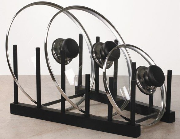
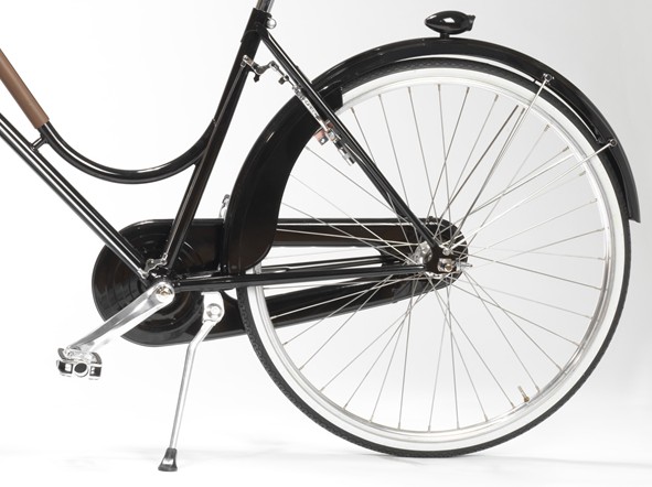
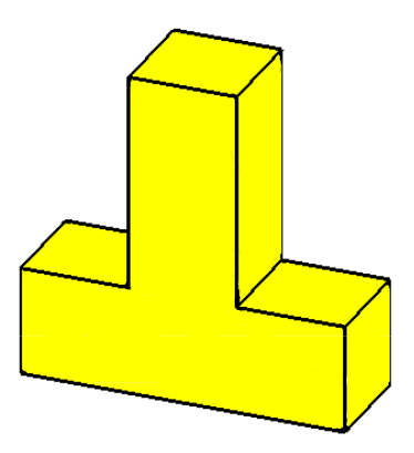
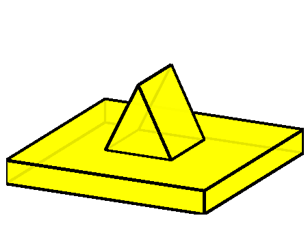
To address this challenge, in this paper we use an added pin for the intermediate placement, instead of only using a flat plane for support. This is motivated by real world examples of mechanisms that use pins to stabilize items that are otherwise difficult to orient on a flat surface, such as the pot lid organizer and the bicycle kickstand in Figure 1. The main advantage of a support pin lies in its ability to greatly increase the number of stable placements as well as the directions from which an object can be manipulated. Our previous work studying the use of a tiled surface for regrasping ([2, 5]) demonstrated the benefits of these two properties on the success rate of sequential robotic manipulation. Since a pin is able to provide more intermediate states and more candidate regrasps than those through usage of a tilted surface, we expect it to have better performance while planning the regrasping sequence. In particular, we choose one edge $e$ from the object’s convex hull, and one point $x$ from the surface of the object. Then a possible placement can be made by letting the object touch the pin at point $x$ and touch the flat surface at edge $e$ (refer to Figure 2(e)). All combinations of $e$ and $x$ correspond to the possible placements, which we then refine to yield valid stable placements through stability, collision, and friction tests. In this way, we can generate many more stable placements than when only using a flat plane support, and thus can greatly increase the connectivity of the regrasp graph. A support pin is also more beneficial for concave objects since it is able to use the concave part of the objects for the touch point $x$, while a flat plane would only be able to leverage the convex hull.

We perform statistical analysis on arbitrary mesh models with thousands of experiments to demonstrate the advantages of using support pins for regrasp. Our algorithm automatically computes the stable placements of an object on a support pin, finds force-closure grasps, generates a graph of regrasp actions, and searches for regrasp sequences. We use the two-layer regrasp graph in [2] to decouple the search of pick-and-place sequence and the search of grasps, and delay expensive inverse kinematics and collision detection computations until necessary. We evaluate the success rates of the tasks and the length of regrasp sequences with different mesh models, different pin lengths, and different tasks including reorientation (i.e., flipping) and assembly. For each task, the added pin is put in various locations relative to the robot, and the initial and goal poses of the objects are also randomized. Our results show that an added support pin is beneficial for all tasks. For some tasks involving pot lid like objects, which are difficult to be reoriented by a single manipulator through traditional regrasp sequence, the support pin can significantly increase the success rate of these tasks.

II Related Work

There has been extensive work on techniques related to grasp/regrasp, and of these the most relevant are the approaches to object placement planning and sequential robotic manipulation. Here we give a brief overview of these techniques.

II-A Object Placement Planning

Given an object and a placement area, object placement planning first needs to figure out the regions that are free for placement. This can be achieved either according to the environment geometry [6], or using a learning-based framework [7]. Among the computed free regions, the next step for object placement planning is to select a placement location that is suitable for the object, and to determine the object’s stable pose at that location. Most previous approaches only considered placement locations that are locally flat, and these locations are either pre-assigned [2, 5], or are selected online either autonomously [8] or interactively [6]. A few methods [9, 10] can leverage non-flat locations for placement. Jiang [9] outlined a learning-based framework to determine how to place novel objects in complex placement areas, while Baumgartl et al. [10] computed the geometric information of both the placement area and the object to determine whether a location is suitable for placement. Once the placement location is determined, the stable pose of the object at that location is computed by applying the contact constraint and the stability constraint [6, 10, 2]. Other constraints such as an orientation preference for man-made objects [11, 9] can also be taken into account by using the learning-based framework. After a placement has been planned, the robot needs to place the object accurately at the desired pose, which may be challenging in the real-world due to uncertainties. To deal with this problem, Kriegman [12] computed a so-called maximal capture region around the desired stable pose in the configuration space; if the object’s initial configuration is within the region, the object is guaranteed to converge to that pose under the force of gravity. Similar ideas were used by [13] to design the shape of the support surface.

In this paper, we focus on designing the placement area for maximizing the number of stable placements. In particular, we use a planar surface with one added pin as the placement area, and thus resulting in many more stable placements than when using only a flat surface or a surface with complex shapes.

II-B Sequential Robotic Manipulation

Solving manipulation problems requires planning a coordinated sequence of motions that involves picking and placing, as well as moving through the free space. Such sequential manipulation problem is challenging due to its high dimensionality. Early work in this area used an explicit graph search to find a sequence of regrasping motions [3]. Most recent approaches are constraint-based. They first formalize the geometric constraints being involved in the manipulation process, e.g., the object must be in a stable pose after being placed down, the relative pose between the manipulator and the object must be fixed during the grasp, and two objects should not collide with each other. Next, they compute a grasp sequence that can satisfy all these constraints. Some methods [14, 15] used these constraints to define a set of interconnected sub-manifolds in the task space, and then computed a solution sequence using probabilistic roadmaps embedded in the constrained space. Other approaches [16, 8, 17] used these constraints to represent sequential manipulation problems as constraint-satisfaction problem (CSP), and then solved the CSP using variants of the backtracking search.

In order to improve the manipulation flexibility, some recent work began to incorporate non-grasp polices in the manipulation. There are many prehensile or non-prehensile strategies besides grasping, such as non-prehensile pivoting [18] and prehensile pivoting [19], non-prehensile pushing [20] and prehensile pushing [21]. Regrasp policies leveraging external forces or external environments have also been proposed [22, 21] for in-hand manipulation. To make use of these non-grasp policies, Lee et al. [23] proposed the concept of extended transit, i.e., the transition motion will not only include the transitions between prehensile grasps, but also those between non-prehensile manipulation strategies. A similar idea was also proposed by [24], which used grasping and pushing for transition motion, but only used grasping for transfer motion.

Multi-arm grasping/regrasping is another active area in sequential robotic manipulation, where the difficulty lies in the high dimensional configuration space of the multi-arm system and the combinatorial complexity due to large number of regrasps and handoffs. Following the initial study by Koga et al. [25], sampling-based approaches [26] and grid based searches [27] were proposed for planning the manipulation sequence for a dual-arm robot. Both these methods have recently been extended to handle multi-arm manipulation problems [28, 29].

One well-known dilemma for the sequential manipulation is the size of the pre-defined grasp set: a large grasp set will make the planning algorithm too slow, but a small grasp set will result in a high failure rate. Previous approaches tend to use a grasp set with size smaller than 30, e.g., 15 in [26] and 12-14 in [29], and thus they usually are not robust for practical applications. To deal with this challenge, our previous work [2, 5] proposed a two-layer regrasp graph to leverage a large number of grasps efficiently. In this paper, we concentrate on generating motion sequences for pick-and-place regrasp using the regrasp graph proposed in [2, 5], which is applicable to complicated mesh models and large-scale experiments.

III Pick-and-place Regrasp using a Support Pin

In this section, we discuss the details about our pick-and-place regrasp leveraging a support pin for placement. Our method mainly consists of three parts: 1) computing all possible stable placements with collision-free grasps associated; 2) building a regrasp graph whose connectivity reflects the number of common grasps associated with each pair of different placements; 3) searching in the regrasp graph for a shortest path between the initial and goal placements, in order to generate a possible pick-and-place grasp sequence.

III-A Placement and Grasp Computation

We first discuss how to generate all possible placements and the associated grasps, given the mesh model of an object and the length of the support pin. This is the key problem when performing sequential robotic manipulation with a support pin, and has not been studied in contemporary literature.

Our method is based on the fact that any placement requires three linearly-independent pivot points. Since the support pin already provides one pivot point, the object itself only needs to provide another two, which correspond to one edge on the object’s convex hull. As a result, we compute placements by finding all combinations of a single edge on the convex hull and a single point on the object where the pin touches. Naturally, some of the edge-point pairs may not result in a valid placement due to collisions or instability, and thus we will need to filter out these invalid edge-point combinations. An overview of the entire pipeline for placement computation is shown in Figure 2, and we proceed with a detailed explanation of this pipeline.

Figure 2: The flowchart for computing all possible placements of an object on a support pin, as well as the grasps associated with each placement. Given an object in (a), we first compute its convex hull (b), and also perform uniform sampling on the surface of the object (c). Next, we find all combinations of convex hull edges and surface samples, and each pair of edge-sample will produce one edge-pin pair (d), which corresponds to a candidate placement. We only keep the candidate placements that have passed the stability checking and collision checking, and then transform them to the world coordinate system to obtain valid edge-pin placements (e). We also compute the total grasps for the object (f). Finally, for each placement, we filter out those grasps that are infeasible due to collision or torque limits, and obtain the valid grasps associated with each placement (g). These placements and associated grasps are then used to build a regrasp graph (h), which is used for the reorientation task in (i). The green edge $e$ in (d) (e) is one edge of the convex hull, and it makes a placement together with the pin $\overline{bx}$ in (e), where the point $x$ is one sample on the object surface and the point $b$ is the pin base on the support plane. The blue segments in (f) and (g) denote grasps, where the longer segments together with the shorter segments and their ends illustrate the approaching and opening directions of the grippers, respectively.

III-A1 Touching Point Sampling for the Support Pin

The support pin’s candidate touching points on the object are generated by sampling the mesh surface, as shown in Figure 2(c). To avoid missing important placement candidates, we want these samples to be evenly distributed over the object’s surface. To achieve this, we first perform principal component analysis on each face of the object’s mesh model to obtain two main axes for each face. Sample points denoted by $\{x\}$ are then generated uniformly along these two axes with a reasonable step size. Marginal points too close ($<5$mm in all our experiments) to the model’s face edges are removed after the sampling, since these points will not result in a reliable placement. In parallel, we also compute the convex hull of the object to obtain the candidate edge $e$ where the object touches the flat support plane, as shown by the green line in Figure 2(d).

III-A2 Finding Base Point of the Support Pin

Given a sample touching point $x$, and one edge $e=\overline{e_{1}e_{2}}$ on the convex hull, we need to determine whether the $(x,e)$ pair will make a valid placement on a pin with length $l$. If a valid placement exists, we need to then compute the orientation of the pin relative to the object. For this purpose, we first compute the distance from $x$ to a line passing through the endpoints $e_{1}$ and $e_{2}$. If such distance is shorter than $l$, then it is impossible to find a valid placement. Otherwise, we continue to find a point $b$ at which the pin touches the support plane and satisfies the following constraints:

$$\left\{\begin{array}[]{c}\|x-b\|=l\\ (x-b)\cdot(e_{1}-b)=0\\ (x-b)\cdot(e_{2}-b)=0\end{array}\right.$$ (4)

Solving these three equations yields two solutions for $b$, one of which can be easily discarded. The edge $e$ and the pin $\overline{bx}$ together form one candidate placement. We need to verify the validity of this candidate placement by checking whether it satisfies a set of constraints. First, the pin $\overline{bx}$ should not collide with the object. Second, this placement should be stable, i.e., the object’s center of mass should have a projection inside the triangle $\Delta e_{1}e_{2}b$. Finally, the angles between the pin direction and the touching face’s normal should be within a range determined by a given friction factor $\mu$, to make sure that the object will not slide over the pin. We only keep the candidate placements that satisfy all these constraints. For each convex hull edge, there may be more than one associated placement, and we choose the placements that result in the highest center of mass for the object. This is because for an object with uniform distribution of mass, a higher center of mass means that more space will be left for collision-free grasps, which increases the connectivity of the regrasp graph. The collection of all placements is denoted as $\mathbf{p}^{\text{pin}}=\{p_{1}^{\text{pin}},p_{2}^{\text{pin}},...\}$. In our experiment, we will also use the traditional placements only leveraging a planar surface as the support [2], which are denoted as $\mathbf{p}^{\text{planar}}$.

III-A3 Calculating Total Grasps

We then compute the set of total grasps, namely $G=\{g_{1},g_{2}....\}$, associated with the object without considering collision-free and inverse kinematics constraints. One example of the total grasps is shown in Figure 2(f). Each grasp $g_{i}$ is computed according to the algorithm in [2] such that it satisfies force-closure constraints and consists of the position and orientation of the robot hand. For the Robotiq 2-finger adaptive gripper that we used, the grasps are computed by first examining possible parallel face pairs on the object, and then sampling the rotation direction around normals of the parallel faces. We can adjust the number of sampled directions to control the grasp density. We will discuss the relationship between the grasp density and the success rates of the pick-and-place tasks in Section IV.

III-A4 Grasps Associated with Placements

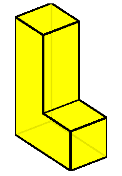
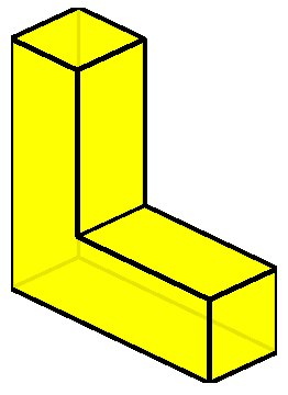
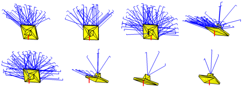
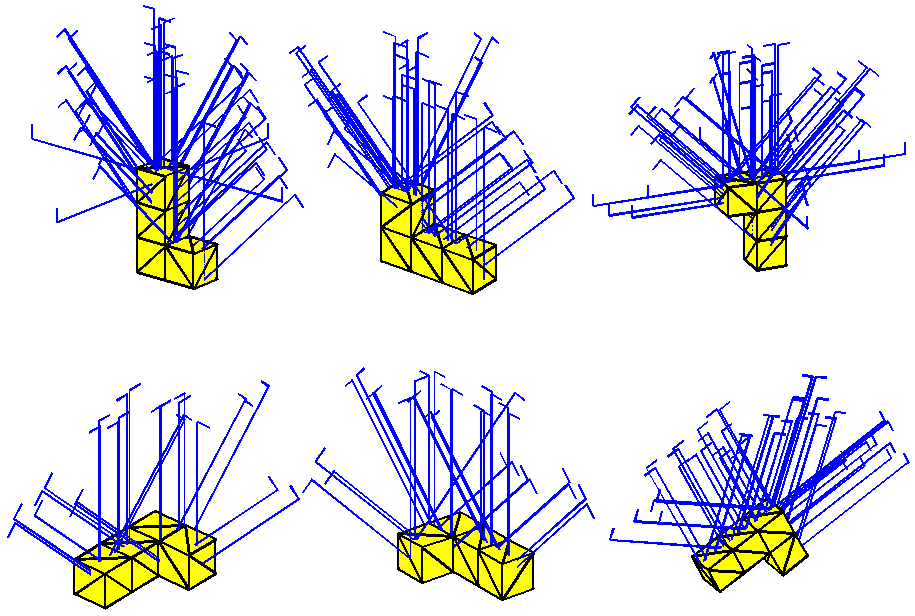
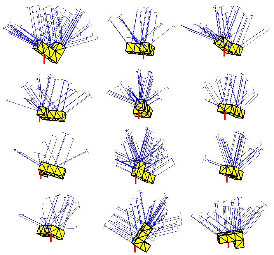
Possible grasps associated with a pin-based placement are found by transforming the total grasps from the object’s local coordinate to the current world frame of the placement, and then checking the collision between the gripper and the support pin, as well as the collision between the object and the flat support surface. After filtering out the invalid grasps, we obtain all valid grasps associated with a placement, and we denote the association as $\{p_{i},G^{i}\}$, where $p_{i}$ is a placement from either $\mathbf{p}^{\text{pin}}$ or $\mathbf{p}^{\text{planar}}$ and $G^{i}=\{g_{p}^{i},g_{q}^{i},...\}$ is the valid grasp set for $p_{i}$. In Figure 7(b), we show all the placements and associated grasps for one “L” shaped object (as shown in Figure LABEL:sub@fig:model:1t1p) using the support pin for placement. For comparison, we also use the method in [2] to compute the placements and grasps for the traditional regrasp of placing objects only on a flat surface, and the results are shown in Figure 7(a).

III-B Regrasp Graph Construction

Given the placements and the associated grasps, we build a two-layer regrasp graph where the first layer is composed of placements and the second layer is composed of grasps. The hierarchical structure of the regrasp graph can help to delay the computation for inverse kinematics and collision checking until necessary, and thus reduces the combinatorial complexity of the manipulation planning.

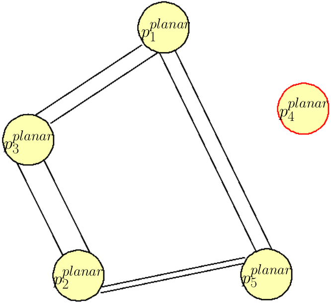
In the first layer, two placements $p_{i}$ and $p_{j}$ are connected by one edge if their associated grasp sets $G^{i}$ and $G^{j}$ are not disjoint, i.e., $G^{i}\cap G^{j}\neq\emptyset$. In the second layer, we add edges between grasps that are shared by two placements. For instance, given two connected placements $p_{i}$ and $p_{j}$, suppose the intersection of their associated grasp sets is $G^{i}\cap G^{j}=\{g_{u},g_{v},...\}$. Then we will add edges $(g_{u}^{i},g_{v}^{i})$, $(g_{u}^{j},g_{v}^{j})$, …, and $(g_{u}^{i},g_{u}^{j})$, $(g_{v}^{i},g_{v}^{j})$ in the second layer graph, where we use $g_{*}^{i}$ and $g_{*}^{j}$ to denote $g_{*}$’s corresponding grasps in $G_{i}$ and $G_{j}$, respectively. For more details about how to build this graph, please refer to [2]. Examples of the first layer of the regrasp graph are shown in Figure 2(h) and Figure 9.

III-C Grasp Sequence Computation

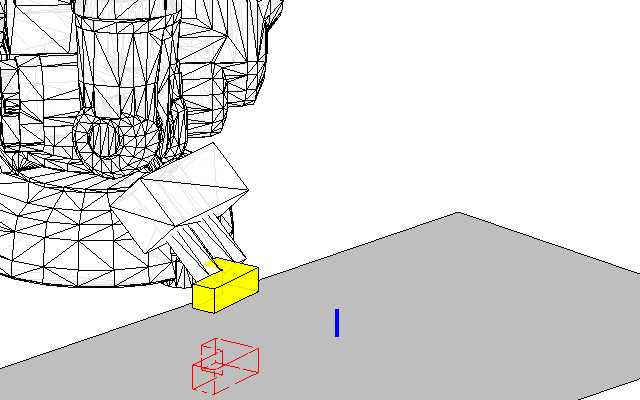
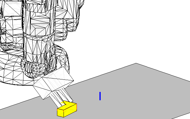
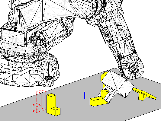
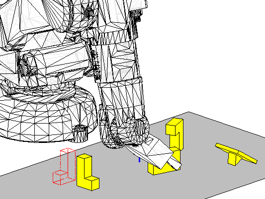
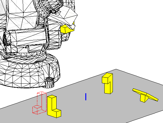
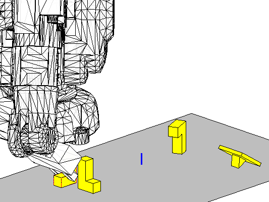
The motion sequence for manipulating the object to perform reorientation or assembly tasks can be generated by first searching in the first layer regrasp graph for a shortest path connecting the initial and goal placements (as shown by the $p_{\text{init}}^{\text{planar}}$ and $p_{\text{goal}}^{\text{planar}}$ in Figure 2(h)). Then in the second layer, by considering the connectivity between the grasps associated with the placements along the shortest path, a sequence of grasps can be generated. After that, we perform collision checking and solve for inverse kinematics at each pick-up and place-down moment. One example of the generated grasp sequence is shown in Figure 5.

IV Experiments and Analysis

In this section, we demonstrate the advantage of using an added support pin for intermediate placement in the pick-and-place regrasp. In particular, we perform a large number of reorientation tasks in a simulated environment. We compare the success rates and the lengths of the resulting regrasp sequences in the presence of two different placement settings: one only using the flat plane, and the other using an added support pin. Meanwhile, the effects of different grasp density and pin length are compared against the above two criteria. We also use the support pin placement to accomplish one assembly task which is not feasible while only using planar surface as support.

We implemented our algorithms in Matlab on an Intel Core i7 CPU running at 3.40GHz with 32GB of RAM and running Ubuntu 12.04 LTS. All the timing results are generated using a single core.

IV-A Experiment Settings

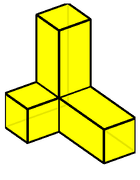
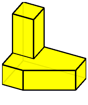
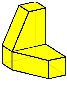
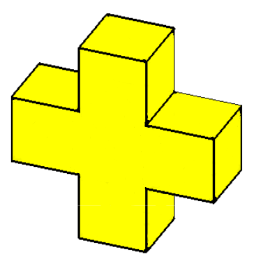
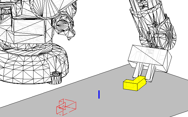
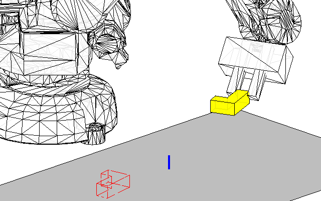
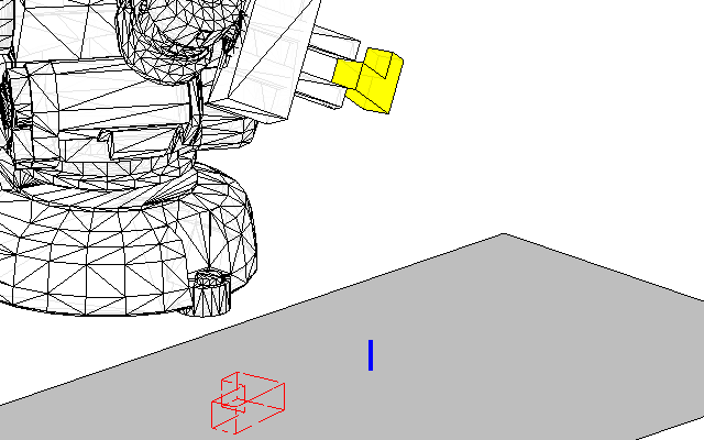
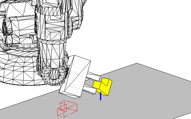
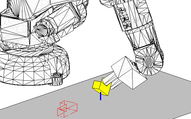
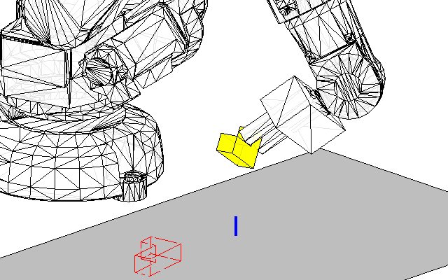
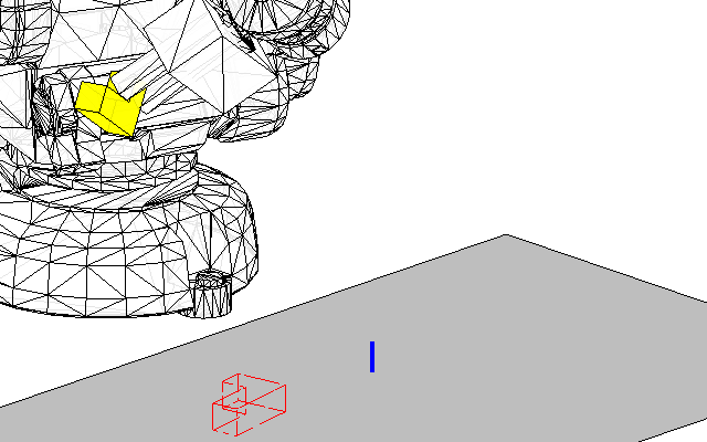
We use an ABB IRB140 robot manipulator with a 2-finger Robotiq gripper 85 mounted as the end-effector to repeatedly perform reorientation tasks for several different object models as illustrated in Figure 3. Among these object models, (a)-(e) form a morphing sequence where we increase the object’s volume by gradually adding more elements to the shape $l$. We select a $0.8$ by $0.6$ meter rectangular working area in front of the robot, as shown in Figure 4. This working area is evenly divided into a $20$ by $15$ grid of $4$ by $4$ cm grid squares. We let each corner of each grid square, $x_{\text{grid}}$, be the initial and goal positions for the object to be manipulated, while the initial and goal orientations are randomized. The object’s initial and goal placements are also randomly chosen from $\mathbf{p}^{\text{planar}}$, i.e., the beginning and end of the manipulation are always placements on the flat surface. For regrasp transitions, the object will be placed in an intermediate location which is $20$ cm to the left of $x_{\text{grid}}$ in order to avoid the collision between the pin and the object at initial and goal poses. Ten trials were performed for each corner of the grid square, and thus, in total, there are $(20+1)\times(16+1)\times 10=3360$ trials for each object. An example of the reorientation sequence is shown in Figure 5, where the robot uses one regrasp placing on the pin to successfully reorient one “L” shaped object. Unless otherwise stated, the length of the pin used in our experiment is $3$ cm, and the grasp density is $8$ directions.

((a)) $l$

((b)) $el$

((c)) $3t$

((d)) $3ts$

((e)) $3t2s$

((f)) $cross$

((g)) $t$

((h)) $1t1p$

Figure 3: Mesh models for all objects used in our experiments. All objects are non-convex, and $1t1p$ is an object of the pot lid shape. The first five objects (a)-(e) form a morphing sequence where we increase the object’s volume by gradually adding more elements to the shape $l$. The height of all objects from (a) - (g) is $9$ cm, and all objects can be bounded in a cube of size $9$ by $9$ by $9$ cm.

Figure 4: The experimental setting for the reorientation task. The $0.8$ by $0.6$ meter rectangular working area in front of an ABB IRB140 robot is evenly divided into a $20$ by $15$ grid of $4$ by $4$ cm grid squares.

((a))

((b))

((c))

((d))

((e))

((f))

((g))

((h))

((i))

((j))

((k))

((l))

Figure 5: The regrasp sequence for reorienting an “L” shaped non-convex model using one support pin as intermediate placement. The sequence is computed with the two-layer regrasp graph built on the grasps computed by sampling the mesh model. (f) and (g) are the transition steps while regrasps occur.

IV-B Comparison of Placements and Grasps

We first compare the cases with only planar support to the cases with an added support pin in terms of placements and associated grasps. In Figure 6 and Figure 7 we show the results for a pot lid like object $1t1p$ and for an “L” shaped object $l$.

The pot lid shape $1t1p$ has a large body and a small handle, and all stable placements for it could be roughly categorized into two scenarios: handle-down and body-down. While only using the planar surface as support, there are only five different placements as shown in Figure 6. Even worse is that the grasps associated with the body-down placements are limited only to the handle part and that there are very few of such grasps, as illustrated by the placement $p_{4}^{\text{planar}}$ in Figure 6(a). As a result, the connectivity is low in the corresponding regrasp graph and sometimes there may even be no connection between two placements as shown in Figure 9(a). With the help of a pin, we note an increase in interconnected placements added to the graph and also an increase in common grasps associated with different placements, as shown in Figure 6(b). This in turn increases the connectivity of the regrasp graph, as shown in Figure 9(b).

As shown in Figure 7, the “L” shaped object $l$ also has more stable placements while using the pin support, which helps to increase the connectivity of the resulting regrasp graph.

((a)) Placements and grasps with only a support plane

((b)) Placements and grasps with an added support pin

Figure 6: For the pot lid like object $1t1p$, we compare its placements and associated grasps between only using the planar surface as support and using an added support pin as the placement area.

((a)) Placements and grasps with only a support plane

((b)) Placements and grasps with an added support pin

Figure 7: For the “L” shaped object $l$, we compare its placements and associated grasps between only using the planar surface as support and using an added support pin as the placement area.

((a)) Placements and grasps with only a support plane

((b)) Placements and grasps with an added support pin

Figure 8: For the $cross$ model, we compare its placements and associated grasps between only using the planar surface as support and using an added support pin as the placement area.

((a))

((b))

Figure 9: The regrasp graphs of $1t1p$ for the planar placement and for the pin placement, respectively. (a) is the regrasp graph for planar placement, and $p^{\text{planar}}_{4}$ is the $4$-th body-down placement in Figure 6(a), and we can see it has no connection with other placements in the graph, and this suffers the connectivity of the entire graph. (b) is the regrasp graph for the pin placement, which has more placements than the planar support case. In addition, $p^{\text{pin}}_{5}$, $p^{\text{pin}}_{6}$, $p^{\text{pin}}_{7}$ and $p^{\text{pin}}_{8}$ correspond to the body-down placements in Figure 6(b), and they are well connected to the other placements thanks to the usage of the added support pin.

IV-C Comparison of Success Rates

We then compare the reorientation task’s success rates while using the pin and planar placement settings. From the result shown in Figure 10, we can see that the success rate of the pin placement is higher than that of the planar placements for all different objects except the $cross$ model. The advantage of the pin placement over the planar placement is significant for the object $1t1p$ with the pot lid shape. This is due to the significant improvement of the regrasp graph’s connectivity while using the pin placement rather than the planar placement, as mentioned above in Section IV-B. For other objects, the success rate improvement of the pin placement is not as significant as the pot lid shape object, because their regrasp graph’s connectivity is already rich enough even while only using the planar support. For the $cross$ model, the success rate of the pin placement is lower than that of the planar placement. This is because the $cross$ model already has many different placements with a large set of associated grasps while only using the planar support. The added pin does not bring many more valid grasps; instead, one type of placement (the first in Figure 8) disappears since it violates the stability constraint in the case of the pin placement.

We further investigate how the success rate changes along with the deformation of the object’s shape, by analyzing the success rate results for the morphing sequence (a)-(e) in Figure 3. According to Figure 10, we observe that when more elements are added to the object, the success rate first increases and then decreases when using the planar placement. This phenomenon can be explained as follows. In the beginning, the added elements increase the shape complexity of the object’s convex hull, and this leads to a higher success rate. After many elements have been added, the shape of the object’s convex hull becomes less complicated or more “round”, and this results in fewer placements and grasps, and eventually a lower success rate. One reasonable conjecture is that an object with richer features will have a higher success rate using the planar placement. When using the pin placement, we observe that all objects have similar success rates, because the pin adds a significant feature to all shapes, and this reduces the difference in the shape complexity among different shapes’ convex hulls.

Figure 10: Comparison between the average success rates of the orientation task, while using two different placement settings. The red bars are the results using the added pin for placement, while the blue bars are the results only using the planar surface for support.

IV-D Relations between the Pin Length and Success Rates

In this part, we investigate the relationship between the length of the support pin and the success rate of the reorientation task. We change the length of the pin and repeat the experiments above. The results are shown in Figure 11. We can observe that when the pin length is between 2cm and 4cm, the success rate of the pin placement is higher than that of the planar placement for all objects except the $cross$ model. However, when the pin length is too long or too short, the success rate of the pin placement may decrease, because the object can not be stably placed on the pin.

In particular, for the pot lid shape object $1t1p$ as shown in Figure LABEL:sub@fig:stickLengthResults:1t1p, the success rate of the pin placement can be even lower than the planar placement when the pin’s length is shorter than $1$ cm. This is because for a very short pin, many candidate placements might fail to satisfy the stability, collision and friction constraints simultaneously. In particular, when the handle-side is down, a short pin will result in the object colliding with the planar surface, or will result in a relative angle with the object that is larger than the friction angle so that the object will slide over the pin. Thus the number of valid placements on the pin might be even fewer than that of the planar placement setting, and this in turn results in a regrasp graph with lower connectivity. When the pin length is longer than $1$ cm, the successful rate “jumps” to around $85\%$ and remains stable thereafter, which is better than that of the the planar placement.

For the $cross$ model, the success rate of the pin placement is always lower than the planar placement, and the reason is similar to what has been explained in Section IV-C. But still we can observe that the success rate of the pin placement is the highest when the pin length is between $2$ cm and $4$ cm.

Note that $3$ cm is the scale of the main features for all objects in Figure 3, and thus one reasonable conjecture is that the pin placement has the highest success rate when the pin length is similar to the scale of the object’s feature.

((a)) $l$

((b)) $el$

((c)) $3t$

((d)) $3ts$

((e)) $3t2s$

((f)) $cross$

((g)) $t$

((h)) $1t1p$

Figure 11: Relations between the success rate and the support pin’s length while reorienting different models.

IV-E Relations between the Object Size and Success Rates

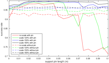
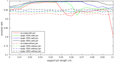
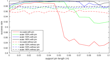
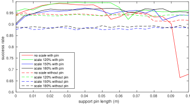
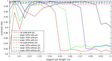
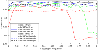
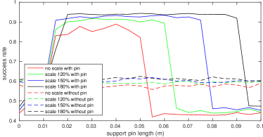
We further investigate the relationship between the size of an object and the success rate of the orientation task. Given an object, we resize it from the center on four different scales ($100\%$, $120\%$, $150\%$ and $180\%$), and repeat the above experiments for each scale. The results are shown in Figure 12. For each scale of the objects, the curves illustrating the relation between the pin length and the success rate is of the similar shape as the curves shown in Figure 11 for the unscaled objects. In addition, we find that when the object size increases, we can choose the pin length from a wider range but still achieve the optimal success rate.

((a)) $l$

((b)) $el$

((c)) $3t$

((d)) $3ts$

((e)) $3t2s$

((f)) $cross$

((g)) $t$

((h)) $1t1p$

Figure 12: Relations between the success rate and the object’s size while reorienting different models.

IV-F Relations between the Grasp Density and Success Rates

We also change the density of the total grasps by changing the number of sampled directions as mentioned in Section III-A3.

The results in Figure 13 illustrate the changing success rate with respect to various grasp density. In general the success rate of the orientation task improves as the number of sampled directions increases from $3$ to $8$, and the small fluctuation is due to the randomness in the experiment. We observe that the reorientation success rate increases when the grasp density increases. However, the performance improvement is small for grasp densities larger than $6$.

We also illustrate the grasp density’s influence on the timing cost of the regrasp graph construction and the regrasp grasp online search in Figure 14 and Figure 15, respectively. We can observe that the time cost while using the pin placement is generally slower than the time cost while using the planar placement, because the regrasp graph for the pin placement is more complicated. The $cross$ model is the only exception, where the regrasp graph of the pin placement has fewer connectivity due to the reason discussed in Section IV-C, and thus the timing cost of the pin placement is also lower.

According to these results, we conclude that a grasp density of $6$ can make a good tradeoff between the reorientation success rate and the time cost.

((a)) $l$

((b)) $el$

((c)) $3t$

((d)) $3ts$

((e)) $3t2s$

((f)) $cross$

((g)) $t$

((h)) $1t1p$

Figure 13: Relations between the success rate and the changing grasp density while reorienting the models.

((a)) $l$

((b)) $el$

((c)) $3t$

((d)) $3ts$

((e)) $3t2s$

((f)) $cross$

((g)) $t$

((h)) $1t1p$

Figure 14: Relations between the graph build time and the changing grasp density while reorienting the models.

((a)) $l$

((b)) $el$

((c)) $3t$

((d)) $3ts$

((e)) $3t2s$

((f)) $cross$

((g)) $t$

((h)) $1t1p$

Figure 15: Relations between the graph search time and the changing grasp density while reorienting the models.

IV-G Comparison of Regrasp Sequence Lengths

We also compare the number of regrasps used while using the pin placement to the number of regrasps used while using the planar placement. As shown in Figure 16, we can see that in general the two different placement settings will result in regrasp sequences with similar lengths. For the pot lid shape object $1t1p$, the sequence length while using the pin placement is significantly longer than the sequence length while using the planar placement. This is because the $1t1p$ is difficult to be oriented, and thus for the planar placement setting, many reorientation trials fail and are not counted in the computation of average length of regrasp sequences. While using the pin placement, the reorientation task has a higher success rate for difficult trials, but may require more regrasps to achieve the reorientation in such difficult cases.

Figure 16: Comparison between the average sequence length of the orientation task, while using two different placement settings. The red bars are the results using the added pin for placement, while the blue bars are the results only using the planar surface for support.

IV-H Spatial Distribution of Success Rates and Regrasp Sequence Lengths

Besides the average success rate and average regrasp sequence length computed over all trials as demonstrated in Section IV-C and Section IV-G, we also compute the average success rate and regrasp sequence length over the 10 trials for each grid in the working area. These data describe the spatial distribution of the success rate and sequence length for the reorientation task, and help us to have a better understanding about the difference between the different placement settings.

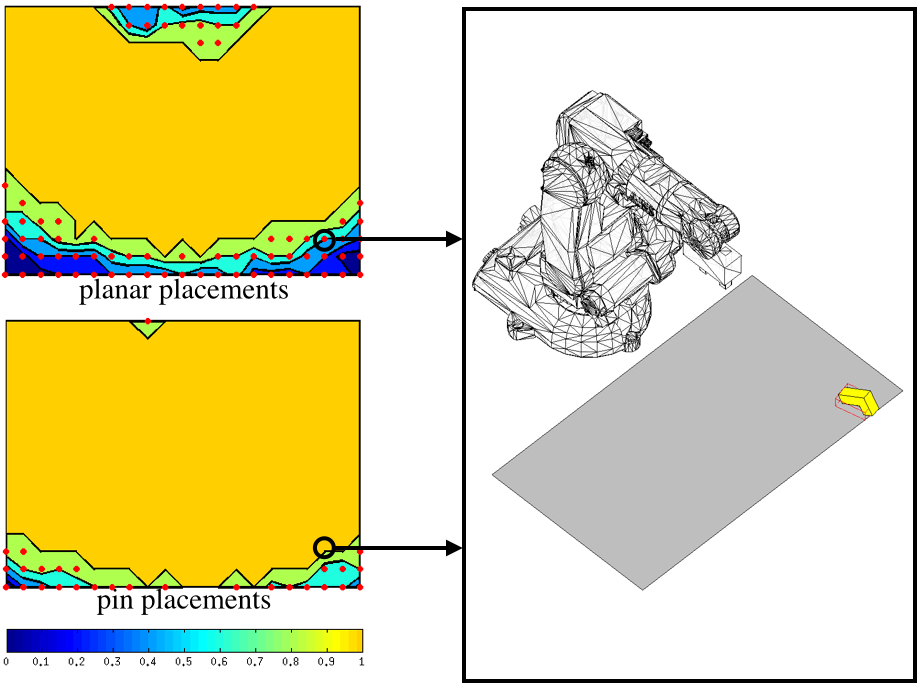
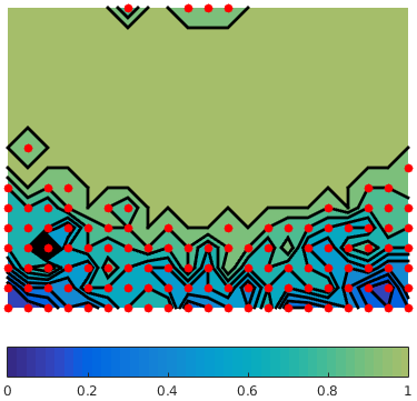
First, we compare the spatial distributions of the success rate while performing the reorientation task between two different placement settings for two objects $l$ and $1t1p$, and the results are shown in Figure 17 and Figure 18. In Figure 17, we also illustrate one trial where the reorientation task fails in the planar placement setting but succeeds in the pin placement setting. From the result for $l$ model in Figure 17, we can observe that, while using the pin placement, the robot will have a larger region in the workspace where the success rate is 100%. For other regions, the pin placement also provides a higher success rate than that of the planar placement. The contrast becomes more obvious for the pot lid like object $1t1p$ in Figure 18. We observe that the planar placement always has a non-zero failure possibility over the entire workspace, while the pin placement has a $100\%$ success rate over a large part of the workspace.

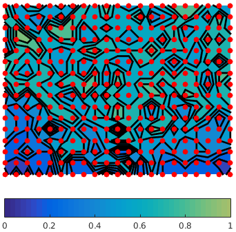
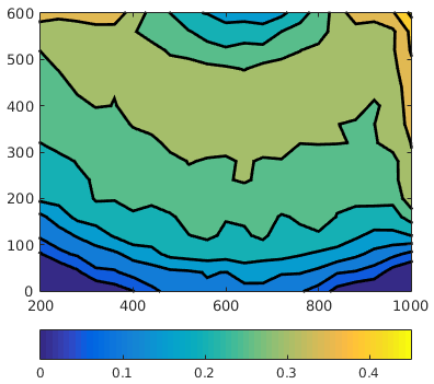
Note that the two placement settings’ difference in their spatial distributions of the success rate can be attributed mostly to the difference in the regrasp possibility between the two settings rather than the differences in the robotic arm’s kinematic reachability. To show this, in Figure 18(c) we demonstrate the robotic arm’s kinematic reachability, which is computed for a plane at the height of $h$ above the plane where the regrasp experiments are performed. Here, $h$ is the average height for the center of mass of all objects in different placements. The reachability is the same for different objects, but we can observe that the spatial distribution of the success rate is very different between $l$ and $1t1p$ using the planar placement. Such differences are mainly caused by the different regrasp possibilities of these two objects. Similarly, the reachability is roughly the same while using either the planar placement or the pin placement, but the spatial distribution over the success rate is greatly improved for the object $1t1p$ when using the pin placement instead of the planar placement. Such an improvement is mainly due to the improved regrasp possibility of the pin placement compared to that of the planar placement.

Figure 17: Comparison of the spatial distribution of the success rates between the pin placement and the planar placement while orienting the $l$ model. The robot is standing in the north side of the rectangle working space. The red points are the grid points where the reorientation task may fail, i.e., success rate is less than 100%. Different colors are used to visualize different values of success rate, ranging from 0 to 1. The right sub-figure shows one instance of the orientation task that fails while using the planar placement but succeeds while using the pin placement.

((a)) $1t1p$ planar placements

((b)) $1t1p$ pin placements

((c)) reachability

Figure 18: Comparison of the spatial distribution of the success rates between the pin placement and the planar placement while orienting the pot lid like object $1t1p$. The red points are the grid points where the reorientation task may fail, i.e., success rate is less than 100%. Different colors are used to visualize different values of success rate, ranging from 0 to 1. We also compute the reachability of the single arm, in order to demonstrate the difference between the spatial distribution of the success rates and the robotic arm’s reachability.

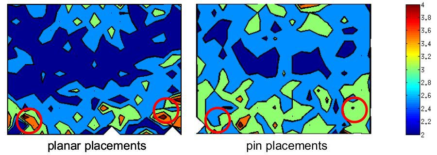
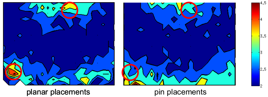
Next, we compare two different placement settings’ spatial distribution over the length of the regrasp sequence, as shown in Figure 19. We can observe in Figure 17 that for challenging regions where the success rate is relatively lower for both placements, the sequence length is shorter for the pin placement compared to the sequence length for the planar placement. This is because in these situations, reorientation is difficult and the pin placement’s highly connected regrasp graph is more likely to generate efficient regrasps. For other places in the center of the workspace where the success rate is closer to 100%, both placements have similar average lengths for regrasp sequences. The sequence using pin placements may be a bit longer sometimes, also because the placement set is larger for pin cases than for planar cases.

((a)) $1t1p$

((b)) $l$

Figure 19: Comparison of the spatial distribution of the regrasp sequence length between the pin placement and the planar placement while orienting $1t1p$ and $l$ models. The robot is standing in the north side of the rectangle working space. The regions marked by the red circles are challenging workspace where the success rate is relatively lower for both placements.

IV-I Assembly Tasks

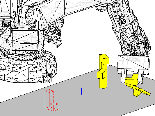
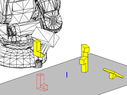
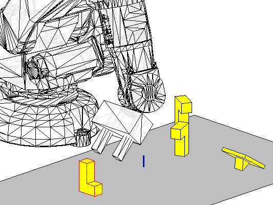
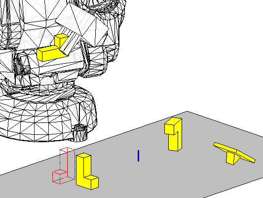
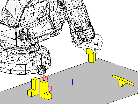
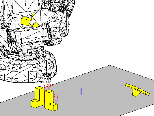
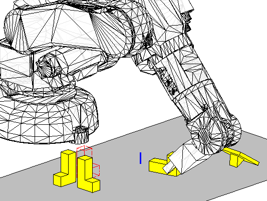
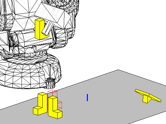
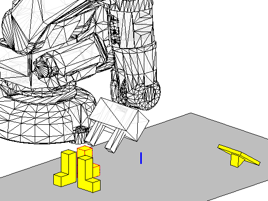
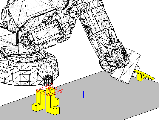
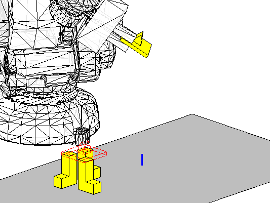
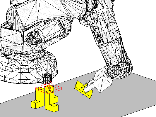
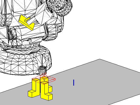
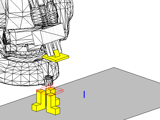
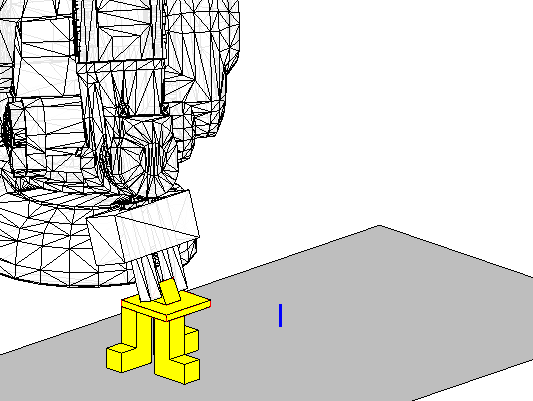
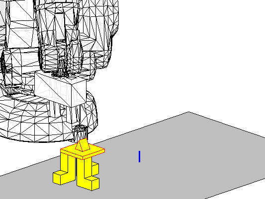
Moreover, we perform an assembly task in which the robot picks up components from one side of the working area and places them down at the other side to construct a predefined structure. During the process, the robot chooses suitable re-placement settings for transition on its own, i.e., the regrasp graph is a mixture of pin placements and planar placements. The resulting regrasp sequence is shown in Figure 20. We can see that the first object can be directly reoriented without regrasp, while the next two objects achieve the regrasp only using the planar support. The final pot lid like object is the most challenging one. The task of placing it on top of the other components is impossible without using the pin for an intermediate placement. This task is also achievable by only using the pin placement setting, but is not possible while only using the planar placement setting. This proves the efficacy of a support pin placement in challenging assembly tasks.

((a))

((b))

((c))

((d))

((e))

((f))

((g))

((h))

((i))

((j))

((k))

((l))

((m))

((n))

((o))

((p))

((q))

((r))

((s))

((t))

((u))

((v))

((w))

((x))

Figure 20: The regrasp sequence for assembling four different objects, including one pot lid like object. The sequence is computed with the two-layer regrasp graph built on the grasps computed by sampling the mesh models. The first object is oriented without regrasp (b)-(d). All other objects require one step of regrasp: the second and the third object use the planar placement for regrasping, and the transition steps occurs at (g)-(h) and (m)-(n), respectively. The final object is of the pot lid shape, and the robot must leverage the pin placement to successfully reorient the object, and the transition happens at (s)-(t).

V Conclusion

In this paper, we improve the pick-and-place regrasp planning by using an added support pin for intermediate placements. We demonstrate that by using the pin placements, we can improve the connectivity of the regrasp graph, and eventually increase the success rate of the reorientation task for objects with various shapes. We perform a large number of experiments to empirically investigate how the performance of the reorientation task is influenced by a variety of factors, including the pin length, the object’s size, the object’s shape, and the grasp density. Moreover, we also show one challenging assembly task which is not possible without the pin placements.

There are many directions for future work. First, we would like to learn a closed form expression for the relation between the reorientation success rate, the pin length, and the object size, by collecting a large amount of training data from repeated experiments. The learned formulation can be used to compute the optimal pin length for a given reorientation task. Second, our current regrasp planning framework does not take into the uncertainty that is ubiquitous in the real-world applications. For instance, our method assumes the validity of the placements and grasps to be solely determined by the geometric shape of the object, which is not true in reality since the (unknown) physical properties of the object (e.g., whether the object is made of wood, plastic, or light metal like aluminum) are also important for the grasp quality. We plan to design some robustness criteria for the placements and grasps (e.g., the torque constraints) in order to filter out all unstable grasps and achieve a robust regrasp sequence. Eventually, we are interested in implementing the entire framework on real industrial robots for challenging manufacturing tasks such as 3C assembly.

References

- [1] P. Tournassoud, T. Lozano-Perez, and E. Mazer, “Regrasping,” in IEEE International Conference on Robotics and Automation, vol. 4, 1987, pp. 1924–1928.
- [2] W. Wan, M. Mason, R. Fukui, and Y. Kuniyoshi, “Improving regrasp algorithms to analyze the utility of work surfaces in a workcell,” in IEEE International Conference on Robotics and Automation, 2015, pp. 4326–4333.
- [3] T. Lozano-Pérez, J. L. Jones, P. A. O’Donnell, and E. Mazer, Handey: A Robot Task Planner. Cambridge, MA, USA: MIT Press, 1992.
- [4] H. Terasaki and T. Hasegawa, “Motion planning of intelligent manipulation by a parallel two-fingered gripper equipped with a simple rotating mechanism,” IEEE Transactions on Robotics and Automation, vol. 14, no. 2, pp. 207–219, Apr 1998.
- [5] W. Wan, E. Cheung, J. Pan, and K. Harada, “Optimizing the parameters of tilting surfaces in robotic workcells,” in IEEE International Conference on Automation Science and Engineering, 2015.
- [6] K. Harada, T. Tsuji, K. Nagata, N. Yamanobe, and H. Onda, “Validating an object placement planner for robotic pick-and-place tasks,” Robotics and Autonomous Systems, vol. 62, no. 10, pp. 1463–1477, Oct. 2014.
- [7] M. Schuster, J. Okerman, H. Nguyen, J. Rehg, and C. Kemp, “Perceiving clutter and surfaces for object placement in indoor environments,” in IEEE-RAS International Conference on Humanoid Robots, 2010, pp. 152–159.
- [8] T. Lozano-Perez and L. Kaelbling, “A constraint-based method for solving sequential manipulation planning problems,” in IEEE/RSJ International Conference on Intelligent Robots and Systems, 2014, pp. 3684–3691.
- [9] Y. Jiang, M. Lim, C. Zheng, and A. Saxena, “Learning to place new objects in a scene,” International Journal of Robotics Research, vol. 31, no. 9, pp. 1021–1043, Aug. 2012.
- [10] J. Baumgartl, T. Werner, P. Kaminsky, and D. Henrich, “A fast, gpu-based geometrical placement planner for unknown sensor-modelled objects and placement areas,” in IEEE International Conference on Robotics and Automation, 2014, pp. 1552–1559.
- [11] H. Fu, D. Cohen-Or, G. Dror, and A. Sheffer, “Upright orientation of man-made objects,” ACM Transactions on Graphics, vol. 27, no. 3, pp. 42:1–42:7, 2008.
- [12] D. J. Kriegman, “Let them fall where they may: Capture regions of curved objects and polyhedra,” International Journal of Robotics Research, vol. 16, no. 4, pp. 448–472, 1997.
- [13] M. Moll and M. A. Erdmann, “Manipulation of pose distributions,” International Journal of Robotics Research, vol. 21, no. 3, pp. 277–292, 2002.
- [14] T. Siméon, J.-P. Laumond, J. Cortés, and A. Sahbani, “Manipulation planning with probabilistic roadmaps,” The International Journal of Robotics Research, vol. 23, no. 7-8, pp. 729–746, 2004.
- [15] K. Hauser and V. Ng-Thow-Hing, “Randomized multi-modal motion planning for a humanoid robot manipulation task,” The International Journal of Robotics Research, vol. 30, no. 6, pp. 678–698, 2011.
- [16] F. Lagriffoul, D. Dimitrov, A. Saffiotti, and L. Karlsson, “Constraint propagation on interval bounds for dealing with geometric backtracking,” in IEEE/RSJ International Conference on Intelligent Robots and Systems, 2012, pp. 957–964.
- [17] M. Dogar, A. Spielberg, S. Baker, and D. Rus, “Multi-robot grasp planning for sequential assembly operations,” in IEEE International Conference on Robotics and Automation, 2015, pp. 193–200.
- [18] B. Carlisle, K. Goldberg, A. Rao, and J. Wiegley, “A pivoting gripper for feeding industrial parts,” in IEEE International Conference on Robotics and Automation, 1994, pp. 1650–1655.
- [19] E. Yoshida, M. Poirier, J.-P. Laumond, O. Kanoun, F. Lamiraux, R. Alami, and K. Yokoi, “Pivoting based manipulation by a humanoid robot,” Auton. Robots, vol. 28, no. 1, pp. 77–88, Jan. 2010.
- [20] K. Lynch and M. Mason, “Stable pushing: Mechanics, controllability, and planning,” International Journal of Robotics Research, 1996.
- [21] N. Chavan-Dafle and A. Rodriguez, “Prehensile pushing: In-hand manipulation with push-primitives,” in IEEE/RSJ International Conference on Intelligent Robots and Systems, 2015.
- [22] N. Chavan-Dafle, A. Rodriguez, R. Paolini, B. Tang, S. S. Srinivasa, M. Erdmann, M. T. Mason, I. Lundberg, H. Staab, and T. Fuhlbrigge, “Extrinsic dexterity: In-hand manipulation with external forces,” in IEEE International Conference on Robotics and Automation, 2014.
- [23] G. Lee, T. Lozano-Perez, and L. P. Kaelbling, “Hierarchical planning for multi-contact non-prehensile manipulation,” in IEEE/RAS International Conference on Intelligent Robots and Sytems, 2015.
- [24] S. Jentzsch, A. Gaschler, O. Khatib, and A. Knoll, “MOPL: A multi-modal path planner for generic manipulation tasks,” in IEEE/RSJ International Conference on Intelligent Robots and Systems, 2015.
- [25] Y. Koga and J.-C. Latombe, “On multi-arm manipulation planning,” in IEEE International Conference on Robotics and Automation, 1994, pp. 945–952.
- [26] N. Vahrenkamp, D. Berenson, T. Asfour, J. Kuffner, and R. Dillmann, “Humanoid motion planning for dual-arm manipulation and re-grasping tasks,” in IEEE/RSJ International Conference on Intelligent Robots and Systems, 2009, pp. 2464–2470.
- [27] B. Cohen, S. Chitta, and M. Likhachev, “Search-based planning for dual-arm manipulation with upright orientation constraints,” in IEEE International Conference on Robotics and Automation, 2012, pp. 3784–3790.
- [28] A. Dobson and K. E. Bekris, “Planning representations and algorithms for prehensile multi-arm manipulation,” in IEEE/RAS International Conference on Intelligent Robots and Sytems, 2015.
- [29] B. Cohen, M. Phillips, and M. Likhachev, “Planning single-arm manipulations with n-arm robots,” in Robotics: Science and System, 2015.