The topological effect on the Mechanical properties of polymer knots

Abstract

The mechanical properties of polymer knots under stretching in a bad or good solvent are investigated by applying a given force $F$ to a point of the knot while keeping another point fixed. The Monte Carlo sampling of the polymer conformations on a simple cubic lattice is performed using a variant of the Wang-Landau algorithm. The results of the calculations of the specific energy, specific heat capacity and gyration radius for several knot topologies show a general trend in the behavior of short polymer knots with lengths up to seventy lattice units. At low tensile force $F$, knots can be found either in a compact or an extended phase, depending if the temperature is low or high. At any temperature, with increasing values of the force $F$, a polymer knot undergoes a phase transition to a stretched state. This transition is characterized by a strong peak in the heat capacity. There is also a minor peak, which corresponds to a transition occurring at low temperatures when the conformations of polymers in the stretched phase become swollen with increasing temperatures. It is also shown that the behavior of short polymer rings is strongly influenced by topological effects. The limitations in the number of accessible energy states due to topological constraints is particularly evident in knots of small size and such that their minimum number of crossing according to the Rolfsen knot table is high. An example is provided by a cinquefoil knot $5_{1}$ with a length of only fifty lattice units. The thermal and mechanical properties of knots that can be represented with diagrams having the same minimum number of crossings, are very similar. The size effects on the behavior of polymer knots have been analyzed too. Surprisingly, it is found that topological effects fade out very fast with increasing polymer length.

I Introduction

Closed polymer rings with nontrivial topological properties are a major pattern in nature. The formation of DNA knots is a phenomenon that has been observed in all the three domains of life d1 ; d2 . Bacterial DNA often occurs in the form of knots that are sometimes heavily linked together. Knots are present also in the DNA of viruses. For instance, it has been shown that 95% of the DNA molecules extracted from tailless mutants of phage P4 vir 1 del22 are highly knotted per95 . Knots appear in proteins too, although not so frequently as in DNA d3 . So far, the following knots have been found in proteins: the trefoil knot $3_{1}$, the figure-eight knot $4_{1}$, the penta knot $5_{2}$ and the Stevedore knot $6_{1}$ 61knot . It should be however recalled that the trajectories of proteins are open, so that their knots do not sustain the full topological properties of mathematical knots.

The synthesis of artificial polymer knots and links has been realized more than twenty years ago and there have been in this subject many new developments Dietrich-Buchecker1989 ; schappacher ; ohta2009 ; Ohta2012 . For example, the first artificial trefoil knot has been synthesized by Dietrich-Buchecker et al. Dietrich-Buchecker1989 in 1989, while knotted ring polystyrene with high molecular weight has been successfully synthesized by intramolecular cyclization reactions in poor solvents by Ohta et al. Ohta2012 . The presence of knots has several consequences on the behavior of polymer materials which, most important, are measurable in experiments and may be used to test theoretical results, see for example Arai1999 ; Saitta1999 ; levene ; trigueiros ; s2 ; s3 ; elbaz ; radloff ; likos ; electrophoresis2 ; nahum ; k2008 ; Hossain . Very recently, the paper newpaper appeared with an updated list of advances and references. Topological effects in the glass transition of polymer knots have been tested using the methods of calorimetry in HossainPhD .

Analytically, more specifically using the methods of field theory and renormalization group theory that have been so successful in the case of linear polymer chains, up to now it is possible to study only linked polymers rings, the so-called catenanes FFIL2 ; FFAP ; FFIL ; FFIL3 . Despite several efforts, we cite here only the most recent ones ffmpyz ; rohwer , there is still no analytical model for polymer knots. For this reason, in this work the properties of a single knot subjected to a tensile force will be investigated numerically. For our purposes, it will be convenient to use the particular variant newwl of the original Wang-Landau Monte Carlo algorithm wl . Both the original algorithm and the variant have been already applied to polymer physics Velyaminov ; swetnam ; yzff ; yzff2013 . We choose the strategy of starting from a given seed conformation of the knot to be investigated. The original seed conformation is later changed using a set of random transformations called the pivot moves pivot . Random transformations are used both for the equilibration of the seed and for sampling a statistically relevant set of knot conformations. The topology after each transformation is preserved with the help of the PAEA method, first introduced in yzff . Our studies are performed on a simple cubic lattice and in the so-called stress ensemble, in which the tensile forces and their application points are regarded as the known ”thermodynamical” parameters. The variables conjugated to the forces are the average distances at equilibrium of the application points with respect to a set of reference points, lines or planes. These distances are evaluated numerically. The Hamiltonian is that already used in Refs. yzff ; yzff2013 with the addition of a mechanical term describing a constant force $F$ pulling the knot at one point while another point is anchored at one site of the lattice.

The goal pursued in this work is to understand how a polymer knot behaves under stretching at different temperatures. So far, there have been few studies of this kind. When no external forces are applied, an exhaustive investigation of the thermal properties of linear open chains can be found in binder . For very short-range interactions, as those considered in that work, it turns out that the heat capacity of linear open chains in a bad solvent, plotted as a function of the temperature, exhibits a single sharp peak corresponding to a phase transition from a crystallite state to an expanded coil state. Such phase transitions occur at low temperatures and are usually related to states which are very compact and thus statistically rare. The thermal properties of unstretched polymer knots on a single cubic lattice have been the subject of Refs. yzff ; yzffappleb ; yzff2013 . Also in the case of knots, a close inspection of the conformations shows that, in a bad solvent, ordered compact structures are forming at low temperatures, corresponding to the crystallite phase. At higher temperatures, the knot is found in an expanded state. The heat capacity is characterized by a single peak, corresponding to the phase transition from the crystallite to the expanded state. The behavior of the specific energy of the knot and its gyration radius confirms this conclusion. The crystallite–expanded state transition does not seem to be a lattice artifact or a pseudo-phase transition as those discussed in Ref. vogel . Indeed, the height of the peak grows proportionally to the number of segments $N$ composing the knot at least up to the maximum length we could check so far ($N=2100$). Similar results were also found in the work Velyaminov , where the statistical properties of unknotted rings, the so-called unknots, have been studied. Up to now it is still unclear if there are other phase transitions occurring starting from phases in which the polymer knot finds itself in a particular set of conformations that are extremely rare. The existing studies of very short polymer rings with no knotting confirm the presence of a single peak in the heat capacity Velyaminov ; yzff . The case of knotted rings is complicated by the difficulties of sampling extremely compact conformations, which will be discussed in more details in Subsection II.3.

The phase diagram of polymer knots becomes more interesting when tensile forces are applied. The heat capacity and other observables can then be plotted as a function of both the temperature $T$ and the force $F$. As already shown in swetnam , in this extended two-dimensional space of parameters new phases appear. In Ref. swetnam , however, a different setup has been used, in which the variable conjugate to the force $F$ is the height of the knot along the $z-$axis. This setup is related to the compression and elongation of a knot rather than to stretching. The two approaches are not equivalent. In our case the expectation values of observables like the specific energy, the specific heat capacity and the gyration radius are symmetric under the change of the orientation of the force $F$. This is not true within the approach of swetnam , because by inverting the sign of $F$ one passes from compression to extension, which clearly are not equivalent processes. Of course, the properties of the knot under stretching should be similar to those found in swetnam when the polymer is elongated. Indeed, we have verified that this is the case. As a consistency check, we have also reproduced part of the results of swetnam using their setup.

It turns out from our computations that the phase diagram of short polymer knots is quite diversified and that the topology of the knot has a strong impact on its behavior. For small stretching forces, the system undergoes only one phase transition from a crystallite state to an expanded state. This transition occurs when the temperature increases and it was already found in yzff . Additionally, there is another phase transition which takes place at any given temperature when the knot is pulled by a tensile force. This transition consists in the passage from an unstretched phase (crystallite or expanded depending if the temperature is low or high) to a stretched phase. At low temperatures and for high stretching forces, there is an additional transition from a stretched but more compact phase to a stretched and more expanded phase.

We have analyzed also the possible effects of topology and size on the mechanical and thermal properties of polymer knots. The case of the thermal properties of unstretched polymers has already pointed out that topology plays an important role when polymer is short and the monomers are strongly interacting, see e. g. Ref. yzff2013 . In that reference it was also established that the behavior of a knotted polymer ring starts to be independent of the knot type when its length exceeds approximately that of $400$ lattice units yzff2013 . The knots considered in this paper are much shorter than that and, indeed, we have found that there are effects related to topology which are relevant and visible in the plots of the computed observables. Strong topological effects on the mechanical properties of knots are related to the fact that, in more complex knots, the polymer trajectories need to perform more turns in order to obey the topological constraints. For this reason, the number of possible conformations is limited and it is much harder to stretch complex knots than simpler ones. Knots that can be constructed with the same minimal number of crossings like $5_{1}$ and $5_{2}$ do not show many differences in their behavior. We find also that the strength of the topological effects fades out very rapidly when the polymer length is growing. These facts can be seen from the plots of the specific energy, specific heat capacity and gyration radius, whose expectation values have been computed in the present work.

The presented material is organized as follows. The setup of the simulations performed, including the Wang-Landau sampling strategy and the formulas used to compute the observables, will be explained in Section II. The set of observables consists in the specific energy, specific heat capacity and gyration radius. The results concerning the mechanical properties are presented in Section III. In order to detect possible effects of topology on the behavior of polymers, several types of knots of different lengths have been considered: the unknot $0_{1}$, the trefoil knot $3_{1}$, the knots $5_{1}$, $5_{2}$ and $7_{1}$. The size effects have been investigated focusing on polymer rings of different lengths but with the same topology, namely that of the trefoil knot $3_{1}$. Finally, in Section IV our conclusions are drawn and possible generalizations of this work are discussed.

II Methodology

II.1 Polymer model on a simple cubic lattice

In this work, the mechanical properties of polymer knots under stretching are studied on a simple cubic lattice. The Hamiltonian $H_{X}$ of a polymer knot composed by $N$ segments can be written as follows:

$$H(X)=m\varepsilon-Fd_{z}$$ (1)

The symbol $X$ represents a suitable set of variables needed to describe the conformation of the knot in space. The first term in the right hand side of Eq. (1) describes very short-range interactions between pairs of non-bonded monomers. $m$ is the number of contacts, i. e. the number of pairs of non-bonded monomers in a given conformation $X$ whose reciprocal distance amounts to one lattice unit. $\varepsilon$ is the energy cost for one contact. If $\varepsilon>0$ the interactions are repulsive and correspond to the situation in which the polymer is in a good solvent. If $\varepsilon<0$, instead, the attractive interactions typical of bad solvents are obtained.

The second term of Eq. (1) is the potential associated to a constant force $F$ directed along the $z-$axis and applied to the point $\boldsymbol{R}_{\frac{N}{2}+1}$ of the knot. Here $\boldsymbol{R}_{1},\ldots,\boldsymbol{R}_{N}$ denote the locations of the $N$ monomers composing the knot. The first monomer $\boldsymbol{R}_{1}$ is fixed in the origin. $d_{z}$ is the $z-$component of the vector $\boldsymbol{R}_{\frac{N}{2}+1}-\boldsymbol{R}_{1}$, See Fig. 1 for a pictorial representation of our set-up.

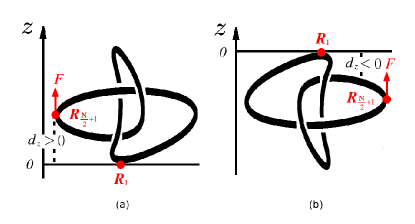
Figure 1: The known force $F$ is applied to the point $\boldsymbol{R}_{\frac{N}{2}+1}$ of a trefoil knot. The orientation of the force $F$ is along the direction of positive $z$. (a) The value of $d_{z}$ is positive, i. e. $d_{z}>0$; (b) The value of $d_{z}$ is negative, i. e. $d_{z}<0$.

To check the consistency of our code, we repeat the calculations of the specific heat capacity for an unknot presented in swetnam . In that work, the thermodynamic parameters are the force $F$ directed along the $z-$axis and the height $h_{X}$ in the $z$ direction of the conformation $X$, see Fig. 2.

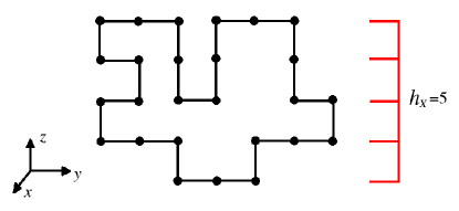
Figure 2: The height $h_{X}$ of the conformation $X$ along the $z$ axis.

Clearly, $h_{X}>0$ while $F$ can take both positive and negative values, corresponding to stretching and compression respectively. With this setting, the phase diagram of lattice polymer rings under stretching has been determined in Ref. swetnam in the case of a few knots subjected to attractive interactions ($\varepsilon<0$). Our results are quantitatively coinciding with the calculation of swetnam . For example, the specific heat capacity of an unknot with 36 segments displayed in Fig. 3 is in agreement with the corresponding result appearing in Fig. 16 of Ref. swetnam .

Figure 3: Plot of the specific heat capacity of an unknot $0_{1}$ with 36 segments with respect to the force $F$. The force is directed along the $z−$axis. Its orientation depends on the sign of $F$.

II.2 Sampling strategy

The sampling strategy pursued in this work consists in starting from a given seed conformation and then changing it with random transformations in order to obtain a statistically relevant set of conformations. The sampling itself is performed applying the variant of the Wang-Landau Monte Carlo algorithm of Ref. newwl and that will be discussed below. Before applying the Monte Carlo algorithm, the initial seed conformation is subjected to random changes in order to equilibrate it. The equilibrating procedure and the criteria for deciding when equilibrium is reached have been illustrated in yzff . The random transformations used in this work both for equilibration and sampling are the so-called pivot moves pivot . Although a formal proof of the ergodicity of these transformations in the case of knots does not yet exist, our previous simulations provide enough evidence about it yzff ; yzff2013 . It is possible to construct pivot moves that are able to change an arbitrary number of contiguous segment $k<N$ of a polymer knot. When the polymer conformations are swollen, higher values of $k$ are better, because a larger part of the knot is changed and in this way the convergence of the Wang-Landau algorithm is sped up. For very compact conformations, instead, small values of $k$ are preferable, because the likelihood that a pivot move breaks the topology of the knot grows with $k$ and becomes very high when monomers are densely packed together. If too many pivot moves must be rejected to avoid that the topology is modified, the time necessary to finish successfully a simulation may increase considerably. It has been found in yzff2013 that a convenient approach consists to choose pivot moves in which $k$ may vary randomly within a given interval of values.

In general, pivot moves with $k>3$ are potentially violating the topology of knot. In order to preserve it, it will be used here the PAEA (Pivot Algorithm and Excluded Area) method, which has been developed in yzff . As shown in yzff , the time required within this method to avoid topology changes during the sampling procedure is proportional to the number of segments of a given polymer. This feature makes the PAEA method one of the fastest method on the market.

The goal of the sampling strategy explained above is to determine the density of states of a polymer knot. The density of states is the crucial ingredient in the calculation of the averages of any macroscopic observable in the microcanonical ensemble.

II.3 The sampling algorithm

The Wang-Landau method consists in a step-by-step procedure that allows to derive within the microcanonical ensemble the density of states $\phi_{E}$ in a given interval of the energy $E$. At each step, the accuracy of the computation of $\phi_{E}$ depends on a parameter called the modification factor wl , which must decrease in a suitable way in order to increase the degree of the accuracy. In the original version of the method, the modification factor starts from the initial value $f_{0}=e$ and is reduced at each further step $\nu=1,2,\ldots,\nu_{max}$ according to the rule $f_{\nu}=\sqrt{f_{\nu-1}}$ wl .

A few variants aiming to improve the Wang-Landau algorithm first established in wl have been recently proposed. For instance, in 1twl it has been shown that the way in which the modification factor is reduced affects the convergence of the algorithm to the exact value of $\phi_{E}$. An improved prescription for decreasing the modification factor, called the $1/t$ Wang-Landau method, has been presented in 1twl . For our purposes, suitable algorithms are those which take into account the fact that polymer knots are systems characterized by a rough energy landscape and have an energy range that is a priori unknown. The reason for which the energy range is undetermined is that, even for a simple Hamiltonian like that of Eq. (1), the analytical calculation of the maximum number of contacts $m$ of a knot on a cubic lattice is difficult. When attempting to find numerically the highest value of $m$, which in the case of attractive interactions and fixed force $F$ corresponds to the absolute minimum of the Hamiltonian (1), one encounters several, if not many relative minima, from which it is not easy to escape using random transformations. As a consequence, occasionally the system gets trapped at some point of relative minimum. All that seems to suggests that a polymer knot could have a rough energy landscape with a complex structure. The complexity of the energy landscape is related to the problem of sampling extremely rare conformations mentioned in the Introduction. Indeed, conformations with very high contact number, corresponding to energy minima when the interactions are attractive, have to be considered as events that are very rare and thus hard to be sampled yzff2013 . The existence of such events slows down the calculation of the density of states considerably. For instance, even in the case of a short polymer with $N=70$ segments, a conformation with $m=84$ contacts is normally discovered after generating tens of billions of conformations. In this situation, it is easy to realize that, without a careful treatment of rare events, a rare conformations may appear for the first time when the simulation is already in an advanced stage, i. e. when it is very likely that the modification factor will be small due to the reduction procedure briefly discussed before. If this happens, the algorithm is trapped into the rare configuration until the density of state $\phi_{E}$ for the corrisponding energy value is computed. This calculation must be performed with a high accuracy because the modification is small and thus requires a very long time. A simple solution to this problem is to set a cutoff in the maximum value of $m$ yzff2013 ; binder . In this way, the sampling of extremely compact or swollen conformations is prevented. The disadvantage of this procedure is that the exclusion of conformations with a higher number of contacts may result in a poor description of the thermal properties of the polymer at low temperatures if the interactions are attractive binder . Moreover, with an inappropriate choice of the energy cutoffs, those phase transitions that are taking place at low temperatures and thus involve very compact conformations, see for example binder ; wl2 , may be neglected.

Motivated by the need of dealing with the above difficulties, in the present work the conformations of polymer knots will be sampled with the help of the variant of the Wang-Landau method explained in Ref. newwl . This variant has been explicitly developed in order to cope with systems with a rough energy landscape and a energy range which is not fixed as it is in the present situation.

Finally, let us note that, according to the Hamiltonian of Eq. (1), the energy of a conformation $X$ depends on the force $F$, the number of contacts $m$ and the distance $d_{z}$. In the following, it will be convenient to compute the density of state as a function of $m$ and $d_{z}$. Thus, the density of state will be denoted hereafter with the symbol $\phi_{m,d_{z}}$. During the sampling procedure, the transition probability from a microstate $X_{m,d_{z}}$ to another microstate $X_{m^{\prime},d_{z}^{\prime}}$ will be given by:

$$P(X_{m,d_{z}}\longrightarrow X_{m^{\prime},d_{z}^{\prime}})=\min\left[1,\frac{\phi_{m,d_{z}}}{\phi_{m^{\prime},d_{z}^{\prime}}}\right]$$ (2)

The modification factor $F_{new}$ is choosen using the prescriptions of Refs. newwl ; wl2 adapted to the present case:

$$F_{new}=p\sum_{i=1}^{N_{m}}\sum_{j=1}^{N_{d}}\left(\frac{M(m_{i},d_{z,i})}{\sum_{i=1}^{N_{m,d}}\sum_{j=1}^{N_{d}}M(m_{i},d_{z,j})}\right)^{2}-\frac{p}{N_{m}N_{d}}$$ (3)

In the above equation we have supposed that the possible values of the number of contacts $m$ and of the distance $d_{z}$ are labeled by indices $i=1,\ldots,N_{m}$ and $j=1,\ldots,N_{d}$ respectively. Of course, for a knot with $N$ segments, $N$ being an even integer, we have that $-\frac{N}{2}<d_{z,j}<+\frac{N}{2}$. Moreover $m_{i}=0,1,\ldots,m_{max}$. For a trefoil knot with $N=70$ the maximum number of contacts found after generating one hundred of billions of random conformations is $85$. For a general knot of arbitrary length, both the upper limit $m_{max}$ of the number of contacts and the boundaries of the interval of the allowed values of $d_{z}$ are difficult to be determined. For this reason, the boundary limits of both $m$ and $d_{z}$ are kept open during the whole simulation. This means that the integers $N_{m}$ and $N_{d}$ can change whenever it is accepted a new conformation, in which the number of contact, the distance $d_{z}$ or both have not been detected in the previously sampled conformations. For example, $N_{m}\longrightarrow N_{m}+1$ if the new conformation is characterized by a value of $m$ that was not encountered before. $M(m_{i},d_{z,j})$ is the energy histogram. It depends on $m$ and $d_{z}$ for convenience, but the energy $H(X_{i})$ of the conformation $X_{i}$ can be easily derived once the values of $m$ and $d_{z}$ are known: $H(X_{i})=m_{i}\varepsilon-Fd_{z,i}$. The initial value of $M(m_{i},d_{z,j})$, before the first conformation with $m=m_{i}$ and $d_{z}=d_{z,j}$ is discovered, is set to zero. When at some step of the simulation a conformation $X$ is accepted with number of contacts $m=m_{i}$ and distance $d_{z}=d_{z,j}$, then $M(m_{i},d_{z,j})$ is updated as follows: $M(m_{i},d_{z,j})\rightarrow M(m_{i},d_{z,j})+1$. Simultaneously, the value of the modification factor $F_{new}$ is set using Eq. (3). The prefactor $p$ appearing in that equation is a tuneable parameter. Its value depends on the system under investigation. In our simulations, $p$ has been set to be equal to one. The prescription for reducing the modification factor $F_{new}$ given in Eq. (3) has been obtained in wl2 by requiring that the convergence of the Wang-Landau algorithm to the density of state, estimated using a suitable function of the probability distribution of the data during the sampling, is optimized. This variant of the Wang-Landau algorithm has been proved to be particularly effective in the case of short polymer knots and with densities of states depending on more than one variable swetnam . It is easy to show that Eq. (3) can be cast also in the form:

$$F_{new}=p\sum_{i=1}^{N_{m}}\sum_{j=1}^{N_{d}}\left(\frac{M(m_{i},d_{z,j})}{\sum_{i=1}^{N_{m}}\sum_{j=1}^{N_{d}}M(m_{i},d_{z,j})}-\frac{1}{N_{m}N_{d}}\right)^{2}$$ (4)

so that $F_{new}\geq 0$ as it should be. In the optimized Wand-Landau algorithm of newwl , the transition probability $p(i\rightarrow i^{\prime})$ is the same of that of the original method, i. e. in our case is given by Eq. (2). The difference is that the modification factor $F_{new}$ shown in Eq. (3) needs to be updated after each Monte Carlo move, because it depends on the values of the energy histogram. Moreover, if the visited state is a new one, which has never been explored before, the values of $N_{m}$ and $N_{d}$, which are used to count the number of all distinct energy states, can change as mentioned before. The sampling procedure is continued until a flat energy histogram of all distinct energy states is reached. The flatness of the histogram is assessed within a $20\%$ of accuracy. It is easy to check that, if the histogram is ideally flat, $F_{new}$ vanishes identically.

II.4 Observables

By assuming thermodynamic units in which the Boltzmann constant is set to be equal to one, the partition function of the studied system may be written as follows:

$$Z(T,F)=\sum_{m}\sum_{d_{z}}\phi_{m,d_{z}}e^{-(m\varepsilon-Fd_{z})/T}$$ (5)

For any given value of the temperature $T$ and the force $F$, the density of states $\phi_{m,d_{z}}$ is derived by sampling over all microstates $X_{m,d_{z}}$ with fixed number $m$ of contacts and fixed $d_{z}$ swetnam . By using the knowledge of $\phi_{m,d_{z}}$, the average value of any observable ${\cal O}(m,d_{z})$ depending on $m$ and $d_{z}$ can be easily defined:

$$\langle{\cal O}(m,d_{z})\rangle(T,F)=\frac{\sum_{m}\sum_{d_{z}}{\cal O}(m,d_{z})\phi_{m,d_{z}}e^{-(m\varepsilon-Fd_{z})/T}}{Z(T,F)}$$ (6)

For example, the specific energy and the specific heat capacity are respectively given by:

$$\frac{\langle E\rangle(T,F)}{N}=\frac{1}{N}\dfrac{\sum_{m}\sum_{d_{z}}(m\varepsilon-Fd_{z})\phi_{m,d_{z}}e^{-(m\varepsilon-Fd_{z})/T}}{Z(T,F)}$$ (7)

$$\frac{C(T,F)}{N} = \frac{1}{N}\left[\frac{\langle m^{2}\rangle-\langle m\rangle^{2}}{T^{2}}\varepsilon^{2}+F^{2}\left(\frac{\langle d_{z}^{2}\rangle-\langle d_{z}\rangle^{2}}{T^{2}}\right)\varepsilon^{2}\right.$$ (8)

$$\left.-2F\left(\frac{\langle md_{z}\rangle-\langle m\rangle\langle d_{z}\rangle}{T^{2}}\right)\varepsilon\right]$$

where $\langle\ldots\rangle$ denotes the operation of averaging with respect of all possible conformations $X_{m,d_{z}}$ at given $T$ and $F$. The mean square radius of gyration $\langle R_{G}^{2}\rangle(T,F)$ will be computed according to the formulas:

$$\langle R_{G}^{2}\rangle(T,F)=\dfrac{\sum_{m}\sum_{d_{z}}{\langle R_{G}^{2}\rangle_{m,d_{z}}}\phi_{m,d_{z}}e^{-(m\varepsilon-Fd_{z})/T}}{Z(T,F)}$$ (9)

where $R_{G}^{2}=\frac{1}{2N^{2}}\sum_{I,J=1}^{N}(\boldsymbol{R}_{I}-\boldsymbol{R}_{J})^{2}$ and $\langle R_{G}^{2}\rangle_{m,d_{z}}$ is the average of $R_{G}^{2}$ restricted to states $X_{m,d_{z}}$ with $m$ contacts and distance $d_{z}$.

III Results

The topological and size effects on the mechanical and thermal behavior of polymer knots under stretching are the main subject of this Section. To check the topological effects we have considered different types of knots with the same number of segments $N$. The size effects have been investigated instead by fixing the knot type and changing its length. As already mentioned, throughout this paper thermodynamic units are used in which $k_{B}=1$, where $k_{B}$ is the Boltzmann constant. Moreover, the energy is counted in units of $\varepsilon$, so that it will be convenient to introduce the dimensionless energy unit $\mathbf{T}$ defined as follows:

$$\mathbf{T}=\frac{T}{|\varepsilon|}$$ (10)

Also the force $F$ will be normalized introducing the rescaled quantity:

$$\mathbf{F}=\frac{F}{|\varepsilon|}$$ (11)

$\mathbf{F}$ has the dimension of the inverse of a length. After this rescaling of variables, it is possible to define the normalized Hamiltonian ${E}(X)$ such that:

$$H(X)=|\varepsilon|E(X)$$ (12)

where

$$E(X)=m\mbox{sign}(\varepsilon)-\mathbf{F}d_{z}$$ (13)

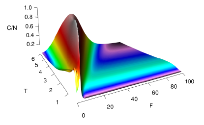
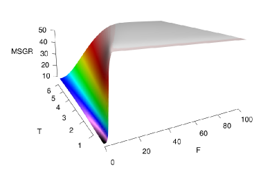
Figure 4: Plot of (a) the specific heat capacity of a trefoil knot with $N=70$ segments as a function of the rescaled force $\mathbf{F}$ and the temperature $\mathbf{T}$; (b) the mean square gyration radius of the trefoil. Both plots refer to the case of attractive forces $\varepsilon<0$.

Clearly we have that $\frac{H(X)}{T}=\frac{E(X)}{\mathbf{T}}$ and $Z(T,F)=Z(\mathbf{T},\mathbf{F})$. This justifies the computation of the observables using the rescaled units $\mathbf{T},\mathbf{F}$.

The results concerning the topological effects will be presented in Subsection III.1, while the effects related to size will be the subject of Subsection III.2. We restrict ourselves to the case $\mathbf{F}\geq 0$, because, due to the already mentioned symmetry of the Hamiltonian under the transformation $\mathbf{F},d_{z}\longrightarrow-\mathbf{F},-d_{z}$, the plots of the studied observables when $\mathbf{F}$ is negative are symmetric to those with $\mathbf{F}>0$ and do not provide any new information.

III.1 Topological effects of polymer knots

Three dimensional pictures are very helpful to illustrate the general features of the behavior of the analyzed knots. As a consequence, to start with, the three dimensional pictures of the specific heat capacity and gyration radius of a trefoil ($3_{1}$) knot with $70$ monomers will be discussed. The plot of these observables are displayed in Figs. 4 (a) and (b) in the range of parameters $0\leq\mathbf{F}\leq 100$ and $0.35\leq\mathbf{T}\leq 6$. Attractive interactions have been assumed, i. e. $\varepsilon<0$.

From Fig. 4 (a) it turns out that the trefoil polymer knot can be found in at least three different phases, which we identify as crystallite, expanded and stretched phases. At low temperatures and for weak stretching forces $F$, the knot is in the crystallite state. Its conformation is compact and ordered. With the rising of the temperature, this state undergoes a transition to the expanded state, characterized by a swollen and disordered conformation. This transition corresponds to the small peaks appearing approximately in the region in Fig. 4 (a) centered around $\mathbf{T}=1$ and such that $\mathbf{F}\sim 0$. When the strength of the tensile force grows, there is a transition from the crystallite state (at low temperatures) or from the expanded state (at high temperatures) to the stretched state. The broad peak characterizing the the heat capacity of the trefoil knot through the whole range of temperatures is caused by this transition. This conclusion is also confirmed by the results of the calculation of the mean square gyration radius displayed in Fig. 4 (b), which clearly shows that, for fixed $\mathbf{T}$ and $\mathbf{F}$, the growth rate of the gyration radius attains its maximum exactly in the position of the $\mathbf{T},\mathbf{F}$ plane in which the broad peak of the heat capacity is occurring. For example, when $\mathbf{T}=6$, the peak in the heat capacity is located at $\mathbf{F}=33.90$, see Fig. 4 (a). Looking at Fig. 4 (b), it is easy to realize that the coordinates of the maximum of the growth rate of the gyration radius are the same, i. e. $\mathbf{T}=6$ and $\mathbf{F}=33.90$. From Figs. 4 (a) and 5 it can also be observed that, as $\mathbf{T}$ decreases, the peak of the specific heat capacity becomes narrower and moves to lower values of $\mathbf{F}$. Correspondingly, the growth of the gyration radius near the transition is stronger at lower temperatures $\mathbf{T}$ and the point of maximum growth rate translates together with the peak of the heat capacity, see Fig. 4 (b). The narrowing of the peak is probably related to the fact that the stretching process is much more violent when the knot is in a compact state at low temperatures than at high temperatures, when the knot conformation is already swollen. On the other side, in order to stretch a polymer, the force $F$ needs to counteract the molecular motions of its monomers. With decreasing temperatures, the latter become weaker. This explains why the position of the peak in the heat capacity in the $\mathbf{T},\mathbf{F}$ plane moves along a curce such that $\left.\frac{d\mathbf{T}_{peak}(\mathbf{F})}{d\mathbf{F}}\right|_{F_{peak}}>0$ as shown clearly in Fig. 5. Of course, when the stretching force is so high that the polymer is already almost fully stretched, the stretching process gives negligible effects and the heat capacity, as well as the gyration radius, stop to change significantly.

Besides the two transitions described before, there is also a third and minor one with a peak in the heat capacity centered approximately along the line $\mathbf{T}=1$ in Fig. 4 (a). Its presence is clearly pointed out in the color shaded picture of Fig. 5. The existence of this peak is in agreement with the calculations of swetnam in the case of a figure-eight ($4_{1}$) knot. As a matter of fact, while the setups are different, we expect agreement of our results with those obtained in swetnam when the polymer is elongated. The minor peak persists even when the stretching force is very large. It corresponds to a transition occurring with the rise of the temperature when the knot passes from a stretched and compact state to a stretched and slightly more swollen state. In swetnam there are additional phase transitions taking place when the values of the force $F$ are negative. These are however related to compression, a phenomenon that is not reproducible by stretching and thus is not relevant in this work.

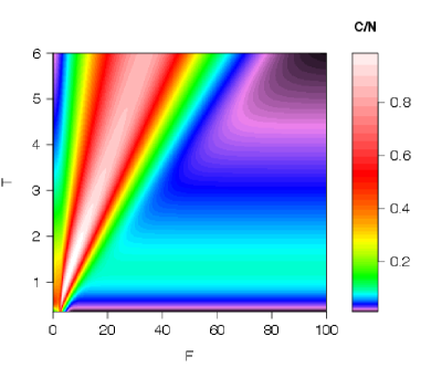
Figure 5: Color shaded picture of the heat capacity of a trefoil knot with $N=70$ segments in the $\mathbf{T},\mathbf{F}$ plane. In this figure it is possible to recognize a marked peak, corresponding to the transition from a compact to a stretched state. The peak becomes wider with increasing temperatures. Moreover, a secondary, smaller peak is shown (cyan area extending from $0.5\leq\mathbf{T}\leq 2$.

Let’s now go back to the topological effects. Figs. 4 and 5 suggest that, in a stretched polymer knot subjected to short range attractive forces, there are only two relevant phase transitions. The minor one, which is responsible for the smaller peak in Figs. 4 and 5, is probably a pseudo-phase transition and will be neglected in the following. The phase transition leading to the main peak of the heat capacity in Fig. 4 (a) can be observed in all studied knots at any temperature although, as we have seen, the maximum of the peak, as well as the maximum of the growth of the gyration radius, occur for different values of the stretching force $\mathbf{F}$, i. e. $\mathbf{T}_{peak}=\mathbf{T}_{peak}(\mathbf{F})$. As a consequence, we concentrate here on a given fixed temperature, for instance $\mathbf{T}=6$. The reason of this choice is the comparison with the results of Ref. swetnam . In that work, in fact, one of the two temperatures mainly used in the discussion was $\mathbf{T}=6$.

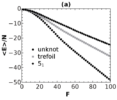
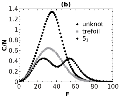
Figure 6: (a) The specific energy and (b) the heat capacity of the unknot $0_{1}$ (circles), the trefoil knot $3_{1}$ (rectangles) and the knot $5_{1}$ (diamonds). All knots have length of 50 lattice units. The normalized temperature is $\mathbf{T}=6$ and $\varepsilon<0$.

To study possible topological effects, in Fig. 6 the specific energy and heat capacity have been plotted in the case of the unknot ($0_{1}$), the trefoil and the knot $5_{1}$. All these knots have the same length $N=50$ and their monomers are subjected to attractive interactions ($\varepsilon<0$). The specific energy, see Fig. 6 (a), decreases with the growing of the stretching force. This is an expected result, as it is possible to realize looking at the rescaled Hamiltonian ${E}(X)$ of Eq. (13). Indeed, remembering that $\mbox{sign}(\varepsilon)=-1$ if the interactions are attractive, we have that both terms $m\mbox{sign}(\varepsilon)$ and $-Fd_{z}$ in the Hamiltonian are negative, while their absolute values grow when the strength of the stretching force is increasing. There are in fact two combined effects that contribute to lower the specific energy of the system. First of all, by stretching a swollen conformation, the number of contacts grows until a saturation value $m_{stretch}$ is reached. For example, $m_{stretch}=12$ for an unknot with $N=50$ segments. Secondly, under increasing tensile forces, the length $d_{z}$ converges in our setup to the maximum possible length $d_{z,max}$ of the knot. In the case of an unknot with $N=50$, it is easy to see that this length is $d_{z,max}=24$. All this explains the decrease of the specific energy mentioned before. For instance, when $\mathbf{F}=100$, we may suppose that the polymer is almost completely stretched, so that for an unknot the average value of the specific energy $\frac{\langle E\rangle}{N}\sim-\frac{12}{50}-\frac{100\cdot 24}{50}\sim-48.22$. Within a very good approximation, this is exactly the value of $\frac{\langle E\rangle}{N}$ for $\mathbf{F}=100$ obtained from our calculations, see in Fig. 6 (a) the plot of the specific energy for the unknot $0_{1}$.

The data concerning the specific heat capacity are displayed in Fig. 6 (b). It is possible to realize that the specific heat capacities of the unknot and the trefoil present respectively a single peak.

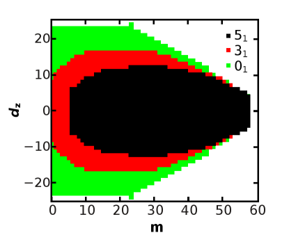
Figure 7: Accessible combinations ($m,d_{z}$) of the unknot $0_{1}$ (green rectangles), the trefoil $3_{1}$ (red rectangles) and the knot $5_{1}$ (black rectangles). All the knots consists of $50$ segments.

As we have already discussed, this peak can be interpreted as the result of the transition from an expanded phase to a stretched phase. The case of the knot $5_{1}$ is exceptional because two equivalent peaks are observed. The presence of this additional peak is almost certainly a consequence of the fact that in a knot $5_{1}$ with only $50$ segments the monomers are very close to each other and are thus strongly interacting. In this situation, the topological effects are enhanced. To convince ourselves about that, it is sufficient to remember that the minimum number of segments necessary to construct a knot $5_{1}$ on a simple cubic lattice is $34$. In comparison, the simpler knot $3_{1}$ and the unknot $0_{1}$ have a minimum length of $4$ and $24$ lattice basic units respectively mini . It is thus expected that in such a complex and short knot like a $5_{1}$ with $N=50$ segments the expansion process is complicated by the topological constraints. This fact is also confirmed by Fig. 7, which clearly shows that the number of possible energy states of a $5_{1}$ knot, determined by the allowed values of the parameters $m$ and $d_{z}$ on the lattice, is definitely less than the analogous number in the case of a trefoil or an unknot of the same length. In conclusion, the appearance of the double peaks of $5_{1}$ is a topological effect appearing due to the limitations of the knot $5_{1}$ in accessing new energy states during its expansion process. As a counter-check, we have computed the specific heat capacity of a longer knot $5_{1}$ with $N=70$. The result is shown in Fig. 8 (b). As it is possible to see, now only a single peak is observed.

By increasing the number of segments, more complicated knots with higher minimal crossing numbers can be formed. In Fig. 8 we present for instance the plots of the specific energy and heat capacity for the knots $0_{1},3_{1},4_{1},5_{1},5_{2}$ and $7_{1}$ with $N=70$.

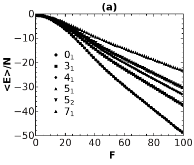
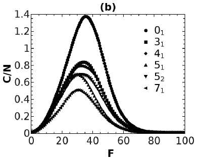
Figure 8: (a) The specific energy and (b) the heat capacity of the unknot $0_{1}$ (circles), the trefoil knot $3_{1}$ (rectangles), the figure-eight $4_{1}$ (diamonds), the knot $5_{1}$ (up triangle), the knot $5_{2}$ (down triangle) and the knot $7_{1}$ (left triangle). All knots have 70 segments. The normalized temperature is $\mathbf{T}=6$ and $\varepsilon<0$.

It is clear that topology affects the thermal properties of these polymer knots. As shown in Figs. 6 and 8, in fact, in the attractive case the increasing of the knot complexity results in a decrease of the specific energy and the heat capacity. The reason is that more complex knots tend to have more compact conformations, which have in the average a higher number of contacts. The presence of more contacts lowers the average energy of each monomer if the interactions are attractive, so that in turn the specific energy decreases. The fact that with increasing topological complexity knots have more compact conformations has been shown in the absence of stretching in Ref. yzff2013 . This conclusion is also confirmed when stretching is applied by the data on the mean square gyration radii of the considered knots, see Fig. 9.

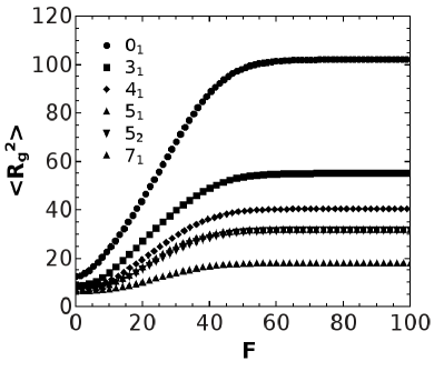
Figure 9: The mean square gyration radius of the unknot $0_{1}$ (circles), the trefoil knot $3_{1}$ (rectangles), the figure-eight $4_{1}$ (diamonds), the knot $5_{1}$ (up triangle), the knot $5_{2}$ (down triangle) and the knot $7_{1}$ (left triangle). All knots have 70 segments. The normalized temperature is $\mathbf{T}=6$ and $\varepsilon<0$.

In particular, the gyration radii $\langle R_{G}^{2}\rangle(T,F)$ satisfy the inequality

$$\langle R_{G}^{2}\rangle_{0_{1}}>\langle R_{G}^{2}\rangle_{3_{1}}>\langle R_{G}^{2}\rangle_{4_{1}}>\langle R_{G}^{2}\rangle_{5_{1}}=\langle R_{G}^{2}\rangle_{5_{2}}>\langle R_{G}^{2}\rangle_{7_{1}}$$ (14)

independently if the interactions are attractive – case shown in Fig 9 – or repulsive. Let us notice that the knots $5_{1}$ and $5_{2}$ have more or less the same average gyration radius. This suggests that knots with the same minimum crossing number have a similar behavior.

Looking at the plots of the specific energy and heat capacity at fixed temperature, in particular at Figs. 10 and 11, where the insets show in details the behavior when $\mathbf{F}$ is small, three regimes may be distinguished in the range of forces $0\leq\mathbf{F}\leq 100$. In these regimes the thermal properties of a polymer knot are profoundly different:

1. When $\mathbf{F}<<\mathbf{F}_{peak}$, the studied system is below the threshold in which the transition to the stretched phase is occurring. In this region the decreasing of the specific energy as the stretching force increases is relatively slow. Moreover, the heat capacity is slowly increasing with increasing values of $\mathbf{F}$.

2. Near $\mathbf{F}=\mathbf{F}_{peak}$ the system undergoes the transition from the expanded state to the stretched state. With respect to the previous regime, the decrease of the specific energy with increasing values of $F$ is more marked. The peak with the maximum value of the heat capacity is located in this region.

3. After the phase transition has been completed, the system finds itself in the stretched phase, which is characterized by large values of the tensile force $F$. As a consequence, the mechanical term $-Fd_{z}$ becomes dominant in the Hamiltonian of Eq. (1) and the specific energy of the system linearly decreases proportionally to $\mathbf{F}$. The heat capacity goes instead to zero because when the knot conformation is already almost stretched, any further stretching becomes difficult .

As it is possible to notice from Fig. 8 (b), with increasing knot complexity the height of the peak in the heat capacity is decreasing and its width is getting narrower. This is because in more complex knots the stretching process is hindered by the topological constraints, which require more turns in the polymer trajectory than in simpler knots. As a result, the more complex the knot, the closer to each other stay the monomers.

III.2 Size effects of polymer knots

To study the size effects of polymers, we consider in this Subsection polymers of the same knot type (the trefoil knot $3_{1}$) but different lengths. Fig. 10 shows the results of the calculations of the specific energy and heat capacity of a $3_{1}$ knot in the case of attractive monomer-monomer interactions at $\mathbf{T}=6$. The most striking effect which can be related to the length of the knot can be found in the linear decay of the specific energy in Fig. 10. In the third regime discussed in the previous Subsection, this decay is proportional to $F$ and, remarkably, it becomes steeper as the knot length $N$ increases. The reason for which the specific energy of longer knots should be less than that of shorter polymers as observed in Fig. 10 is not entirely intuitive, but can be explained as follows. In the stretched phase the mechanical term $-\mathbf{F}d_{z}=-\frac{Fd_{z}}{|\varepsilon|}$ becomes dominant in the rescaled Hamiltonian $E(X)$ of Eq. (13). Obviously, if the rescaled force $\mathbf{F}$ is fixed, the decrease of the specific energy can only depend on the value of $\frac{d_{z}}{N}$ and on the topology of the considered knot. Of course, the maximum value of $\frac{d_{z}}{N}$ is obtained when the topology is that of the unknot. Indeed, if a trefoil is stretched with the same force $\mathbf{F}$ as an unknot of the same length $N$, then the obtained average value of the ratio $d_{z}^{3_{1}}(N)/N$ will be lower than that of an unknot, i. e.: $\frac{d_{z}^{3_{1}}(N)}{N}<\frac{d_{z}^{0_{1}}(N)}{N}$. This is due to the fact that in the trajectory of the trefoil knot a part of the trajectory cannot be stretched, because it contains the turns that are necessary in order to satisfy the topology requirements. At this point we recall that the effects of topology are supposed to eventually fade out when the length of a knot becomes infinite. In this limit, the portion of the trajectory that is bending and twisting due to the topological constraints becomes irrelevant in comparison with the rest of the knot and the difference between the behavior of an arbitrary knot and the unknot disappears. In other words, the topological effects fade out when the number of segments $N$ is increasing. In our case, this implies that the ratio $d_{z}^{3_{1}}/N$ should grow with increasing values of $N$ in such a way that, eventually, we have that $\lim_{N\to\infty}\frac{d_{z}^{3_{1}}(N)}{N}=\frac{d_{z}^{0_{1}}(N)}{N}$. This growth of the ratio $\frac{d_{z}^{3_{1}}(N)}{N}$ with $N$ is exactly what is observed in Fig. 10 and explains the faster decrease of the specific energy, because it is the reason for which the dominating term $-\mathbf{F}\frac{d_{z}(N)}{N}$ in the Hamiltonian decreases with $N$.

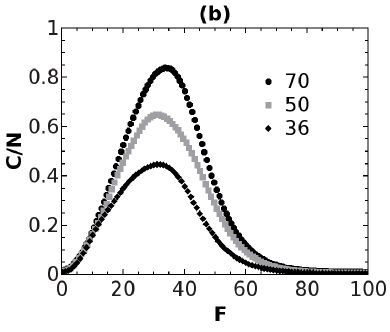
Figure 10: (a) The specific energy and (b) the heat capacity of trefoil knots $3_{1}$ with lengths $N=36$ (diamonds), $N=50$ (rectangles) and $N=70$ (circles). The normalized temperature is $\mathbf{T}=6$ and $\varepsilon<0$. The inset in (a) shows the details of the behavior of the specific energy at weak tensile forces.

Regarding the heat capacity, we can see in Fig. 10 (b) that there is only one peak in the whole studied interval of forces. The interpretation of this peak is the same as in the previous Subsection. In the present case, the peak in the heat capacity corresponds to the transition of the trefoil knot from an expanded state to a stretched state. Similar phase transitions have already been observed in unknots, see swetnam . It is worth to note that the peak is higher in the case of longer polymer and its position is slightly shifted toward bigger values of $\mathbf{F}$ as $N$ increases. These are finite size effects that are very well documented in the polymer literature, see for instance finitesizeeffects . Analogous considerations can be made when the interactions are repulsive. This case is displayed in Fig. 11.

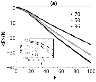
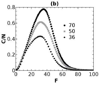
Figure 11: (a) The specific energy and (b) the heat capacity of a trefoil knot $3_{1}$ considered at different lengths $N=36$ (diamonds), $N=50$ (rectangles) and $N=70$ (circles). The normalized temperature is $\mathbf{T}=6$ and the interactions are repulsive ($\varepsilon>0$). The inset in (a) shows the details of the behavior of the specific energy at weak tensile forces.

The main difference from knots subjected to attractive interactions is that in the region in which the tensile forces are very weak, the specific energy is always positive and not negative as in the case $\varepsilon<0$. The reason is that, for small values of $F$, the repulsive term $m\varepsilon$, which is always positive apart from the rare conformations with no contacts at all, is dominating the Hamiltonian (1). Nonetheless, independently of the sign of $\varepsilon$, the specific energy of the trefoil knot decreases monotonically in the whole $\mathbf{F}$ region, see the insets in Figs. 10 (a) when $\varepsilon<0$ and 11 (a) when $\varepsilon>0$. Despite the fact that the behavior of the heat capacity in Fig. 11 (b) is very similar to that in which the interactions are attractive, see Fig. 10 (b), when $\varepsilon<0$, the height of the peak in the latter case is slightly smaller. This is due to the contribution of the contact term in the Hamiltonian. Also in the phase transition from crystallites to expanded states without stretching studied in Refs. yzff and yzff2013 , the peak of the heat capacity is higher when the interactions are attractive. For the same reason, the values of $\langle R_{G}^{2}\rangle$ at $\varepsilon<0$ are slightly smaller than those measured when $\varepsilon>0$, see Figs. 12 (a) and (b).

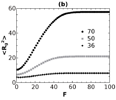
Figure 12: The mean square gyration radius of a trefoil knot $3_{1}$ considered at different lengths $N=36$ (diamonds), $N=50$ (rectangles) and $N=70$ (circles). In (a) the case of attractive interactions ($\varepsilon<0$) is displayed. In (b) the interactions are repulsive ($\varepsilon>0$). The normalized temperature is $\mathbf{T}=6$.

In both cases of $\varepsilon<0$ (Fig. 12 (a)) and $\varepsilon>0$ (Fig. 12 (b)), the gyration radius starts to grow abruptly more or less at the point $\mathbf{F}=\mathbf{F}_{peak}$ where the peak in the heat capacity is appearing. This similarity of behavior is due to the that we are considering here the phase transition from the expanded to the stretched phase, in which the mechanical term $-\mathbf{F}d_{z}$ is predominant. In this regime, the repulsive interactions give a negligible contribution to the average specific energy. Only when $\mathbf{F}$ is small, the contact interactions become relevant. In a neighborhood of $\mathbf{F}=0$, indeed, the values of $\langle R_{g}^{2}\rangle$ in the case of attractive interactions are always smaller than those obtained when the monomers repel themselves.

IV Conclusions

In this work we have studied the mechanical properties of polymer knots under stretching by an tensile force $F$ directed along the $z-$axis. The force has been applied to one point of the knot, while another point has been anchored to a lattice site. A picture of the system can be found in Fig. 1. Short polymers with a length up to $N=70$ lattice units have been considered. In short polymers like these, the effects due to the topology of the knot are particularly evident. Moreover, for short polymers it is relatively easy to sample all the accessible energy states without the need of introducting cutoffs in the energy range. In performing the sampling the Wang-Landau algorithm of Ref. newwl has been proved to be very convenient. The three dimensional pictures of Figs. 4 (a) and (b) show the general trend in the behavior of short polymer knots under stretching. Besides the expanded and crystallite phases, there is still also a stretched phase. When tensile forces are weak, the knot can be found in the compact or expanded state depending on the temperature. The transition from these states to the stretched phase takes place at any temperature. In the case of a trefoil knot at high temperatures ($\mathbf{T}=6$), the peak of the heat capacity during the transition is located on the $\mathbf{F}-$axis at $\mathbf{F}_{peak}\sim 35$, see Figs. 10 and 11. With decreasing temperatures also the values of $\mathbf{F}_{peak}$ decrease, meaning that it is easier to stretch a very compact knot at low temperatures than a swollen one at high temperatures, where strong thermal fluctuations try to bring back the knot to those conformations that maximize the entropy of the system. When the temperature is very low, the stretching process is abrupt and gives rise to a sharp peak in the heat capacity, see Fig. 4 (a). Besides the decreasing of the temperature, there are other factors that shift $\mathbf{F}_{peak}$ to lower values, namely the increasing of the topological complexity of the knot (see Fig. 8 (a)) and the decreasing of the polymer size (see Figs. 10 and 11). Moreover, almost entirely stretched knots can still pass from a compact state to the expanded state with rising temperatures. This phenomenon causes the appearance of the minor peak in Fig. 5.

Topological effects are more visible when polymers are very short, as it is proved by the presence of the double peak of the heat capacity of the knot $5_{1}$ with $N=50$ in Fig. 6 (b). Surprisingly, these effects fade out rapidly with increasing knot sizes. For example, the slope of the energy decay of the trefoil knot with $N=70$ of Fig. 10 (a) is almost equal to the slope of the unknot with $N=70$ of 8 (a). Moreover, in the stretched regime, where the mechanical term becomes dominant in the Hamiltonian (1), the behavior of knots subjected to repulsive or attractive forces is the same apart from small deviations as it is expected.

Our work can be generalised under several aspects. First of all, we limited ourselves to the Hamiltonian of Eq. (1) even if there are no obstacles to to extend our procedure to describe more realistic polymer systems, for instance by considering the rigidity of polymer knots or adding more complex potentials considering the rigidity of polymer knots. This will be our next research task. We also plan to apply our current method to proteins which have knotted native structures. We hope to be able to report on these new developments very soon.

- (1) P. Virnau, L. A. Mirny and M. Kardar, PLoS comput. Biol. 2 (2006), e122.
- (2) A. L. Mallam and S. E. Jackson, Nature chemical biology 8 (2012), 147.
- (3) J. Arsuaga, M. Vazquez, S. Trigueros, D. W. Sumners and J. Roca, PNAS 99 (2002), 5373.
- (4) M. L. Mansfield, Nat. Struct. Biol. 1 (1994), 213.
- (5) Daniel Bo ̵̈linger, Joanna I. Sulkowska, Hsiao-Ping Hsu, Leonid A. Mirny, Mehran Kardar, Jose N. Onuchic and Peter Virnau, PLoS comput. Biol. 6 (2010), e1000731.
- (6) C. O. Dietrich-Buchecker and J. P. Sauvage, Angew. Chem. Int. Ed. Engl. 28 (1989), 189.
- (7) M. Schappacher and A. Deffieux, Ang. Chemie 48 (2009), 5930.
- (8) Y. Ohta, Y. Kushida, Y. Matsushita and A. Takano, Polymer 50 (5) (2009), 1297.
- (9) Y. Ohta, M. Nakamura, Y. Matsushita and A. Takano, Polymer 53 (2012), 466.
- (10) Y. Arai, R. Yasuda, K.-I. Akashi, Y. Harada, H. Miyata, K. Kinosita Jr and H. Itoh, Nature 399 (1999), 446.
- (11) A. M. Saitta, P. D. Soper, E. Wasserman and M. L. Klein, Nature 399 (1999), 46.
- (12) S. D. Levene, C. Donahue, T. C. Boles and N. R. Cozzarelli, Biophys. J. 69 (1995), 1036.
- (13) J. Arsuaga, M. Vazquez, P. M. Guirk, S. Trigueros. D. W. Sumners and J. Roca, PNAS 102 (2005), 9165.
- (14) P. F. N. Faisca, R. D. M. Travasso, T. Charters, A. Nunes, M. Cieplak, The folding of knotted proteins: Insights from lattice simulations, Physical Biology 7 (1) (2010), 016009.
- (15) J. I. Sułkowska and M. Cieplak, Biophys. J. 94 (2008), 6.
- (16) J. Elbaz, Z. Wang, F. Wang and I. Wilner, Angew. Chem. Int. Ed. 51 (2012), 2349.
- (17) J. Vinograd, J. Lebowitz, R. Radloff, R. Watson and P. Laipis, Proc Natl Acad Sci USA 53 (1965), 1104.
- (18) A. Narros, A. J. Moreno and C. N. Likos, Macromolecules 46 (9) (2013), 3654.
- (19) C. Weber, P. D. L. Rios, G. Dietler and A. Stasiak, J. Phys. Condens. Matter 18 (2006), S161.
- (20) P. Serna, G. Bunin and A. Nahum Phys. Rev. Lett. 115 (2015), 228303.
- (21) M. Kapnistos, M. Lang, D. Vlassopoulos, W. Pyckhout-Hintzen, D. Richter, D. Cho, T. Chang and M. Rubinstein, Nature 7 (2008), 997.
- (22) M. D. Hossain, D. Valade, Z. Jia and M. J. Monteiro, Polymer Chemistry 3 (2012), 2986.
- (23) M. D. Hossain, Synthesis of Cyclic Macromolecular Architectures, PhD thesis, University of Queensland, 2014.
- (24) M. Caraglio, C. Micheletti and E. Orlandini, Phys. Rev. Lett. 115 (2015), 188301.
- (25) F. Ferrari and I. Lazzizzera, Nucl. Phys. B 559 (3) (1999), 673.
- (26) F. Ferrari, Annalen der Physik (Leipzig) 11 (2002) 4, 255.
- (27) F. Ferrari and I. Lazzizzera, Phys. Lett. B 444 (1998), 167.
- (28) F. Ferrari, H. Kleinert and I. Lazzizzera, Eur. Phys. J B 18 (2000), 645.
- (29) F. Ferrari, M. R. Pia̧tek and Y. Zhao, J. Phys. A: Mathematical and Theoretical, 48 (2015), 275402, arXiv: 1411.6429.
- (30) C. M. Rohwer and K. K. Müller-Nedebock, J. Stat. Phys. bf 159 (2015), 120.
- (31) C. Zhou and J. Su, Phys. Rev. E 78 (2008), 046705.
- (32) F. Wang and D. P. Landau, Phys. Rev. Lett. 86 (2001), 2050; F. Wang and D. P. Landau, Phys. Rev. E 64 (2001), 056101.
- (33) P. N. Vorontsov-Velyaminov, N. A. Volkov and A. A. Yurchenko, J. Phys. A: Math. Gen. 37 (2004), 1573.
- (34) A. Swetnam, C. Brett and M. P. Allen, Phys. Rev. E 85 (2012), 031804.
- (35) Y. Zhao and F. Ferrari, JSTAT J. Stat. Mech. (2012), P11022.
- (36) Y. Zhao and F. ferrari, J. Stat. Mech. (2013), P10010.
- (37) N. Madras, A. Orlistsky and L. A. Shepp, J. Stat. Phys. 58 (1990), 159.
- (38) R. E. Belardinelli and V. D. Pereyra, Phys. Rev. E 75 (2007), 046701.
- (39) M. P. Taylor, W. Paul and K. Binder, J. Chem. Phys. 131 (2009), 114907.
- (40) Y. Zhao and F. Ferrari, Acta Physica Polonica B 44 (2013), 1193.
- (41) Vogel T, Bachmann M and Janke W, 2007 Phys. Rev. E 76 061803
- (42) A. Swetnam and M. P. Allen, J. Comput. Chem. 32 (2011), 816.
- (43) R. Scharein, K. Ishihara, J. Arsuaga, Y. Diao, K. Shimokawa and M. Vazquez, J. Phys. A: Math. Theor. 42 (2009), 475006.
- (44) J. P. K. Doye, R. P. Sear and D. Frenkel, Jour. Chem. Phys. 108 (1998), 2134.