Noisy threshold in neuronal models: connections with the noisy leaky integrate-and-fire model.

Abstract

Providing an analytical treatment to the stochastic feature of neurons’ dynamics is one of the current biggest challenges in mathematical biology. The noisy leaky integrate-and-fire model and its associated Fokker-Planck equation are probably the most popular way to deal with neural variability. Another well-known formalism is the escape-rate model: a model giving the probability that a neuron fires at a certain time knowing the time elapsed since its last action potential. This model leads to a so-called age-structured system, a partial differential equation with non-local boundary condition famous in the field of population dynamics, where the age of a neuron is the amount of time passed by since its previous spike. In this theoretical paper, we investigate the mathematical connection between the two formalisms. We shall derive an integral transform of the solution to the age-structured model into the solution of the Fokker-Planck equation. This integral transform highlights the link between the two stochastic processes. As far as we know, an explicit mathematical correspondence between the two solutions has not been introduced until now.

1 Introduction

Neurons are strongly noisy. They never respond in the same way under repeated exposure to identical stimuli and it is difficult for theoreticians to apply the correct analytical treatment in order to express this variability. Two distinct sources of noise are usually mentioned: external and internal noiseNS . While the external source of noise usually refers to the random fluctuations attributed to the environment of the neurons, the internal source is mainly imputed to the probabilistic nature of the chemical reactions governing the firing process of neurons. More precisely, noise is present because a neuron is bombarded by thousands of synaptic inputs, and also due to the randomness in the openings and closings of the ion channels underlying action potentials andre01 .

The noisy leaky integrate-and-fire (NLIF) model is a mathematical model that takes into account the stochastic features of neurons Burkitt . The model is preferred by theoreticians since it can be seen as a simplification of the bio-physiological Hodgkin-Huxley model HH , which is sufficiently detailed to allow a qualitative comparison with physical data obtained via intracranial recording Izi (see also naud for a recent discussion about the quality of the neural modeling). Nonetheless, despite its apparent simplicity, many questions regarding its dynamics remain open.

By definition, the NLIF model describes a stochastic process, which is given by a Langevin equation plus a discontinuous reset mechanism to mimic the onset of the action potential (see Burkitt and Izi ). Starting with the Langevin equation, one can write the well-known associated Fokker-Planck (FP) equation Gardiner , that gives the evolution in time of the density probability to find a neuron’s membrane potential in a certain voltage value longtin01 .

Let us remind that, in mathematical neuroscience, the concept of probability density function has already a long history, as it can be seen in rinzel , abbott , and it is used in a variety of contexts. Indeed, assuming the number of neurons to be infinitely large, one can write the so-called thermodynamics’ mean field equation, where the effect of the whole network on any given neuron is approximated by a single averaged effect. Under some assumptions and approximations, the equation takes the form of a nonlinear FP equation. It is in particular pertinent for the simulation of large sparsely connected populations of neurons sirovich , nykamp , us . Furthermore, this density approach has brought an important added value on the theoretical understanding of synchronization and brain rhythms. Particularly, this approach has been successfully used to understand synchronization caused by recurrent excitation DH , DH01 , carillo01 , by delayed inhibition feedback BH01 , by both recurrent excitation and inhibition B02 and by gap junction brunel01 . On a similar trend, it has been used to study the occurrence of the neural cascade cascade01 , cascade02 and the emergence of self criticality critical with synaptic adaptation.

In this paper, we do not investigate the effect of interactions among neurons, but focus on the analytical treatment of neural noise. NLIF model is a popular way to deal with the stochastic aspect of neurons, another way is the escape-rate model plesser , gerstner . The main difference between the two approaches consists in the treatment of noise; while in the NLIF model the noise acts on the trajectories, the escape rate model considers deterministic trajectories and the noise is present in expressing the variability of firings that is modeled in the form of a hazard function. Therefore, the noisy trajectories with fixed threshold are replaced by deterministic trajectories with noisy thresholds. In the equivalent description of the NLIF model as a FP equation with absorbing boundary condition at the firing threshold, the noise is expressed by the diffusion term of the FP equation; it has been shown in plesser that, in the subthreshold regime, the integrate and fire model with stochastic input (diffusive noise) can be mapped onto an escape rate model with a certain escape rate. Starting from this, the equivalence of the FP equation with escape noise and a partial differential equation that describes the evolutions of refractory densities has been shown gerstner ; the last equation is strikingly similar to those of the well-known age-structured (AS) models and it gives the evolution in time of the refractory densities with respect to their refractory state, which is in fact the time elapsed since the last firing. To underline the above mentioned similarity, we will refer to this variable in this paper as age. Age structure in a neural context has been also discussed in perthame03 .

In our paper, we shall prove that the solution to the AS system can be transformed via an integral transform into the solution to the FP equation associated to the NLIF model. The kernel of the integral transform will involve in particular the notion of survivor function g2000 , gerstner . In renewal theory, the hazard is known also as the age dependent death rate and expresses the rate of decay of the survivor function cox . The concept of time dependent interspike interval (ISI) distribution and corresponding survivor function has been considered later G95 .

In the neuroscience context, the survivor function, which was introduced initially to describe the probability of a particle to reach a given target, will give the probability for a neuron to ”survive” without firing. We refer again for more about these considerations to gerstner , and further analysis on these functions and the related first passage time problem in the neural context can be found in the review BN . First passage time problem in cellular domains has been investigated in schuss and holcman .

There is a strong advantage in using an AS formalism: the AS systems have been thoroughly investigated in the last decades, and many qualitative results of the various forms of AS population models have been obtained. By proving an equivalence between a membrane potential density model and an AS model, we will be in position to obtain insights of the qualitative behavior of the population density function such as long time behavior, stability, bifurcation points, and so on.

The paper is structured as follows: we remind in the first two sections the NLIF model and its associated FP equation, and we present some simulations of the models. Next, some considerations about the survivor function, the interspike interval distribution and the first passage time problem are presented. We introduce in the following the stochastic threshold model and the corresponding AS system. We prove our main theoretical results in the last two sections: first we establish in Proposition 1 an integral correspondence between its solution and the solution to FP equation. We also consider the stationary case, and show that, by our integral transform, we obtain an expression of the corresponding stationary solution which verifies the stationary FP equation. Last, we show the asymptotic convergence of the solution to FP system to the solution of the stationary system defined through our transform. The existence of an inverse transform to the one introduced here as well as extensions of the problem to the case of time-dependent parameters of the systems are subject to our further investigations .

Before getting started, let us summarize in Table 1 the main mathematical notations and their associated biophysiological meaning used throughout this document.

Notation	Biophysiological interpretation
$v(t)$	Neuron’s membrane potential
$v_{r}$	Reset potential
$\mu$	Bias current
$\sigma$	Noise intensity
$p(t,v)$	Population density with respect to potential
$r(t)$	Neuron’s firing rate
$a(t)$	Neuron’s age, i.e. time elapsed since the last spike
$q(a,v)$	Joint probability density of the membrane’s potential and neuron’s age
$ISI(a)$	First passage time
$S(a)$	Age dependent death rate
$n(t,a)$	Population density for the age-structured model

Table 1: Main notations used throughout this paper and their biophysiological interpretations

2 The noisy leaky integrate and fire model

The NLIF model is a well known model in the field of computational neuroscience Izi . The model consists in an ordinary differential equation describing the subthreshold dynamics of a single neuron membrane’s potential and the onset of an action potential described by a reset mechanism: a spike occurs whenever a given threshold $V_{T}$ is reached by the membrane potential variable $V$. Whenever the firing threshold is reached, it is considered that a spike has been fired and the membrane potential is instantaneously reset to a given value $V_{R}$. The dynamics of the subthreshold potentials are given by

$$\tau\frac{d}{dt}V(t)=-g(V(t)-V_{L})+\eta(t),\\$$

where $V(t)$ is the membrane potential at time $t$, $\tau$ is the membrane capacitance, $g$ - the leak conductance, $V_{L}$ - the reversal potential and $\eta(t)$ - a gaussian white noise, see B01 and abbott01 for the history of the model, Burkitt for a recent review and see Izi for other spiking models. In what follows, we will use a normalized version of the above equation, i.e. we define $\mu$ as the bias current and $v$ the membrane’s potential which will be given by

$$\mu=\frac{V_{L}}{V_{T}},\quad v=\dfrac{V}{V_{T}},\quad v_{r}=\frac{V_{R}}{V_{T}}.$$

After rescaling the time in units of the membrane constant $g/\tau$, the normalized model reads

$$\left\{\begin{array}[]{l}\frac{d}{dt}v(t)=\mu-v(t)+\xi(t)\\ \text{If}\quad v>1\quad\text{then}\quad v=v_{r}.\end{array}\right.$$ (1)

Again, $\xi(t)$ is a Gaussian white noise stochastic process with intensity $\sigma$:

$$\langle\xi(t)\rangle=0,\quad\langle\xi(t)\xi(t^{\prime})\rangle=\sigma\delta(t-t^{\prime}).$$

In Fig. 1, a simulation of the neuron model (1) is presented. The three panels correspond to the same simulation with different level of noise. As expected, when the stochastic coefficient is increased, the corresponding dynamics become much more irregular. Note that for $\mu$ small enough, the equilibrium of the membrane potential will be located under the threshold. In this situation, the neuron will fire only due to the stochastic Brownian motion. We refer to this situation as to a subthreshold regime. In a real-world setting, such situation appears in a balanced neural network for instance, when the excitatory and inhibitory pre-synaptic inputs cancel out.

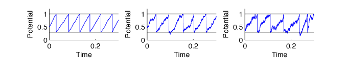
Figure 1: Simulation of the neuron model (1) for different values of the noise coefficient. The parameters of the simulation are: $v_{r}=0.3$, $\mu=20$, and $\sigma=0.1$ for the first simulation, $\sigma=0.4$ for the second simulation, $\sigma=0.6$ for the third simulation.

3 The population density function (Fokker-Planck formalism)

Considering a population of neurons that are individually described by the stochastic equation (1), the evolution of the population density function has been proven to satisfy the FP equation. We remind that the FP equation has been used in two different contexts in mathematical neuroscience: to model the evolution of both probability density function and population density function. For more considerations about the link between the two approaches we refer to nykamp , knight , K2000 , BH01 .

In this paper we shall use both formalisms: we shall consider a density of neurons characterized by a population density function, denoted here by $p(t,v)$, which satisfies the FP equation, and each neuron of the given population has the evolution of the potential of the membrane given by the NLIF model. Then, the probability density function of each neuron to be at a certain voltage at a given time will be described by the same FP equation Gardiner , this time considered only in an inter-spike interval, as we shall see in the next section.

This equation is a conservation law taking into account three phenomena modeled by: a drift term due to the continuous evolution in the NLIF model, a diffusion term due to the noise and a term due to the reset to $v_{r}$ right after the firing process. Let $r(t)$ be the firing rate of the population, i.e. the flux through the threshold. Then, the dynamics of the population density $p(t,v)$ is:

$$\frac{\partial}{\partial t}p(t,v)+\overbrace{\frac{\partial}{\partial v}[(\mu-v)p(t,v)]}^{\text{Drift}}-\overbrace{\frac{\sigma^{2}}{2}\frac{\partial^{2}}{\partial v^{2}}p(t,v)}^{\text{Diffusion}}=\overbrace{\delta(v-v_{r})r(t)}^{\text{Reset}}.\quad$$ (2)

We show in Fig. 2 a schematic representation of the state space for the FP equation (2).

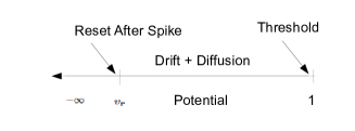
Figure 2: Schematic representation of the state space for the FP equation (2).

Because a neuron reaching the threshold fires an action potential and is instantaneously reset to $v_{r}$, we impose an absorbing condition at the threshold (gillespie ), namely

$$p(t,1)=0,\forall t\geq 0.$$ (3)

Usually, a reflecting boundary is imposed at $v=-\infty$ in order to assure the conservation property

$$\lim\limits_{v\to-\infty}(-\mu+v)p(t,v)+\frac{\sigma^{2}}{2}\frac{\partial}{\partial v}p(t,v)=0,\forall t\geq 0.$$ (4)

Of course, an initial distribution of the membrane potential is taken as a given function:

$$p(0,v)=p_{0}(v),\quad v\in(-\infty,1].$$ (5)

As previously said, the firing rate $r(t)$ is defined as the flux at the threshold and, due to the boundary condition for the population density function in this value, is given by

$$r(t)=-\frac{\sigma^{2}}{2}\frac{\partial}{\partial v}p(t,1).$$ (6)

Using the boundary condition and the expression of $r(t)$ given by (6), one can easily check the conservation property of the equation (2) by directly integrating it on the interval $(-\infty,1)$, so that, if the initial condition satisfies

$$\int_{-\infty}^{1}p_{0}(v)\,dv=1,$$ (7)

then the solution to (2)-(6) necessarily satisfies the normalization condition

$$\int_{-\infty}^{1}p(t,w)\,dw=1.$$ (8)

Despite its ”weird” singular source term, the existence of a solution to the above model has been proved in carrillo02 . The FP equation can be written as a Stephan problem and an implicit solution can be given in the form of an integral equation. Note that in the literature, the equation (2) is often exposed in terms of a conservation law. In this setting, the flux that we denote $\mathfrak{J}(t,v)$ is defined as

$$-\mathfrak{J}(t,v)=(-\mu+v)p(t,v)+\frac{\sigma^{2}}{2}\frac{\partial}{\partial v}p(t,v).$$

Therefore, the evolution in time of the density function $p$ is given by

$$\frac{\partial}{\partial t}p(t,v)=-\frac{\partial}{\partial v}\mathfrak{J}(t,v).$$

In this formulation, the singular source term that appears in (2) can be seen as a flux discontinuity, see B02 for instance,

$$\lim\limits_{v\to v_{r}^{+}}\mathfrak{J}(t,v)-\lim\limits_{v\to v_{r}^{-}}\mathfrak{J}(t,v)=\mathfrak{J}(t,1).$$

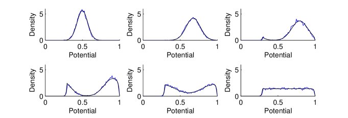
Figure 3: Simulations of the FP equation (2)-(6) and of the stochastic process (1): black curve for the FP equation, blue curve for the stochastic process. A gaussian was taken as initial condition; the parameters of the simulation are: $v_{r}=0.3$, $\mu=20$, $\sigma=0.4$. The plots show the evolution in time of the solution at $t=0$, $t=0.1$, $t=0.3$, $t=0.5$, $t=0.7$, $t=7$.

We present in Fig 3 a simulation of the FP model (2)-(6). The numerical results are compared with Monte Carlo simulations for the stochastic NLIF model (1). In Fig 3, the black curve corresponds to the FP equation (2)-(6) and the blue curve to the stochastic process (1). A Gaussian was taken as initial condition (see the first panel of Fig. 3). Under the drift and the diffusion effects, the density function gives a non zero flux at the threshold. This flux is reset to $v_{r}$ according to the reset process. This effect can be seen clearly in the third panel of the simulation presented in Fig. 3. Asymptotically the solution reaches a stationary density. The steady state is shown in the last panel of Fig. 3. Note that the stationary state can be easily computed (we remind its expression later in the text). One can show the convergence of the solution towards the stationary density using the general relative entropy principle.

In Fig. 4 a comparison of the firing rate (6) computed via the FP formalism (2) and via the stochastic model (1) is represented. Again the blue curve is obtained by direct simulations of the stochastic process (1), and the black curve corresponds to the simulations of the FP model (2)-(6). To be more precise, we also show a raster plot depicting the spike timing of the neurons for each simulation run. In the three different simulations that we present, we have varied the drift term $\mu$.

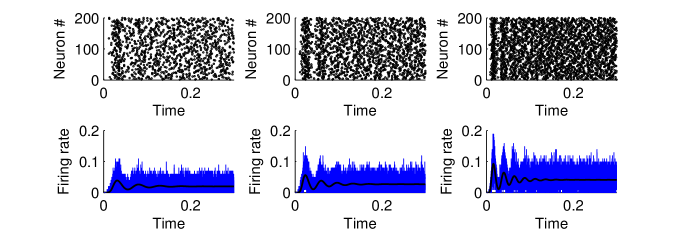
Figure 4: Simulation of the firing rate of the neuron (6) via the FP formalism (2)-(6), black curve, and the stochastic process (1), blue curve. The parameters of the simulation are: $v_{r}=0.3$, $\mu=15$ and $\sigma=0.4$ for the first simulation, $\mu=20$ and $\sigma=0.4$ for the second simulation and $\mu=30$ and $\sigma=0.4$ for the third simulation. We also show the raster plot depicting the spike timing of $200$ neurons.

The stationary state of the FP equation is known from decades. A straightforward computation shows that the steady state $p_{\infty}(v)$ is given by

$$p_{\infty}(v)=\frac{2r_{\infty}}{\sigma^{2}}e^{-\dfrac{(v-\mu)^{2}}{\sigma^{2}}}\int_{\max(v,v_{r})}^{1}e^{\dfrac{(w-\mu)^{2}}{\sigma^{2}}}\,dw,$$ (9)

with $r_{\infty}$ the corresponding stationary firing rate (see Fig 4). The latter is determined by the normalization condition:

$$r_{\infty}^{-1}=\frac{2}{\sigma^{2}}\int_{-\infty}^{1}e^{-\dfrac{(v-\mu)^{2}}{\sigma^{2}}}\int_{\max(v,v_{r})}^{1}e^{\dfrac{(w-\mu)^{2}}{\sigma^{2}}}\,dw\,dv.$$ (10)

These expressions are well-known and details can be found in Ermentrout for example.

4 The inter-spike interval and the first passage time

In the following we will define the age of a neuron as the time passed since its last firing. Age is a somehow forced notion in this context, but we have chosen to use it due to the similarity of the model that we will present in the next section to those from the AS systems theory. The evolution of a probability density function for a neuron’s membrane potential to be at age $a$ in the potential value $v$, $q(a,v)$, is given by a similar FP equation:

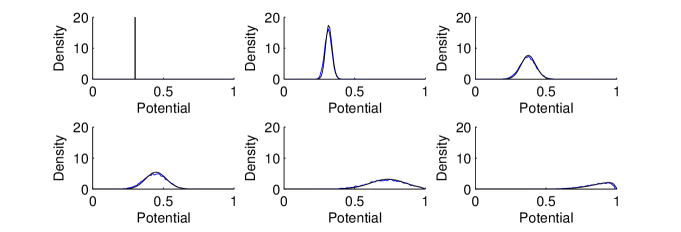
Figure 5: Simulation of the model (11) - (14), black curve, and the stochastic process (1), blue curve. A Dirac mass at the reset potential was taken as initial condition. The parameters of the simulation are $v_{r}=0.3$, $\mu=20$, $\sigma=0.4$. The plots show the evolution in time (age) of the solution at $a=0$, $a=0.1$, $a=0.3$, $a=0.5$, $a=0.7$, $a=7$.

$$\frac{\partial}{\partial a}q(a,v)+\overbrace{\frac{\partial}{\partial v}[(\mu-v)q(a,v)]}^{\text{Drift part}}-\overbrace{\frac{\sigma^{2}}{2}\frac{\partial^{2}}{\partial v^{2}}q(a,v)}^{\text{Diffusion}}=0,$$ (11)

again with an absorbing boundary condition for the threshold value $v=1$

$$q(a,1)=0,\forall a\geq 0,$$ (12)

and a reflecting boundary condition at the boundary $v=-\infty$

$$\lim\limits_{v\to-\infty}(-\mu+v)q(a,v)+\frac{\sigma^{2}}{2}\frac{\partial}{\partial v}q(a,v)=0,\forall a\geq 0.$$ (13)

Since a neuron firing an action potential is reset to $v_{r}$, we consider the initial density given by

$$q(0,v)=\delta(v-v_{r}),\quad v\in(-\infty,1),$$ (14)

where $\delta$ is the Dirac distribution. As for the equation (2), the equation (11) is often represented in terms of an integral equation. In this setting, the flux that we denote $\mathfrak{F}(a,v)$ is defined as

$$-\mathfrak{F}(a,v)=(-\mu+v)q(a,v)+\frac{\sigma^{2}}{2}\frac{\partial}{\partial v}q(a,v).$$

Therefore, the evolution in time of the density function $q$ is given by

$$\frac{\partial}{\partial a}q(a,v)=-\frac{\partial}{\partial v}\mathfrak{F}(a,v).$$

Note that, in the case considered here, the re-injection of the (probability) flux to the reset value (right hand side of equation (2)) is not considered, therefore the above model represents the evolution of the probability density of neurons before firing, i.e. in an inter-spike interval. The interpretation is that, once the neuron fired, it becomes of age zero, and the source term $\delta(v-v_{r})$ as initial condition can be understood intuitively as that, right after a spike the membrane potential is $v_{r}$ with probability $1$. It should be stressed that as the bias current $\mu$ and the noise intensity $\sigma$ do not depend on time, the probability density $q$ does not depend on time but only on age $a$. The flux at the threshold value, which is again given only by the diffusive part of the flux, is a measure of great interest since it gives the ISI distribution (for a neuron having at age $a=0$ the potential $v_{r}$):

$$ISI(a)=-\frac{\sigma^{2}}{2}\frac{\partial}{\partial v}q(a,1),\forall a\geq 0.$$ (15)

Until now, no analytical solution of the ISI curve has been found.

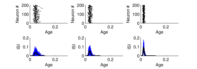
Figure 6: Simulation of the ISI function (15) via the FP formalism (11), black curve, respectively the stochastic process (1), blue curve. The parameters of the simulation are $v_{r}=0.3$, $\mu=15$ and $\sigma=0.4$ for the first simulation, $\mu=20$ and $\sigma=0.4$ for the second simulation and $\mu=30$, $\sigma=0.4$ for the third simulation. We also show the raster plot depicting the spike timing of $200$ neurons.

We present in Fig. 5 a simulation of the problem (11)–(14). Again, we have made a comparison between the stochastic process (blue curve) and the evolution in time of the density function (black curve). The simulation starts with a Dirac mass as initial condition (see first panel of Fig. 5). Under the influence of the drift term and the diffusion process (gaussian white noise), the density function spreads to the threshold. This is clearly seen in the upper plot of Fig. 5. At last, as expected, it converges to a zero density (see the last panel in Fig. 5). In Fig. 6, we make some different simulations of the ISI curve. As before, the blue curve corresponds to the stochastic process simulated via a Monte Carlo method, and the black curve - to the deterministic process (11). We present here three different panels corresponding to three different simulations where the bias current $\mu$ was increased. We also present a raster plot depicting the spike timing of each neuron simulated via the NLIF model (see upper panels of Fig 6). It can be clearly seen that, increasing the intensity current leads to a more concentrated ISI density. The ISI curve starts at zero, which means that right after spiking the neuron needs some time before spiking again. Then, the ISI curve increases and, after reaching a maximum, it decreases rapidly. This is depicted by the raster plot presented in Fig 6.

The first passage time problem is intimately related to the FP equation. Starting from the Chapman-Kolmogorov equation, it has been shown that the probability to find the state (potential) of a neuron at time $t$ in a certain value v, is the solution to the FP or Kolmogorov’s forward equation. From it, one can derive the equation that describes the evolution in time of the probability for a neuron that started at time $0$ from a potential value $v$ to not have reached yet the value threshold, named survival probability density. This equation is known as Kolmogorov’s backward equation, and the choice of boundary conditions has been discussed in Gardiner .

5 Noisy threshold model

In what follows, we shall use the concept of survival probability or survivor function as in gerstner . In our case, this function will be only age-dependent since we shall consider it for the case of a neuron that starts at age zero from the reset potential $v_{r}$.

Namely, if $q(a,v)$ is the solution to (11)-(14), then the following quantity

$$\int_{-\infty}^{1}q(a,v)\mbox{\rm\,d}v$$

stands for the probability of survival at age $a$ of a neuron that started at age $0$ from the position $v_{r}$. Again, ”survival” at age $a$ means that up to that time, the potential of the neuron’s membrane has not reached yet the threshold value. Then, the rate of decay of the survivor function

$$S(a)=-\dfrac{\frac{d}{da}\int_{-\infty}^{1}q(a,w)\,dw}{\int_{-\infty}^{1}q(a,w)\,dw}$$ (16)

represents the rate at which the threshold is reached and it has been called age-dependent death rate or hazard. $S(a)$ has the interpretation that, in order to emit a spike, the neuron has to ”survive” without firing in the interval $(0,a)$ and then fire at age $a$.

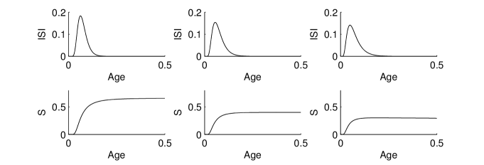
Figure 7: Simulation of the function $S(a)$ given by (16) in the lower panels and its corresponding $ISI$ given by (15) in the upper panels. The parameters of the simulation are $v_{r}=0.7$, $\mu=5$, $\sigma=0.1$, $\sigma=0.2$, $\sigma=0.3$.

In Fig. 7, numerical simulations of the age-dependent death rate for different parameters is presented. Let us notice that $S$ defines clearly a positive function that converges toward a constant. Indeed, $q(a,v)$ has the same asymptotic behavior as

$$e^{-\lambda a}q(v),$$

which implies that

$$\lim\limits_{a\to+\infty}S(a)=\lambda,$$

with $\lambda$ the dominant eigenvalue of the operator of the stationary FP equation and $q$ the corresponding eigenvector (see ost for example).

Note that $S$ can also be expressed in terms of the $ISI$ function given above

$$S(a)=-\dfrac{ISI(a)}{1-\int_{0}^{a}ISI(s)\,da}$$

which is the expression that we used in our numerical estimations of $S$.

We can now define properly the new stochastic process. The model is given by the evolution of the age of the neuron plus a stochastic reset mechanism to take into account the initiation of an action potential, and it is

$$\left\{\begin{array}[]{l}\displaystyle\frac{d}{dt}a(t)=1\\ \text{The spiking probability in $(t,t+dt)$ is given by $S(a(t))dt$}\\ \text{If a spike is triggered then $a(t)=0$},\end{array}\right.$$ (17)

where $S$ is the age-dependent death rate given by (16). In this model, the age of the neuron follows a trivial deterministic process, but the firing threshold is stochastic since at each time the neuron can fire. When this happens, its age is reset to zero. As reminded before, the difference between the models (1) and (17) is that, in the NLIF the dynamics are stochastic and the reset process is deterministic while in the escape-rate model above, the dynamics are deterministic but the reset mechanism is stochastic.

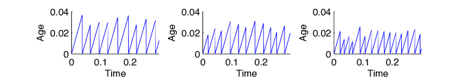
Figure 8: Simulation of the escape rate model (17). The parameters of the simulation are $v_{r}=0.7$, $\mu=5$, $\sigma=0.1$, $\sigma=0.2$, $\sigma=0.3$.

As we pointed out in the introduction, the escape-rate models have been introduced in plesser in order to arrive to more tractable models from mathematical point of view. It has been shown here that in the subthreshold regime for integrate and fire neurons, the diffusive noise can be replaced by a hazard noise (noisy threshold) described by a certain escape rate. More considerations about viable choices of age-dependent death rates as well as the derivation of the refractory-densities model that we will remind in the next section can be found in gerstner .

We present in Fig. 8 a numerical simulation of the stochastic process defined by (17) for different age-dependent death rates. Note that the neuron never fires exactly at the same age, since its probability to fire (escape) is purely stochastic.

6 The population density function (age-structure formalism)

We can now introduce the AS model in the same way as it has been done in gerstner , perthame03 and perthame04 .

The model describes the evolution in time of the population density function with respect to the age of a neuron in the following way: denoting by $n(t,a)$ the density of neurons at time $t$ at age $a$, then the evolution of $n$ is

$$\frac{\partial}{\partial t}n(t,a)+\overbrace{\frac{\partial}{\partial a}n(t,a)}^{\text{Drift part}}+\overbrace{S(a)n(t,a)}^{\text{Spiking term}}=0.\\$$ (18)

In Fig. 9, a schematic representation of the state space of the AS equation (18) is presented.

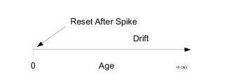
Figure 9: Schematic representation of the state space of the AS equation (18).

Because once a neuron triggers a spike, its age is reset to zero, we get the natural boundary condition

$$\overbrace{n(t,0)=r(t)}^{\text{Reset}},\quad\forall t>0,$$

where $r(t)$ is the firing rate and is given by

$$r(t)=\int_{0}^{+\infty}S(a)n(t,a)\,da,\quad\forall t\geq 0.$$ (19)

An initial distribution is assumed known:

$$n(0,a)=n_{0}(a),\quad\forall a>0.$$ (20)

In the above equations, $S(a)$ stands for the age-dependent death rate given by (16). Using the boundary condition and the expression of $r(t)$ given by (19), one can check easily the conservation property of the equation (2) by integrating it on the interval $(0,\infty)$, so that if the initial condition satisfies

$$\int_{0}^{+\infty}n_{0}(a)\,da=1,$$ (21)

the solution at any $t>0$ satisfies the normalization condition

$$\int_{0}^{+\infty}n(t,a)\,da=1.$$ (22)

We present in Fig. 10 a simulation of the problem (18)-(20). Again, we have made a comparison between the stochastic process (blue curve) given by (16) and the evolution in time of the density function (black curve) given by (18)-(20). The simulation starts with a Gaussian as initial condition (the first panel of Fig. 10). Under the influence of the drift term, the density function advances in age, which is clearly seen in the upper plots of Fig. 10. After the spiking process, the age of the neuron is reset to zero. The effect is well perceived in the lower panels of Fig. 10. As expected from the model, the density function converges to an equilibrium density (see the last panel in Fig. 10).

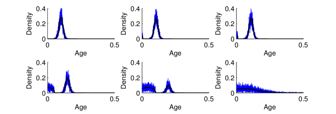
Figure 10: Simulation of the AS model (18)-(20). Inhere, the black curve represents the simulation of the AS model and the blue curve the simulation of the stochastic process (17). A gaussian was taken as initial condition; the parameters of the simulation are: $v_{r}=0.7$, $\mu=5$, $\sigma=0.1$. The six plots in the figure show the evolution in time of the solution at $t=0$, $t=0.1$, $t=0.3$, $t=0.5$, $t=0.7$, $t=7$.

The stationary state of the AS model can be easily computed; denoting by $r_{\infty}$ the stationary firing rate, we get:

$$n_{\infty}(a)=r_{\infty}e^{-\int_{0}^{a}S(s)\,ds},$$

and, if we take into account the normalization condition, we obtain the expression of the stationary firing rate

$$r_{\infty}^{-1}=\int_{0}^{+\infty}e^{-\int_{0}^{a}S(s)\,ds}\,da.$$

Since $\displaystyle e^{-\int_{0}^{a}S(s)\,ds}$ is the expression of the survivor function, its integral over $(0,\infty)$ has the interpretation of the mean firing time, therefore the last relation says nothing else than the fact that the stationary firing rate equals to the inverse of the mean firing time.

7 A theoretical link between the AS and FP problems

In this section, we present our main result that introduces an analytical link between the two formalisms, that states that there exists an integral transform that translates the solution to the problem (18)-(20) into the solution to (2)-(5).

Proposition 1

Let $p$ a solution to (2)-(5) and $n$ a solution to (18)-(20), and $p_{0}(v)$ and $n_{0}(a)$ two corresponding initial distributions. Then, if $p_{0}$ and $n_{0}$ satisfy

$$p_{0}(v)=\int_{0}^{+\infty}\frac{q(a,v)}{\int_{-\infty}^{1}q(a,w)\,dw}n_{0}(a)\,da,$$

the following relation holds true:

$$p(t,v)=\int_{0}^{+\infty}\frac{q(a,v)}{\int_{-\infty}^{1}q(a,w)\,dw}n(t,a)\,da.$$ (23)

Here, $q(a,v)$ is the solution to (11)-(14).

Remark 1

The integral transform given by the equation (23) can be interpreted with the help of probability theory. Since the integral $\int_{-\infty}^{1}q(a,w)\,dw$ is the survivor function and $q(a,v)$ is the probability density for a neuron to be at age $a$ and at potential $v$, the kernel of the transform can be interpreted as the probability density for a neuron to be at potential value $v$ given that it survived up to age $a$. The solution $n(t,a)$ denotes the density of population at time $t$ in state $a$, the integral over the whole possible states $a$ of the kernel multiplied by the density $n$ gives indeed the density of population at time $t$ in the state $v$.

Remark 2

In proposition 1, the integral transform is given in the sense of distributions, as we shall define it bellow.

Let us show for the beginning that the integral in (23) is well defined.
If we denote by $N(t,a)=\frac{n(t,a)}{\int_{-\infty}^{1}q(a,v)\mbox{\rm\,d}v}$, since

$$\frac{\partial}{\partial a}\frac{n(t,a)}{\int_{-\infty}^{1}q(a,v)\mbox{\rm\,d}v} = \frac{\frac{\partial}{\partial a}n(t,a)}{\int_{-\infty}^{1}q(a,v)\mbox{\rm\,d}v}+n(t,a)\left(\frac{\partial}{\partial a}\frac{1}{\int_{-\infty}^{1}q(a,v)\mbox{\rm\,d}v}\right)$$

$$= \frac{\frac{\partial}{\partial a}n(t,a)}{\int_{-\infty}^{1}q(a,v)\mbox{\rm\,d}v}+S(a)\frac{n(t,a)}{\int_{-\infty}^{1}q(a,v)\mbox{\rm\,d}v},$$

where we have used the definition of $S(a)$, one can see that $N$ is solution to the following system:

$$\left\{\begin{array}[]{ll}\frac{\partial}{\partial t}N(t,a)+\frac{\partial}{\partial a}N(t,a)=0,\\ N(t,0)=r(t)=\int_{0}^{\infty}ISI(a)N(t,a)\mbox{\rm\,d}a,\\ N(0,a)=\frac{n_{0}(a)}{{\int_{-\infty}^{1}q(a,v)\mbox{\rm\,d}v}}.\end{array}\right.$$ (24)

The system above can be easily integrated

$$N(t,a)=\left\{\begin{array}[]{ll}N_{0}(a-t),\quad a>t,\\ r(t-a),\quad t\geq a,\end{array}\right.$$

and the regularity of the solution is dictated by the regularity of the initial condition. In particular, if $N_{0}\in L^{1}(0,\infty)$ then $N(t,\cdot)\in L^{1}(0,\infty)$. Also, choosing $n_{0}$ such that $N_{0}\in H^{1}(0,\infty)$, and as soon as $N_{0}(0)=\displaystyle\int_{0}^{\infty}ISI(a)N_{0}(a)\mbox{\rm\,d}a$, we obtain that $N(t,\cdot)\in H^{1}(0,\infty)$.

On the other hand, $q(a,v)$ is the solution to (11)-(14), which is a parabolic equation with zero right hand side and homogeneous boundary conditions, therefore its exponential convergence towards zero as $a\rightarrow\infty$ for a.e. $v\in(-\infty,1]$ is immediate. We therefore can assert that, for every $\varepsilon$,

$$q(a,v)<c(v),\>\>a.e.\>\>v\in(-\infty,1],a>a_{\varepsilon}.$$

Since the product of a function from $L^{\infty}$ with an $L^{1}$ function is integrable, we have then that the transform (23) is well defined.

We also point out that, due to the large time behavior of $q$, we have that

$$\int_{0}^{\infty}S(a)\mbox{\rm\,d}a=+\infty,$$

condition which is known in age structured systems theory to imply that $n(t,a)$ tends to zero as $a$ tends to infinity (which can be easily seen by simply integrating (18) ). We have chosen to work on $[0,\infty)$ as the age interval, but one could have chosen, exactly as in AS systems theory, to work on a finite interval $[0,A_{\max}]$, where $A_{max}$ is the maximal age that can be reached. In this context, the condition that on the age interval, the integral of mortality rate to be infinity, has the biological interpretation that the density of the population at ages bigger than maximal one is zero, therefore the meaning of maximal age is exact. Of course, in our context, it would mean that all the neurons would have fired before reaching this maximal value. Also, let us notice that the system in $n$ has a classical solution on the defined domain; since the mortality rate does not depend explicitly on $t$, the derivatives with respect to $t$ and $a$ exist in classical sense.
Before starting the proof, let us make some considerations over the solutions to the systems (2)–(5), respectively (11)-(14). We shall consider weak solutions to both systems in the sense introduced in carillo01 , namely:

Definition 1

A pair of nonnegative functions $(p,r)$ such that

$$p\in L^{2}\left(0,T;L^{2}_{+}(-\infty,1)\right),r\in L^{2}_{+}(0,T)$$

is a solution to (2)–(5) if, for any test functions $\varphi(t,v)\in L^{2}([0,T]\times(-\infty,1])$ such that

$$\frac{\partial^{2}}{\partial v^{2}}\varphi(t,v),\frac{\partial}{\partial t}\varphi(t,v),(\mu-v)\frac{\partial}{\partial v}\varphi(t,v)\in L^{2}((0,T)\times(-\infty,1)),\varphi(T,v)=0,$$

the following relation takes place:

$$\int_{0}^{T}\int_{-\infty}^{1}p(t,v)\left[-\frac{\partial\varphi(t,v)}{\partial t}-(\mu-v)\frac{\partial\varphi(t,v)}{\partial v}-\frac{\sigma^{2}}{2}\frac{\partial^{2}\varphi(t,v)}{\partial v^{2}}\right]\mbox{\rm\,d}v\mbox{\rm\,d}t$$

$$=\int_{0}^{T}r(t)[\varphi(t,v_{r})-\varphi(t,1)]\mbox{\rm\,d}t+\int_{-\infty}^{1}p_{0}(v)\varphi(0,v)\mbox{\rm\,d}v.$$ (25)

As functions of the form $\Phi(v)\Psi(t)$ with $\Phi(v)\in L^{2}(-\infty,1)$ such that

$$(\mu-v)\Phi^{\prime}(v),\Phi^{\prime\prime}(v)\in L^{2}(-\infty,1),$$

and $\Psi(t)\in L^{2}(0,T)$ with $\Psi^{\prime}(t)\in L^{2}(0,T),\Psi(T)=0$ are a dense subset of the test functions in definition 1, we will restrict (1) to

$$\int_{0}^{T}\int_{-\infty}^{1}p(t,v)\left[-\Psi^{\prime}(t)\Phi(v)-\Psi(t)(\mu-v)\Phi^{\prime}(v)-\frac{\sigma^{2}}{2}\Psi(t)\Phi^{\prime\prime}(v)\right]\mbox{\rm\,d}v\mbox{\rm\,d}t=$$

$$\int_{0}^{T}r(t)[\Phi(v_{r})-\Phi(1)]\Psi(t)\mbox{\rm\,d}t+\int_{-\infty}^{1}p_{0}(v)\Phi(v)\Psi(0)\mbox{\rm\,d}v,$$ (26)

which gives the expression of the distributional derivative with respect to $t$:

$$\frac{\partial}{\partial t}\int_{-\infty}^{1}p(t,v)\Phi(v)\mbox{\rm\,d}v$$ (27)

$$=\int_{-\infty}^{1}p(t,v)\left[(\mu-v)\Phi^{\prime}(v)+\frac{\sigma^{2}}{2}\Phi^{\prime\prime}(v)\right]\mbox{\rm\,d}v+r(t)[\Phi(v_{r})-\Phi(1)],$$

again, for all the test functions $\Phi$ defined as above.

In the same way we will use a weak formulation for (11) as

$$\int_{0}^{\infty}\int_{-\infty}^{1}q(a,v)\left[-\chi^{\prime}(a)\Phi(v)-\chi(a)(\mu-v)\Phi^{\prime}(v)-\chi(a)\frac{\sigma^{2}}{2}\Phi^{\prime\prime}(v)\right]\mbox{\rm\,d}v\mbox{\rm\,d}a=$$

$$\Phi(v_{r})\chi(0)-\Phi(1)\int_{0}^{\infty}\chi(a)ISI(a)\mbox{\rm\,d}a,$$ (28)

with $\chi(a)\in L^{2}(0,\infty)$ and $\chi^{\prime}(a)\in L^{2}(0,\infty)$ and $\Phi(v)$ as in the previous definition.

We can now proceed with our proof.

Proof

Let us notice for the beginning that the AS system in $n(t,a)$ can be formulated equivalently as (24) in terms of the new variable

$$N(t,a)=\frac{n(t,a)}{\int_{-\infty}^{1}q(a,v)\mbox{\rm\,d}v}.$$

Moreover, using this notation, the integral transform reads:

$$p(t,v)=\int_{0}^{\infty}q(a,v)N(t,a)\mbox{\rm\,d}a.$$ (29)

In order to show that the above formula defines a solution to the FP system, let us apply the distributional derivative to (29) and show that it satisfies (27):

$$\frac{\partial}{\partial t}\int_{-\infty}^{1}p(t,v)\Phi(v)\mbox{\rm\,d}v=\int_{-\infty}^{1}\int_{0}^{\infty}q(a,v)\frac{\partial}{\partial t}N(t,a)\Phi(v)\mbox{\rm\,d}a\mbox{\rm\,d}v.$$

Using the fact that $N(t,a)$ is solution to (24), the last equation becomes:

$$\frac{\partial}{\partial t}\int_{-\infty}^{1}p(t,v)\Phi(v)\mbox{\rm\,d}v=-\int_{-\infty}^{1}\int_{0}^{\infty}q(a,v)\frac{\partial}{\partial a}N(t,a)\Phi(v)\mbox{\rm\,d}a\mbox{\rm\,d}v.$$

Let us turn now to the definition of the weak solution $q(a,v)$ given by (7). Noticing that, under proper assumptions over the initial state $N_{0}$, for each t arbitrary but fixed, $N(t,a)$ and $\frac{\partial}{\partial a}N(t,a)$ are in $L^{2}(0,\infty)$, we can apply the definition for $q$ by choosing $\chi(a)$ as $N(t,\cdot)$. Then we get that

$$-\int_{-\infty}^{1}\int_{0}^{\infty}q(a,v)\frac{\partial}{\partial a}N(t,a)\Phi(v)\mbox{\rm\,d}a\mbox{\rm\,d}v$$

$$=\int_{-\infty}^{1}\int_{0}^{\infty}N(t,a)q(a,v)\left[(\mu-v)\Phi^{\prime}(v)+\frac{\sigma^{2}}{2}\Phi^{\prime\prime}(v)\right]\mbox{\rm\,d}a\mbox{\rm\,d}v$$

$$+\Phi(v_{r})N(t,0)-\Phi(1)\int_{0}^{\infty}N(t,a)ISI(a)\mbox{\rm\,d}a.$$

Since $N(t,0)=r(t)=\displaystyle\int_{0}^{\infty}N(t,a)ISI(a)\mbox{\rm\,d}a$, the last two terms in the expression above give

$$r(t)[\Phi(v_{r})-\Phi(1)]$$

and therefore, we have obtained that

$$\frac{\partial}{\partial t}\int_{-\infty}^{1}\int_{0}^{\infty}q(a,v)N(t,a)\Phi(v)\mbox{\rm\,d}a\mbox{\rm\,d}v$$

$$=\int_{-\infty}^{1}\int_{0}^{\infty}q(a,v)N(t,a)\left[(\mu-v)\Phi^{\prime}(v)+\frac{\sigma^{2}}{2}\Phi^{\prime\prime}(v)\right]\mbox{\rm\,d}a\mbox{\rm\,d}v+r(t)[\Phi(v_{r})-\Phi(1)],$$

which is exactly (27) for $p(t,v)$ given by (29), which completes our proof.

The integral transform gives a corresponding relation between the two stationary states. Due to the form of the age-dependent death-rate $S$, the stationary density of the AS systems is completely determined by the solution to (11)-(14):

$$n_{\infty}(a)=\dfrac{\int_{-\infty}^{1}q(a,v)\,dv}{\int_{0}^{+\infty}\int_{-\infty}^{1}q(a,v)\,dv\,da}.$$

Using now the integral transform, we obtain that the stationary solution to (2)-(5) satisfies

$$p_{\infty}(v)=\dfrac{\int_{0}^{+\infty}q(a,v)\,da}{\int_{0}^{+\infty}\int_{-\infty}^{1}q(a,v)\,dv\,da}.$$

Since we have the relation

$$r_{\infty}=\frac{1}{\int_{0}^{+\infty}\int_{-\infty}^{1}q(a,v)\,dv\,da},$$

one may check directly that the above formula is indeed a solution to the stationary problem of the potential-structured system by multiplying (11) by $r_{\infty}$ and integrating it on $(0,\infty)$.

8 Asymptotic behavior

In the previous section, we have shown that there is an integral transform relating the solution of the time elapsed model and the solution of the FP equation. Our integral transform goes that way: for a density in age, $n(t,a)$, one can associate a corresponding solution $p(t,v)$ to the (2)-(5). Let us define the operator

$$\begin{array}[]{ccccc}F&:&L^{1}_{+}(0,+\infty)&\to&L^{1}_{+}(-\infty,1)\\ &&n_{\infty}&\mapsto&p_{\infty}\\ \end{array}$$

defined by

$$p_{\infty}(v)=\int_{0}^{+\infty}\frac{q(a,v)}{\int_{-\infty}^{1}q(a,w)\,dw}n_{\infty}(a)\,da,$$

where $p_{\infty}$ and $n_{\infty}$ are the stationary solutions to the potential- respectively age- structured systems. In the previous section, we have shown that, as soon as the initial conditions $p_{0}$ and $n_{0}$ are related by $F$, the whole trajectories $p(\cdot,v)$ and $n(\cdot,a)$ are also related by $F$. Here we show that in the case the relation between initial conditions is not satisfied, $F$ transforms the known convergence of $n$ to $n_{\infty}$ for $t\rightarrow\infty$ in the convergence of $p$ to $p_{\infty}=Fn_{\infty}$. This gives an additional way to study the behavior of $p$ for large time, already studied in carillo01 , carrillo02 by other means.

Proposition 2

For all initial conditions $p_{0}$ belonging to $L^{1}_{+}(-\infty,1)$, the solution $p$ of the potential structured problem (2)-(5) converges to $Fn_{\infty}$ where $n_{\infty}$ is such that, for any initial condition, the solution $n$ to (18), verifies

$$\lim\limits_{t\to+\infty}\|n(t,\cdot)-n_{\infty}(\cdot)\|_{L^{1}_{+}(0,\infty)}=0.$$

Proof

The model (18)-(20) is a classical McKendrick-von Foerster model, well known in population dynamics, with the particularity that the age specific mortality and fertility rates are the same. Then, defining the intrinsic reproduction number $\mathcal{R}_{0}$ as

$$\mathcal{R}_{0}=\int_{0}^{+\infty}S(a)\exp(-\int_{0}^{a}S(a^{\prime})da^{\prime})\mbox{\rm\,d}a,$$

by direct computations we get

$$\mathcal{R}_{0}=1.$$

Then it is well known that in this case, for $t\rightarrow\infty$, $n$ converges to $n_{\infty}$ satisfying

$$\frac{d}{da}n_{\infty}(a)+S(a)n_{\infty}(a)=0,\quad a>0,$$ (30)

with

$$n_{\infty}(0)=\int_{0}^{\infty}S(a)n_{\infty}(a)da,$$ (31)

and

$$\int_{0}^{\infty}n_{\infty}(a)da=1.$$ (32)

Let us now define $\alpha(t,v)$ the solution to:

$$\frac{\partial}{\partial t}\alpha(t,v)+\frac{\partial}{\partial v}[(\mu-v)\alpha(t,v)]-\frac{\sigma^{2}}{2}\frac{\partial^{2}}{\partial v^{2}}\alpha(t,v)=\delta(v-v_{r})r(t),$$

with boundary conditions similar to (3), (4), $r(t)$ being the firing rate relative to (18) and the initial condition is given by

$$\alpha(0,\cdot)=\alpha_{0}=Fn_{0}.$$

Then, thanks to Proposition 1,

$$\alpha(t,\cdot)=Fn(t,\cdot).$$

The transform $F$ being continuous from to $L^{1}_{+}(0,+\infty)$ to $L^{1}_{+}(-\infty,1)$, we get

$$\alpha(t,v)\rightarrow p_{\infty}(v)=Fn_{\infty}\mbox{ in }L^{1}(-\infty,1),$$

as $t\rightarrow\infty$, where one can check as in Proposition 1 that $p_{\infty}(v)$ satisfies

$$\begin{array}[]{ll}\frac{\partial}{\partial v}[(\mu-v)p_{\infty}(v)]-\frac{\sigma^{2}}{2}\frac{\partial^{2}}{\partial v^{2}}p_{\infty}(v)=\delta(v-v_{r})r_{\infty},\end{array}$$ (33)

with

$$r_{\infty}=-\frac{\sigma^{2}}{2}\frac{\partial}{\partial v}p_{\infty}(1),\\$$

and boundary conditions

$$\lim\limits_{v\to-\infty}(-\mu+v)p_{\infty}(v)+\frac{\sigma^{2}}{2}\frac{\partial}{\partial v}p_{\infty}(v)=0,\quad p_{\infty}(1)=0.$$

Now let us consider $\beta(t,v)=p(t,v)-\alpha(t,v)$. It satisfies

$$\frac{\partial}{\partial t}\beta(t,v)+\frac{\partial}{\partial v}[(\mu-v)\beta(t,v)]-\frac{\sigma^{2}}{2}\frac{\partial^{2}}{\partial v^{2}}\beta(t,v)=0,$$

with boundary conditions

$$\lim\limits_{v\to-\infty}(-\mu+v)\beta(t,v)+\frac{\sigma^{2}}{2}\frac{\partial}{\partial v}\beta(t,v)=0,\quad\beta(t,1)=0,$$

and with the initial condition given by:

$$\beta(0,v)=p_{0}(v)-Fn_{0}(a).$$

Using a change of variable similar to the one in carrillo02 , this equation is transformed in a heat equation on $(-\infty,0)$ with a zero Dirichlet condition in $0$. Then it is clear that $\beta(t,v)$ goes to $0$ as $t\rightarrow\infty$ in $L^{\infty}(-\infty,1)\cap L^{1}(-\infty,1)$, which ends the proof.

9 Conclusions and perspectives

It has been shown in plesser that the integrate-and-fire model with stochastic input can be mapped approximately onto an escape-rate model. Despite the fact that the two systems reproduce the same statistical activity, no analytical connection between them has been given until now. This paper is intended as a first step in this direction. We have proven here the existence of an exact analytical transform of the solution to the AS system into the solution to the F-P system which is an equivalent description of the NLIF model. Our finding highlights the theoretical relationships between the two stochastic processes and explain why the statistical firing distributions across time are similar for both models, see the red dots in Fig. 11. To our knowledge, such a result has not been proven until now.

As we have pointed it out in the introduction section, there are several advantages in using the AS formalism, and the main reason is that it has been already well-studied by mathematicians throughout the past decades. Another advantage in using the age structured model regards its numerical simulations, see Fig. 11. While the NLIF model requires the numerical implementation of the Euler-Maruyama scheme, the escape model can be simulated via a Gillespie-like algorithm. However, the noisy threshold model is probably a little bit more difficult to relate to the underlying biophysics of a cell. For this crucial point, one would prefer the use of NLIF model where each parameter of the model can be easily measured by neuroscientists.

We have to stress though that the results obtained here have been proven in the case of a not-connected neural population, which is a strong simplifying assumption. The case we considered is known in the framework of renewal systems as a stationary process. A possible extension of the present transform for the case of interconnected neurons remains thus for us an open issue to be investigated. But the most important thing to be investigated, and which is currently in working progress, is the existence of an inverse transform to the one introduced here. Nevertheless, in the absence of such an inverse transform, we proved here that the set of solutions to the F-P system defined through our transform is an attractor set of the solutions as $t$ tends to infinity.

The integral transform given in Proposition 1 has a probability meaning and this meaning can be interpreted using Bayes’ rule. Indeed, the kernel of our transformation can be read out as $\mathcal{P}(v|a)$, the probability to find a neuron at potential $v$ knowing its age $a$. The most important feature of this kernel is that it is time independent; the very nature of the age $a$ contains all the information about time that is needed to properly define the integral transform. On contrary, to define an inverse transform, one faces the problem of having a kernel that must depend on time. Transforming then the solution to the FP system into the solution to the AS system is therefore a little bit trickier. Another important aspect about the nature of the AS formalism is that the variable $a$ also entails information about the last firing moment. Indeed, attributing an age to a neuron presupposes that the considered neuron has already fired an action potential. From our perspective, the membrane potential variable $v$ does not carry out such knowledge. There is therefore a hidden information in the AS model that is not present in the FP approach. It is therefore our belief that, in order to properly define an inverse transform, one would be forced to assume that the FP initial density shares the information about the last firing event. A compatibility condition on the initial data is then required, we therefore believe that $p_{0}$ and $n_{0}$ should be related through the same transform presented in this paper.

The easiest way to formalize all this is probably to write down the Bayes’ rule

$$\mathcal{P}(a|v;t)=\mathcal{P}(v|a)*\mathcal{P}(a;t)/\mathcal{P}(v;t)=\mathcal{P}(v|a)*n(t,a)/p(t,v)$$

Note that the time-dependence of $\mathcal{P}(a|v;t)$ is inescapable. Moreover, the full form of $\mathcal{P}(a|v;t)$ is not useful within the context of an inverse transformation, since such an inverse transformation is trivial (reducing to $n(t,a)$ on both sides). Given these observations, it might make sense to assume that the system is close to equilibrium. With this maximum-entropy-like assumption, we can write a time-independent version of $\mathcal{P}(a|v;t)$:

$$\mathcal{P}(a|v)\approx\mathcal{P}(v|a)*n_{\infty}(a)/p_{\infty}(v)$$

where $n_{\infty}(a)$ and $p_{\infty}(v)$ are the equilibrium distributions for $n(t,a)$ and $p(t,v)$, respectively. These equilibriums can be calculated. With such reasoning, a perfect theoretical inverse from the AS model to the FP representations can be found, and an approximate inverse transformation can be constructed using the values of $n$ and $p$ at equilibrium, see Fig. 11.

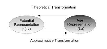
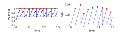
Figure 11: In the top panel, we show a schematic representation of the integral transformation between the two mathematical representations of the neural noise. In the bottom panel, we give two simulations illustrating the different mathematical treatments of noise in neuroscience context. The red dots indicates the firing time of the cell. The time distribution of those dots are similar in the two representations. The parameters of the simulation are $v_{r}=0.6$, $\mu=5$, $\sigma=0.2$.

As we stressed in the introduction, the benefit of such a representation would be the transfer of the analysis of special behaviors of the function $p(t,v)$ which is the solution of a system that raises technical problems, to the study of the behavior of the AS system, which is obviously simpler. The only quantity which will be significant then it will be the age dependent death rate which will contain all the information needed to give insights of the behavior of the system.

References

- (1) Abbott, L.: Lapique’s introduction of the integrate-and-fire model neuron (1907). Brain Research Bulletin 50(5), 303–304 (1999)
- (2) Abbott, L.F., van Vreeswijk, C.: Asynchronous states in networks of pulse-coupled oscillators. Phys. Rev. E. 48, 1483–1490 (1993)
- (3) Bressloff, P.C., Newby, J.M.: Stochastic models of intra-cellular transport. Review of Modern Physics 85 (1) (2013)
- (4) Brunel, N.: Dynamics of sparsely connected networks of excitatory and inhibitory spiking neurons. Journal of Computational Neuroscience 8, 183–208 (2000)
- (5) Brunel, N., Hakim, V.: Fast global oscillations in networks of integrate-and-fire neurons with low firing rates. Neural Computation 11, 1621–1671 (1999)
- (6) Brunel, N., van Rossum, M.: Lapicque’s 1907 paper: from frogs to integrate-and-fire. Biological Cybernetics 97, 341–349 (2007)
- (7) Burkitt, A.N.: A review of the integrate-and-fire neuron model: I. homogeneous synaptic input. Biological Cybernetics 95, 1–19 (2006)
- (8) Cáceres, M.J., Carrillo, J.A., Perthame, B.: Analysis of nonlinear noisy integrate & fire neuron models: blow-up and steady states. The Journal of Mathematical Neuroscience 1 (2011)
- (9) Carrillo, J.A., d M González, M., Gualdani, M.P., Schonbek, M.E.: Classical solutions for a nonlinear fokker-planck equation arising in computational neuroscience. Communications in PDEs 38, 385-409, 2013 38, 385–409 (2013)
- (10) Cox, D.R.: Renewal Theory. Mathuen, London (1962)
- (11) Dumont, G., Henry, J.: Population density models of integrate-and-fire neurons with jumps, well-posedness. Journal of Mathematical Biology 67(3), 453–81 (2013)
- (12) Dumont, G., Henry, J.: Synchronization of an excitatory integrate-and-fire neural network. Bulletin of Mathematical Biology 75(4), 629–48 (2013)
- (13) Dumont, G., Henry, J., Tarniceriu, C.: A density model for a population of theta neurons. Journal of Mathematical Neuroscience 4(1) (2014)
- (14) Ermentrout, G.B., Terman, D.: Mathematical foundations of neuroscience. Springer (2010)
- (15) Faisal, A., Selen, L., Wolpert, D.: Noise in the nervous system. Nature Reviews Neuroscience 9(4), 292–303 (2008)
- (16) Gardiner, C.W.: Handbook of Stochastic MMethod for Physics, Chemistry and Natural Sciences. Springer (1996)
- (17) Gerstner, W.: Time structure of the activity in neural network models. Phys. Rev. E. 51, 738–758 (1995)
- (18) Gerstner, W.: Population dynamics of spiking neurons: fast transients, asynchronous states, and locking. Neural Computation 12, 43–89 (2000)
- (19) Gerstner, W., Kistler, W.: Spiking neuron models. Cambridge university press (2002)
- (20) Gerstner, W., Naud, R.: How good are neuron models? Science 326(5951), 379–380 (2009)
- (21) Gillespie, D.T., Seitaridou, E.: Simple Brownian Diffusion: An Introduction to the Standard Theoretical Models. Oxford university press (2012)
- (22) Hodgkin, A.L., Huxley, A.F.: A quantitative description of membrane current and its application to conduction and excitation in nerve. The Journal of physiology 117(4), 500–544 (1952)
- (23) Holcman, D., Schuss, Z.: The narrow escape problem. SIAM Rev 56(2), 213–257 (2014)
- (24) Izhikevich, E.M.: Dynamical Systems in Neuroscience. The MIT Press (2007)
- (25) Knight, B.: Dynamics of encoding in neuron populations: Some general mathematical features. Neural Computation 12(3), 473–518 (2000)
- (26) Knight, B., Manin, D., Sirovich, L.: Dynamical models of interacting neuron populations in visual cortex. Robotics and cybernetics 54, 4–8 (1996)
- (27) Longtin, A.: Stochastic dynamical systems. Scholarpedia 5(4), 1619. (2010)
- (28) Longtin, A.: Neuronal noise. Scholarpedia 8(9), 1618 (2013)
- (29) Millman, D., Mihalas, S., Kirkwood, A., Niebur, E.: Self-organized criticality occurs in non-conservative neuronal networks during ‘up’ states. Nature physics 6, 801–805 (2010)
- (30) Newhall, K.A., Kovacic, G., Kramer, P.R., Cai, D.: Cascade-induced synchrony in stochastically-driven neuronal networks. Physical review 82 (2010)
- (31) Newhall, K.A., Kovacic, G., Kramer, P.R., Zhou, D., Rangan, A.V., Cai, D.: Dynamics of current-based, poisson driven, integrate-and-fire neuronal networks. Communications in Mathematical Sciences 8, 541–600 (2010)
- (32) Nykamp, D.Q., Tranchina, D.: A population density appraoch that facilitates large-scale modeling of neural networks : analysis and an application to orientation tuning. Journal of computational neurosciences 8, 19–50 (2000)
- (33) Omurtag, A., Knight, B., Sirovich, L.: On the simulation of large population of neurons. Journal of computational 8, 51–63 (2000)
- (34) Ostojic, S.: Interval interspike distributions of spiking neurons driven by fluctuating inputs. Journal of Neurophysiology 106, 361–373 (2011)
- (35) Ostojic, S., Brunel, N., Hakim, V.: Synchronization properties of networks of electrically coupled neurons in the presence of noise and heterogeneities. Journal of computational neurosciences 26, 369–392 (2009)
- (36) Pakdaman, K., Perthame, B., Salort, D.: Dynamics of a structured neuron population. Nonlinearity 23, 23–55 (2009)
- (37) Pakdaman, K., Perthame, B., Salort, D.: Relaxation and self-sustained oscillations in the time elapsed neuron network model. SIAM Journal of Applied Mathematics 73(3), 1260–1279 (2013)
- (38) Plesser, H.E., Gerstner, W.: Noise in integrate-and-fire neurons: from stochastic input to escape rates. Neural Computation 12(2), 367–384 (2000)
- (39) Schuss, Z., Singer, A., Holcman, D.: The narrow escape problem for diffusion in cellular domains. Proceedings of the National Academy of Sciences 104(41), 16,098 – 16,103 (2007)
- (40) Wilbur, W.J., Rinzel, J.: A theoretical basis for large coefficient of variation and bimodality in interspike interval distributions. J. Theor. Biol. 105, 345–368 (1983)