A Poroelastic Mixture Model of Mechanobiological Processes in Tissue Engineering.
Part II: Numerical Simulations

Abstract.

In Part I of this article we have developed a novel mechanobiological model of a Tissue Engineering process hat accounts for the mechanisms through which an isotropic or anisotropic adherence condition regulates the active functions of the cells in the construct. The model expresses mass balance and force equilibrium balance for a multi-phase mixture in a 3D computational domain and in time dependent conditions. In the present Part II, we study the mechanobiological model in a simplified 1D geometrical setting with the purpose of highlighting the ability of the formulation to represent the influence of force isotropy and nutrient availability on the growth of the tissue construct. In particular, an example of isotropy estimator is proposed and coded within a fixed-point solution map that is used at each discrete time level for system linearization and subsequent finite element approximation of the linearized equations. Extensively conducted simulations show that: 1) the spatial and temporal evolution of the cellular populations are in good agrement with the local growth/production conditions predicted by the mechanobiological stress-dependent model; and 2) the isotropy indicator and all model variables are strongly influenced by both maximum cell specific growth rate and mechanical boundary conditions enforced at the interface between the biomass construct and the interstitial fluid.

Keywords: Tissue Engineering; mechanobiology; numerical simulation.

Abbreviations: TE (tissue engineering); ECM (extracellular matrix); ACC (articular chondrocyte cell).

1. Introduction

In the mathematical model proposed and illustrated in Part I of the present research, the physical problem of tissue growth in a scaffold-based bioreactor is described by a system of PDEs constituted by: 1) the balance of mass for the solid and fluid phases of the growing mixture; 2) the continuity equation for the nutrient concentration; 3) the linear momentum balance equation for the mixture components.

In this second part we recast the mathematical picture in a simplified geometrical one-dimensional setting and we perform an accurate numerical simulation of the engineered construct with a twofold purpose. First, because of the complexity of the problem, we assess the reliability of model predictions by verifying that numerical results are biophysically reasonable and consistent with experimental measurements. Second, we single out the presence of some critical parameters in the mathematical formulation and investigate their role and quantitative influence on the evolution of mixture components.

An extensive set of numerical simulations, conducted to study the evolving construct under different working conditions, show that: 1) the computed cellular populations are in good agrement with the local growth/production conditions predicted by the mechanobiological stress-dependent model; and 2) the isotropy indicator, which in our model is responsible of the biological fate of the each cellular population, and consequently all the other model variables are strongly influenced by both maximum cell specific growth rate and mechanical boundary conditions enforced at the interface between the biomass construct and the interstitial fluid.

An outline of this Part II is as follows. In Sect. 2 we describe in detail the mechanobiological model in the one-dimensional spatial geometrical configuration. Sect. 3 is devoted to defining the stress indicator parameter $r$ and to providing a biophysical interpretation. In Sect. 4 we illustrate the computational algorithm that is used to solve the equation system of Sect. 2. Sections 5 and 6 contain the description and discussion of the various test cases numerically studied to validate the proposed model, while in Sect. 7 we address some future research perspectives.

2. The mechanobiological model in 1D

In this section we formulate the mechanobiological model proposed in Part I in a one-dimensional (1D) geometrical configuration (1D). In the remainder of the article we shortly write BVP and IV-BVP to denote ”boundary value problem” and ”initial value/boundary value problem”, respectively.

2.1. The one-dimensional computational domain

Fig. 1 (top panel) shows a (rather) simplified representation of the 3D scaffolded bioreactor used in the experimental analysis discussed in [13]. Denoting by $x$ the spatial coordinate, the region $x<0$ represents the scaffold wall, the open interval $\Omega=(0,L)$ is the growing tissue whereas the region $x>L$ corresponds to the interstitial fluid that brings nutrient to the growing construct. We denote by $\partial\Omega=\left\{0,\,L\right\}$ the boundary of the computational domain and by $n$ the outward unit normal vector on $\partial\Omega$. We have $n=-1$ at $x=0$ and $n=+1$ at $x=L$.

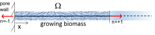
Figure 1. Top panel: schematic representation of a 1D scaffold-based bioreactor. Bottom panel: uniaxial stress state.

2.2. The one-dimensional model

The geometrical reduction introduced in the previous section implies that:

• all model variables depend on the sole spatial coordinate $x$ and on the time variable $t$;

• the solid displacement field $\mathbf{u}$ has only one nonvanishing component, that is $\mathbf{u}=[u,0,0]^{T}$ with $u=u(x,t)$;

• the strain tensor has only one nonvanishing component, that is

  $$\bm{\varepsilon}(\mathbf{u}(\mathbf{x},t))=\left[\begin{array}[]{ccc}\displaystyle\frac{\partial u(x,t)}{\partial x}&0&0\\[8.53581pt] 0&0&0\\ 0&0&0\end{array}\right].$$

The above analysis allows us to conclude that the simplified model of biomass growth considered in the present Part II can be regarded as a nonhomogeneous bar (fixed at one endpoint) subject to a uniaxial state of mechanical stress in such a way that each point $P=P(x,y,z)$ of every cross-section of the bar undergoes the same deformation ${\color[rgb]{0,0,0}\varepsilon_{xx}(\mathbf{u},t)}=\partial u(x,t)/\partial x$ (see Fig. 1, bottom panel).

2.2.1. Poroelastic IV-BVP for biomass

For given $\phi_{\eta}$ and $g_{\eta}$, $\eta=\textrm{cells},\textrm{ECM},\textrm{fl}$, find the solid displacement $u:\mathcal{Q}_{T_{end}}\rightarrow\mathbb{R}$ and the pressure $p:\mathcal{Q}_{T_{end}}\rightarrow\mathbb{R}$ that satisfy the following system of partial differential equations in balance form:

(1a) $$\displaystyle\frac{\partial T_{xx}}{\partial x}=0$$

(1b) $$\displaystyle\frac{\partial}{\partial t}\displaystyle\frac{\partial u}{\partial x}+\displaystyle\frac{\partial V}{\partial x}=0$$

(1c) $$V=-K(\phi_{\textrm{fl}})\frac{\partial p}{\partial x}$$

(1d) $$T_{xx}=H_{\mathrm{A}}\phi_{\textrm{s}}\displaystyle\frac{\partial u}{\partial x}-p-H_{\mathrm{A}}\phi_{\textrm{n}}g_{n}-H_{\mathrm{B}}\sum_{\eta=\textrm{v},\textrm{q},\textrm{ECM}}\phi_{\eta}g_{\eta}$$

where

(1e) $$K(\phi_{\textrm{fl}})=K_{\text{ref}}\Psi(\phi_{\textrm{fl}})$$

is tissue permeability with $$K_{\text{ref}}$$ defined in Eq. (10g) of Part I and

(1f) $$\Psi(\phi_{\textrm{fl}})=\displaystyle\frac{\phi_{\textrm{fl}}^{2}}{1-\phi_{\textrm{fl}}},$$

while $$H_{\mathrm{A}}=\lambda+2\mu H_{\mathrm{B}}=3\lambda+2\mu$$ is the so-called aggregate modulus [30] and . To close the problem, we specify the following initial and boundary conditions:

(1g) $$u(x,0)=u^{0}(x) \qquad\text{in}\quad\Omega$$

(1h) $$u(0,t)=0 \qquad\forall t\in(0,T)$$

(1i) $$T_{xx}(L,t)\cdot n=T_{\text{b}}(t) \qquad\forall t\in(0,T)$$

(1j) $$p(0,t)=0 \qquad\forall t\in(0,T)$$

(1k) $$V(L,t)\cdot n=V_{\text{b}}(t) \qquad\forall t\in(0,T).$$

For all times $t$, at $x=0$ we set an homogeneous Dirichlet boundary condition for the solid phase. This expresses the fact the solid phase is constrained at the scaffold wall. At $x=0$ we also enforce an homogeneous Neumann boundary condition for the fluid phase expressing hydraulic impermeability of the scaffold wall. At the interface with the interstitial fluid, $x=L$, we set a Neumann boundary condition for the solid phase. This expresses the fact that the fluid exerts a stress on the biomass. At $x=L$ we also enforce a Neumann boundary condition for the fluid phase by equating the Darcy flux to a given velocity of the external fluid.

2.2.2. Mass balance IV-BVP for nutrient concentration

For given $u$, $V$ and $\phi_{\eta}$, $\eta=\textrm{n},\textrm{v},\textrm{q},\textrm{fl}$, find the oxygen nutrient concentration $c:\mathcal{Q}_{T_{end}}\rightarrow\mathbb{R}^{+}$ that satisfies the following system of partial differential equations in balance form:

(2a) $$\frac{\partial c}{\partial t}+\frac{\partial J_{\mathrm{c}}}{\partial x}=Q_{\mathrm{c}}(\widetilde{\bm{\phi}},c)$$

(2b) $$J_{c}=v_{\textrm{fl}}c-D_{\mathrm{c}}\frac{\partial c}{\partial x}$$

where:

(2c) $$w=\frac{V}{\phi_{\textrm{fl}}}$$

(2d) $$v_{\textrm{fl}}=w+\dfrac{\partial u}{\partial t}$$

and

(2e) $$D_{\mathrm{c}}=D_{\mathrm{c},\textrm{fl}}\dfrac{3k-2\phi_{\textrm{fl}}(k-1)}{3+\phi_{\textrm{fl}}(k-1)},\qquad k:=K_{\mathrm{eq}}\dfrac{D_{\mathrm{c},\textrm{s}}}{D_{\mathrm{c},\textrm{fl}}}$$

(2f) $$Q_{\mathrm{c}}(\widetilde{\bm{\phi}},c)=-(R_{\textrm{n}}\phi_{\textrm{n}}+R_{\textrm{v}}\phi_{\textrm{v}}+R_{\textrm{q}}\phi_{\textrm{q}})\displaystyle\frac{c}{c+K_{1/2}}.$$

To close the problem, we specify the following initial and boundary conditions:

(2g) $$c(x,0)=c^{0}(x) \qquad\text{in }\Omega$$

(2h) $$\left.\dfrac{\partial c}{\partial x}\right|_{x=0}=0 \qquad\forall\,t$$

(2i) $$c(L,t)=c_{\text{ext}}(t).$$

As in the case of the cellular phase model, the Neumann boundary condition at $x=0$ represents the fact that the scaffold is impermeable to oxygen flow, while the Dirichlet boundary condition at $x=L$ indicates that we assume the interstitial fluid to deliver to the construct a prescribed amount of nutrient.

2.2.3. Mass conservation IV-BVP for cellular populations

For given $u$, $p$ and $c$, find the volume fractions $\widetilde{\bm{\phi}}=\left[\phi_{\textrm{n}},\,\phi_{\textrm{v}},\,\phi_{\textrm{q}},\,\phi_{\textrm{ECM}}\right]^{T}:(\mathcal{Q}_{T_{end}})^{4}\times(\mathbb{R}^{+})^{4}$ that satisfy the following system of partial differential equations in balance form:

(3a) $$\frac{\partial\widetilde{\bm{\phi}}}{\partial t}+\displaystyle\frac{\partial J_{\widetilde{\bm{\phi}}}}{\partial x}=\mathbf{Q}(\widetilde{\bm{\phi}},c,\mathbf{T})=(\mathbf{P}(\widetilde{\bm{\phi}},c,\mathbf{T})-\mathbf{C}(c,\mathbf{T}))\widetilde{\bm{\phi}}$$

(3b) $$\left(J_{\widetilde{\bm{\phi}}}\right)_{\eta}=\phi_{\eta}v_{\textrm{s}}-D_{\eta}\displaystyle\frac{\partial\phi_{\eta}}{\partial x} \eta=\textrm{cells},\textrm{ECM}$$

where $$v_{\textrm{s}}=\partial u/\partial t$$ is the solid phase velocity, the production terms are:

$$\mathbf{P}(\bm{\phi},c,\mathbf{T})=\Big{[}\phi_{\textrm{fl}}\dfrac{c}{K_{\text{sat}}+c}k_{\text{g}},\quad 0,\quad\beta_{\textrm{q}\textrm{n}}H_{r},\quad 0;$$

$$\qquad\qquad\qquad\qquad\;0,\qquad\;0,\quad\beta_{\textrm{q}\textrm{v}}\left(1-H_{r}\right),\quad 0;$$

$$\qquad\qquad\qquad\qquad\;\dfrac{1}{\tau_{\text{m}}},\quad\beta_{\textrm{v}\textrm{q}}H_{r},\quad 0,\quad 0;$$

(3c) $$\qquad\qquad\;0,\quad\dfrac{1}{V_{\textrm{cell}}}\,c\,E\,k_{\text{GAG}}\max\Big{[}0,1-\dfrac{\phi_{\text{ECM}}}{\phi_{\text{ECM,max}}}\Big{]},\quad 0,\quad 0\Big{]}$$

$$\mathbf{C}(c,\mathbf{T})=\mathrm{diag}\Big{(}\dfrac{1}{\tau_{\text{m}}}+k_{\textrm{qui}}(1-H_{c}),\;\beta_{\textrm{v}\textrm{q}}H_{r}+k_{\textrm{qui}}(1-H_{c})+k_{\text{apo}},$$

(3d) $$\qquad\quad\beta_{\textrm{q}\textrm{n}}H_{r}+\beta_{\textrm{q}\textrm{v}}\left(1-H_{r}\right)+k_{\textrm{qui}}\left(1-H_{c}\right)+k_{\text{apo}},\;k_{\text{deg}}\Big{)}.$$

and the fluid fraction is computed as

(3e) $$\phi_{\textrm{fl}}=1-\sum_{\eta=\textrm{n},\textrm{v},\textrm{q},\textrm{ECM}}\phi_{\eta}.$$

To close the problem, we specify the following initial and boundary conditions:

(3f) $$\widetilde{\bm{\phi}}(x,0)=\widetilde{\bm{\phi}}^{0}(x) \qquad\text{in }\Omega$$

(3g) $$\left.\dfrac{\partial\phi_{\eta}}{\partial x}\right|_{x=0}=0 \quad\qquad\forall\,t\qquad\eta=\textrm{n},\textrm{v},\textrm{q},\textrm{ECM}$$

(3h) $$\left.\dfrac{\partial\phi_{\eta}}{\partial x}\right|_{x=L}=0 \qquad\forall\,t\qquad\eta=\textrm{n},\textrm{v},\textrm{q},\textrm{ECM}.$$

The boundary conditions (3g)- (3h) express the fact that cellular phases can flow out of the biomass only because of the presence of an advective field.

3. Indicator of the isotropy of the local stress state

This section is devoted to the definition of the indicator $r$ of the isotropy of the local stress state. To this purpose, we observe that in the 1D configuration of Fig. 1, the total stress tensor $\mathbf{T}$ can be decomposed into the sum of isotropic and anisotropic components as

(4a) $$\mathbf{T}=\mathbf{T}_{\textrm{iso}}+\mathbf{T}_{\textrm{aniso}}$$

with:

(4b) $$\mathbf{T}_{\textrm{iso}}=\Big{[}\lambda\left(\phi_{\textrm{s}}\dfrac{\partial u}{\partial x}-g_{\textrm{n}}\phi_{\textrm{n}}\right)-\left(\dfrac{2}{3}\mu+\lambda\right)\sum_{\eta=\textrm{v},\textrm{q},\textrm{ECM}}g_{\eta}\phi_{\eta}-p\Big{]}\mathbf{I}$$

(4c) $$\mathbf{T}_{\textrm{aniso}}=2\mu\left(\phi_{\textrm{s}}\dfrac{\partial u}{\partial x}-g_{\textrm{n}}\phi_{\textrm{n}}\right)\mathbf{d}_{\textrm{pol}}\otimes\mathbf{d}_{\textrm{pol}},$$

and where $$\mathbf{d}_{\textrm{pol}} [1,0,0]^{T} \mathbf{T}_{\textrm{aniso}} x t r$$ is the unit vector . The decomposition (4a) suggests that can be used to measure the degree of anisotropicity of the stress state at any point of the mixture and at any time . With this aim, we define the parameter introduced in Section 5 of Part I as

(4d) $$r(x,t)=\displaystyle\frac{\|\mathbf{T}_{\textrm{aniso}}(x,t)\|_{F}}{2\mu}=\Big{|}\phi_{\textrm{s}}(x,t)\displaystyle\frac{\partial u(x,t)}{\partial x}-g_{\textrm{n}}(x,t)\phi_{\textrm{n}}(x,t)\Big{|}$$

where $$\|\mathbf{A}\|_{F} \mathbf{A}\in\mathbb{R}^{3\times 3} (x,t) \mathbf{T}$$ is the Frobenius norm of a matrix . We can give a mechanical interpretation of (4d) by studying the Mohr circle at point . The principal components of are:

(4e) $$\sigma_{\textrm{I}}=H_{\textrm{A}}\phi_{\textrm{s}}\dfrac{\partial u}{\partial x}-p-H_{\textrm{A}}g_{\textrm{n}}\phi_{\textrm{n}}-H_{\textrm{B}}\sum_{\eta=\textrm{v},\textrm{q},\textrm{ECM}}g_{\eta}\phi_{\eta}$$

(4f) $$\sigma_{\textrm{II}}=\sigma_{\textrm{III}}=\lambda\phi_{\textrm{s}}\dfrac{\partial u}{\partial x}-p-\lambda g_{\textrm{n}}\phi_{\textrm{n}}-H_{\textrm{B}}\sum_{\eta=\textrm{v},\textrm{q},\textrm{ECM}}g_{\eta}\phi_{\eta},$$

from which it follows that the Mohr circle at $$(x,t) C=\dfrac{\sigma_{\textrm{I}}+\sigma_{\textrm{II}}}{2} (x,t)$$ has center and radius equal to the maximum total shear stress at

$$\tau_{\textrm{max}}(x,t)=\dfrac{\sigma_{\textrm{I}}(x,t)-\sigma_{\textrm{II}}(x,t)}{2}=\mu\left(\phi_{\textrm{s}}(x,t)\displaystyle\frac{\partial u(x,t)}{\partial x}-g_{\textrm{n}}(x,t)\phi_{\textrm{n}}(x,t)\right).$$

Comparing this latter relation with (4d) we conclude that the indicator of the local stress state anisotropy can be written as

(4g) $$r(x,t)=\displaystyle\frac{|\tau_{\textrm{max}}(x,t)|}{\mu}.$$

According to Eq. (7a) of Part I, we need also characterize an appropriate value for the threshold parameter $$\bar{r}$$ representing the level of hydrodynamic shear stress that induces metabolic activity of the cell population n and therefore separates the isotropic regime from the anisotropic regime. In [23, 24] it is shown that hydrodynamic shear below 10 mPa may promote GAG synthesis, so that, coherently with (4g), we assume

(4h) $$\bar{r}=\dfrac{\mathrm{10mPa}}{\mu}.$$

4. Numerical approximation of the 1D mechanobiological model

In this section we focus on the numerical approximation of the model illustrated in Sect. 2. With this purpose, we illustrate in Sect. 4.1 the computational algorithm to iteratively solve the coupled systems of equations and in Sect. 4.2 we shortly discuss the finite element discretization scheme used to numerically solve the linearized equations.

4.1. Computational algorithm

Solving in closed form the mechanobiological model illustrated in Sect. 2.2 is a very difficult task because of the strong nonlinear nature of the problem. Therefore, a numerical treatment is in order. Prior to discretization we need to reduce the solution of the whole coupled system to the solution of a sequence of linearized equations of simpler form. For this purpose we set

(5a) $$\mathbf{U}=\left[u,p,\phi_{\textrm{n}},\phi_{\textrm{v}},\phi_{\textrm{q}},\phi_{\textrm{ECM}},c\right]^{T}$$

and subdivide the time interval $$[0,T_{end}] N_{T}\geq 1 \Delta t=T_{end}/N_{T} t^{n}=n\Delta t n=0,\ldots,N_{T} n=0,\ldots,N_{T}-1$$ into uniform subintervals of length , in such a way that the discrete time levels , , are obtained. Then, for each , we set

$$\mathbf{U}^{(0)}:=\mathbf{U}^{n},$$

and for all $$m\geq 0$$ until convergence we perform the following fixed point iteration:

1. solve the linear poroelastic system:

   (5b) $$\displaystyle\frac{\partial T_{xx}^{(m+1)}}{\partial x}=0$$

   (5c) $$\displaystyle\frac{1}{\Delta t}\displaystyle\frac{\partial u^{(m+1)}}{\partial x}+\displaystyle\frac{\partial V^{(m+1)}}{\partial x}=\displaystyle\frac{1}{\Delta t}\displaystyle\frac{\partial u^{n}}{\partial x}$$

   (5d) $$V^{(m+1)}=-K(\phi_{\textrm{fl}}^{(m)})\frac{\partial p^{(m+1)}}{\partial x}$$

   (5e) $$T_{xx}^{(m+1)}=H_{\mathrm{A}}\phi_{\textrm{s}}^{(m)}\displaystyle\frac{\partial u^{(m+1)}}{\partial x}-p^{(m+1)}-H_{\mathrm{A}}\phi_{\textrm{n}}^{(m)}g_{n}^{(m)}-H_{\mathrm{B}}\sum_{\eta=\textrm{v},\textrm{q},\textrm{ECM}}\phi_{\eta}^{(m)}g_{\eta}^{(m)}$$

   supplied by the boundary conditions (1h)- (1k). This yields the updated solid displacement $u^{(m+1)}$ and fluid pressure $p^{(m+1)}$;

2. solve the linear advection-diffusion-reaction (ADR) system:

   (5f) $$\frac{c^{(m+1)}}{\Delta t}+\frac{\partial J_{\mathrm{c}}^{(m+1)}}{\partial x}-\widehat{Q}_{\mathrm{c}}^{(m)}(\widetilde{\bm{\phi}}^{(m)},c^{(m)})c^{(m+1)}=\frac{c^{n}}{\Delta t}$$

   (5g) $$J_{c}^{(m+1)}=v_{\textrm{fl}}^{(m+1)}c^{(m+1)}-D_{\mathrm{c}}^{(m)}\frac{\partial c^{(m+1)}}{\partial x}$$

   where:

   (5h) $$w^{(m+1)}=\frac{V^{(m+1)}}{\phi_{\textrm{fl}}^{(m)}}$$

   (5i) $$v_{\textrm{fl}}^{(m+1)}=w^{(m+1)}+\dfrac{u^{(m+1)}-u^{n}}{\Delta t}$$

   and

   (5j) $$D_{\mathrm{c}}^{(m)}=D_{\mathrm{c},\textrm{fl}}\dfrac{3k-2\phi_{\textrm{fl}}^{(m)}(k-1)}{3+\phi_{\textrm{fl}}^{(m)}(k-1)},\qquad k:=K_{\mathrm{eq}}\dfrac{D_{\mathrm{c},\textrm{s}}}{D_{\mathrm{c},\textrm{fl}}}$$

   (5k) $$\widehat{Q}_{\mathrm{c}}^{(m)}(\widetilde{\bm{\phi}}^{(m)},c^{(m)})=-(R_{\textrm{n}}\phi_{\textrm{n}}^{(m)}+R_{\textrm{v}}\phi_{\textrm{v}}^{(m)}+R_{\textrm{q}}\phi_{\textrm{q}}^{(m)})\displaystyle\frac{1}{c^{(m)}+K_{1/2}}$$

   supplied by the boundary conditions (2h)- (2i). This yields the updated oxygen concentration $c^{(m+1)}$;

3. solve the linear advection-diffusion-reaction system:

   $$\frac{\widetilde{\bm{\phi}}^{(m+1)}}{\Delta t}+\displaystyle\frac{\partial J_{\widetilde{\bm{\phi}}}^{(m+1)}}{\partial x}+\mathbf{C}(c^{(m+1)},\mathbf{T}^{(m+1)}))\widetilde{\bm{\phi}}^{(m+1)}=$$

   (5l) $$\mathbf{P}(\widetilde{\bm{\phi}}^{(m)},c^{(m+1)},\mathbf{T}^{(m+1)})\widetilde{\bm{\phi}}^{(m)}$$

   (5m) $$\left(J_{\widetilde{\bm{\phi}}}\right)_{\eta}^{(m+1)}=\phi_{\eta}^{(m+1)}v_{\textrm{s}}^{(m+1)}-D_{\eta}\displaystyle\frac{\partial\phi_{\eta}^{(m+1)}}{\partial x}\qquad\eta=\textrm{cells},\textrm{ECM}$$

   supplied by the boundary conditions (3g)- (3h). This yields the updated cellular volume fractions $\bm{\phi}^{(m+1)}$.

Should the above fixed point iteration 1.-3. reach convergence at a certain value $m^{\ast}\geq 0$, then we set

$$\mathbf{U}^{n+1}:=\mathbf{U}^{(m^{\ast})}$$

and we increment the time loop counter by setting

$$n\leftarrow n+1.$$

until conclusion of the time advancement loop.

Two remarks are in order about the above described solution map. The first remark concerns with the linear poroelastic system (5b)- (5e). The weak formulation of this problem leads to solving a saddle-point problem in block symmetric form to which the abstract analysis of [19], Chapt. 7 and [2] can be applied to prove existence and uniqueness of the solution pair $u^{(m+1)},\,p^{(m+1)}$. The second remark concerns with the two linear ADR problems. The splitting of the source term ${Q}_{\mathrm{c}}$ in (2a) and $\mathbf{Q}$ in (3a) gives rise to two BVPs to which the application of the maximum principle (see [25]) allows to prove nonnegativity of the solutions $c^{(m+1)}$ and $\phi_{\eta}^{(m+1)}$, $\eta=\textrm{cells},\textrm{ECM}$.

4.2. Finite element discretization

The computational procedure described in Sect. 4.1 leads to solving two kinds of BVPs: (i) a saddle-point problem; (ii) two ADR equations. We numerically solve (i) and (ii) using the Galerkin finite element approximation scheme on a family of partitions $\left\{\mathcal{T}_{h}\right\}_{h>0}$ of the computational domain, $h$ being the discretization parameter (see [19]). In the case of the saddle point problem (i) we employ piecewise linear finite elements on $\mathcal{T}_{h}$ for both solid displacement and fluid pressure. Equal-order interpolation for $u$ and $p$ does not give rise to numerical instabilities as it would be the case if the Stokes equations for an incompressible fluid were to be solved (cf. [19], Chapt. 9), because in the present model the variable $p$ is not a Lagrange multiplier (as in the Stokes system), rather, it is the solution of the elliptic Darcy problem (1b)-(1c). In the case of the ADR equation we employ for the approximation of the concentration and of the cellular volume fractions the primal-mixed finite element discretization scheme with exponential fitting stabilization proposed and investigated in [26]. This choice is taken because it ensures that the computed numerical solutions satisfy a strict positivity property even in the case of a strongly advective regime. Moreover, it can be checked that, if advective terms do not play a major role compared to oxygen molecular diffusion in the biomass, then the effect of the stabilization introduced by the primal-mixed method of [26] becomes negligible so that the accuracy of the scheme is not spoiled. This, instead, would not be the case if the classic upwind stabilization were adopted (see [3] for a discussion of this important issue).

5. Simulation tests

In this section we show the numerical results obtained by solving the 1D problem with the computational algorithm described in Sect. 4. Two sets of simulation tests are performed. In the first set of simulations we set $T_{\text{b}}=V_{\text{b}}=0$ in Eqns. (1i)-(1k). This corresponds to investigating a static culture environment (see [23, 24]). In the second set of simulations we set $T_{\text{b}}=100\mathrm{mPa}$ and $V_{\text{b}}=50\mathrm{\mu ms^{-1}}$ as in [5]. These values are characteristic of a culture in a perfusion bioreactor where an external hydrodynamic shear stress is applied [27, 21, 24].

The principal scope of the numerical experiments is to perform a sensitivity analysis of the model and its effect on the predicted profiles of cellular components. This analysis allows a biophysical validation of the proposed model and may provide a useful guideline for an optimal design and calibration of a bioreactor in TE applications.

The first investigated input model parameter is the amount $A$ of cell density at the beginning of the culture process ($t=0$) and at the pore wall ($x=0$). We adopt the following exponentially decaying profiles for cells and ECM at $t=0$:

(6a) $$\phi_{\textrm{n}} =A_{\textrm{n}}\exp(-x/L_{d})$$

(6b) $$\phi_{\eta} =A_{\eta}\exp(-x/L_{d})\qquad\eta=\textrm{v},\textrm{q},\textrm{ECM},$$

with $$L_{d}=L/5 A$$, and for each set of simulations we use the following values of :

The above values of $$A_{n} A_{\eta}$$ and agree with the biophysical evidence that at the beginning of the growth process, proliferating cells are present in larger amount than the other cellular populations.

The second investigated input model parameter is the cellular growth rate $k_{\text{g}}$. In our computations we use two values of this parameter, $k_{\text{g1}}$ and $k_{\text{g2}}$ (cf. Tab. 1). These two values are selected by comparison with the maximum specific cell growth rate $k_{\text{g0}}$ used in [27] in such a way that $k_{\text{g}}<k_{\text{g0}}$ corresponds to ”low growth regime” whereas $k_{\text{g}}>k_{\text{g0}}$ corresponds to ”high growth regime”.

The third investigated input model parameter is the maximum value of the external oxygen concentration $c_{\text{ext}}$ in Eq. (2h) that is supplied to the growing structure by the surrounding environment. To determine the effect of oxygen availability on biomass growth we set $c_{\text{ext}}(t)=c_{\text{sat}}$ and $c_{\text{ext}}(t)=c_{\text{thr}}$ for all $t\in[0,T_{end}]$, $c_{\text{sat}}$ and $c_{\text{thr}}$ being the saturation and threshold oxygen concentration, respectively (see Sect. 5 of Part I and Tab. 1).

We conclude this introduction to numerical simulations by defining the following new (equivalent) parameter $\xi=\xi(r)$ for a synthetic representation of the isotropy indicator $r$

(6c) $$\xi(r):=\begin{cases}1&\quad\text{if}\,r<\bar{r}\\ 0&\quad\text{if}\,r>\bar{r}.\end{cases}$$

In the remainder of the discussion, no plot is reported for the fluid volume fraction $\phi_{\textrm{fl}}$ because this variable can be computed by post-processing using (3e). Simulations are run over the time interval $[0,T_{end}]$, with $T_{end}=30$ days, and the one-dimensional plots show the time evolution of the solid and fluid mixture components at the spatial coordinate $x=L/2$. The values of model parameters used in the numerical experiments are reported in Tab. 1.

5.1. Static culture

In this section the boundary data of the poroelastic system  (1) are $V_{b}=T_{b}=0$ while the external nutrient concentration $c_{\rm ext}$ is equal to $c_{\rm sat}$ and $c_{\rm thr}$, respectively.

5.1.1. Initial condition IC1

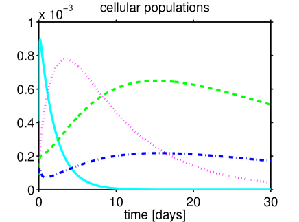
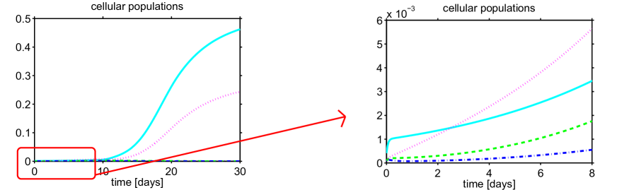
Figure 2. Temporal evolution of cellular populations and ECM in the static culture for $c_{\text{ext}}=c_{\text{sat}}$. Initial condition IC1. Top: $k_{\text{g}}=k_{\text{g1}}$. Bottom left: $k_{\text{g}}=k_{\text{g2}}$. Bottom right: $k_{\text{g}}=k_{\text{g2}}$, zoom of the first eight days of culture. Solid line: $\phi_{\textrm{n}}$; dashed line: $\phi_{\textrm{v}}$; dotted line: $\phi_{\textrm{q}}$; dash-dot line: $\phi_{\textrm{ECM}}$.

Figure 2 illustrates the comparison between the behavior of cell populations and ECM for two different values of the cell growth rate and in correspondence of a very high level of nutrient concentration ($c_{\text{ext}}=c_{\text{sat}}$). In the low growth regime ($k_{\text{g}}=k_{\text{g,1}}$), cell mitosis experiences a drastic increase during the first days of culture, then the volumetric fraction of proliferating cells diminishes and rapidly tends to zero (Fig. 2, top panel). On the other hand synthesizing cells slowly increase and reach the maximum value after about 10 days of culture. Due to cell apoptosis and ECM degradation, all the solid volumetric fractions tend to vanish as culture time increases. This behavior is in accordance with the situation described by the experimental set-up, where, during the first days of culture, cells proliferate intensively, and then after 10-12 days, the cell-polymer construct starts to increase in size mainly due to ECM deposition [18, 17]. The above described scenario is also consistent with the behavior of the parameter $\xi$ that predicts an isotropic adherence state at each time $t>0$ and at each point $x$ of the growing biomass (Fig. 3, left panel).

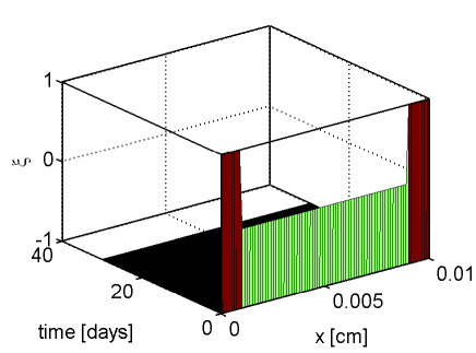
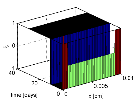
Figure 3. Spatial and temporal evolution of parameter $\xi$ in the static culture for $c_{\text{ext}}=c_{\text{sat}}$. Initial condition IC1. Left: $k_{\text{g}}=k_{\text{g1}}$. Right: $k_{\text{g}}=k_{\text{g2}}$.

In the high growth regime ($k_{\text{g}}=k_{\text{g,2}}$) the mitotic profile apparently evolves in a complimentary way with respect to the low growth case (Fig. 2, bottom left panel). The $\textrm{n}-$cell density markedly increases after 10 days of culture, whereas the evolution of the ECM density is negligible. Actually, Fig. 2, bottom right panel, shows that, in the very initial phase of the cultivation, the growth of proliferating cells is similar to that in the low growth situation. However, once the corresponding maximum in the low growth regime has been reached, mitotic activity persists because of the up-regulated growth rate and, after about 30 days of culture, stabilizes around a point of equilibrium. Note that in Fig. 2, bottom left panel, the increase of $\phi_{\textrm{n}}$ becomes significant in correspondence of the manifestation of the anisotropic region in Fig. 3 (right panel).

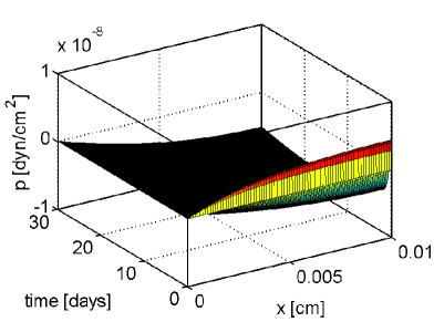
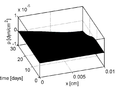
Figure 4. Spatial and temporal evolution of fluid pressure in the static culture for $c_{\text{ext}}=c_{\text{sat}}$. Initial condition IC1. Left: $k_{\text{g}}=k_{\text{g1}}$. Right: $k_{\text{g}}=k_{\text{g2}}$.

The spatial and temporal distribution of fluid pressure is shown in Fig. 4. We notice that the fluid pressure drop is significantly larger in the high growth regime (right panel) than in the lower growth regime (left panel). This different quantitative response of the fluid phase agrees with the above predicted cellular populations and expresses the biophysical fact that the larger the cellular phase, the larger the forces exerted by this latter on the fluid. We also notice that the spatial distribution in the low growth regime is remarkably different from that in the high growth regime. In the former case (left panel) the simulated working conditions practically correspond to a linear Darcy hydraulic model with constant permeability, subject to mixed homogeneous boundary conditions and to a constant strain rate spatial distribution from which it follows that the fluid pressure attains a parabolic profile. In the latter case (right panel) the simulated working conditions significantly deviate from a linear Darcy hydraulic model because of the increase of cellular populations around the time level $t=12$ days which corresponds to a decrease of the hydraulic permeability of the mixture in accordance with (1f) and, consequently, to an increase of the pressure drop compared to the low growth condition.

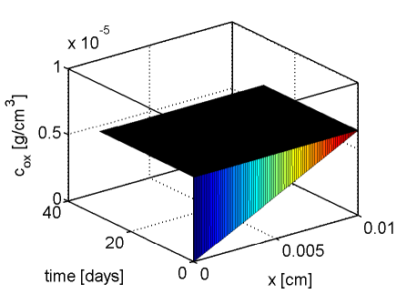
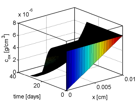
Figure 5. Spatial and temporal evolution of oxygen concentration in the static culture for $c_{\text{ext}}=c_{\text{sat}}$. Initial condition IC1. Left: $k_{\text{g}}=k_{\text{g1}}$. Right: $k_{\text{g}}=k_{\text{g2}}$.

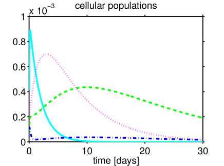
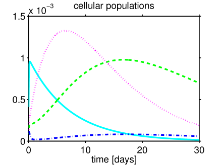
Figure 6. Temporal evolution of cellular populations and ECM in the static culture for $c_{\text{ext}}=c_{\text{thr}}$. Initial condition IC1. Left: $k_{\text{g}}=k_{\text{g1}}$. Right: $k_{\text{g}}=k_{\text{g2}}$. Solid line: $\phi_{\textrm{n}}$; dashed line: $\phi_{\textrm{v}}$; dotted line: $\phi_{\textrm{q}}$; dash-dot line: $\phi_{\textrm{ECM}}$.

The spatial and temporal distribution of delivered nutrient concentration is shown in Fig. 5. In the low growth regime (left panel) oxygen consumption is practically equal to zero whereas in the high growth regime (right panel) it becomes clearly visible in correspondence of the onset of the anisotropic stress state (Fig. 3, right panel) and of the drastic increase of proliferating cells (Fig. 2, bottom left). The marked nonuniformity in the spatial distribution of oxygen in Fig. 5, right panel, is to be ascribed to the rather different boundary conditions at $x=0$ (null diffusive flux) and at $x=L$ (nutrient concentration in local equilibrium with the externally supplied value).

Fig. 6 shows the time evolution of cell populations and ECM in correspondence of a reduced (but still high) level of nutrient concentration ($c_{\text{ext}}=c_{\text{thr}}$). In the low growth regime the evolution of cell populations is very similar to the case where $c_{\text{ext}}=c_{\text{sat}}$ (Fig. 6, left) while the ECM concentration undergoes a clear decrease due to the fact that the supply of growth factors is not sufficient to promote both cell mitosis and biosynthesis. In the high growth regime the n-cell profile is very similar to the profile in the low growth regime, except for a delayed decrease, while synthesizing cells exhibit a markedly visible increase (Fig. 6, right panel), reaching approximately the same maximum value as that of proliferating cells. This interesting biophysical result may be ascribed to the increased growth rate $k_{\text{g2}}$ that promotes mitotic activity at the expense of a very low oxygen consumption. As a consequence, the nutrient contained in the fluid is made completely available for secreting cells that increase their density within the growing tissue and, accordingly, their biomass production.

5.1.2. Initial condition IC2

In this second set of simulations, the initial seeding density of cells increase by an order of magnitude with respect to the initial density in condition IC1.

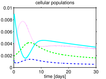
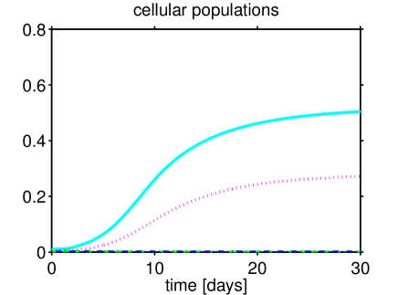
Figure 7. Temporal evolution of cellular populations and ECM in the static culture for $c_{\text{ext}}=c_{\text{sat}}$. Initial condition IC2. Left: $k_{\text{g}}=k_{\text{g1}}$. Right: $k_{\text{g}}=k_{\text{g2}}$. Solid line: $\phi_{\textrm{n}}$; dashed line: $\phi_{\textrm{v}}$; dotted line: $\phi_{\textrm{q}}$; dash-dot line: $\phi_{\textrm{ECM}}$.

The resulting response of the system in the low growth regime displays an oscillatory evolution of the solid volumetric fractions before approaching the equilibrium stable state $(\phi_{\textrm{n}},\phi_{\textrm{v}},\phi_{\textrm{q}},\phi_{\textrm{ECM}})=(0,0,0,0)^{T}$. In particular, as shown in Fig. 7, left panel, proliferating cells, in addition to the initial spike already visible in the case IC1, exhibit a second (smaller) growth peak at about 10 days of culture, and then start again to slowly decrease. This fluctuation may be interpreted as an oscillation around a mean value, that represents the average level of proliferation measured in the first two weeks of the experiments. As a matter of fact, as shown in [11], at high seeding density no significant change in cell number was measured after 2 weeks of culture (see Fig. 3c of [11]). Model predictions suggest that high initial seeding densities might negatively affect biomass growth, because, on the one hand, increased cell-cell contact might inhibit the formation of new colonies, and, on the other hand, because nutrient availability, although being abundant at the beginning of the culture process, becomes insufficient so that cellular metabolism looses its functionality.

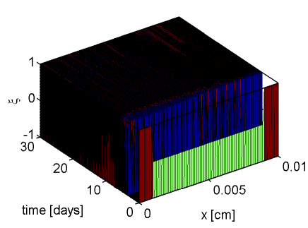
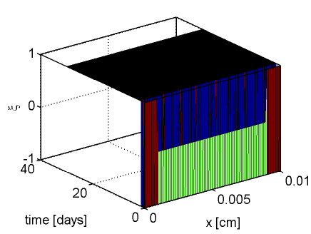
Figure 8. Spatial and temporal evolution of parameter $\xi$ in the static culture for $c_{\text{ext}}=c_{\text{thr}}$. Initial condition IC2. Left: $k_{\text{g}}=k_{\text{g1}}$. Right: $k_{\text{g}}=k_{\text{g2}}$.

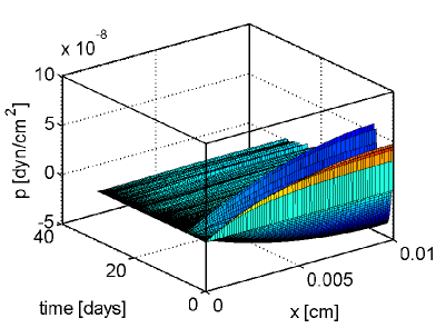
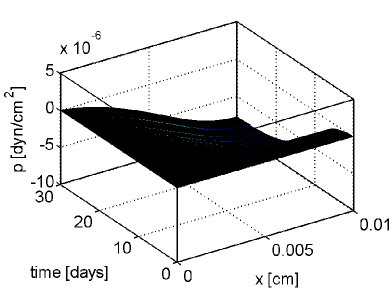
Figure 9. Spatial and temporal evolution of fluid pressure in the static culture for $c_{\text{ext}}=c_{\text{sat}}$. Initial condition IC2. Left: $k_{\text{g}}=k_{\text{g1}}$. Right: $k_{\text{g}}=k_{\text{g2}}$.

The oscillatory behavior of proliferating cells shown in Fig. 7 left is manifested also in the time evolution of $\xi$ (Fig. 8, left panel) and $p$ (Fig. 9, left panel). The mechanical stress in the biomass oscillates around the isotropic state while the fluid pressure oscillates around a constant value, and these fluctuations persist until the end of the simulation.

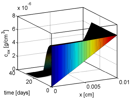
Figure 10. Spatial and temporal evolution of oxygen concentration in the static culture for $c_{\text{ext}}=c_{\text{sat}}$. Initial condition IC2. Left: $k_{\text{g}}=k_{\text{g1}}$. Right: $k_{\text{g}}=k_{\text{g2}}$.

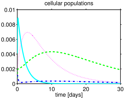
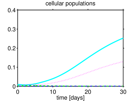
Figure 11. Temporal evolution of cellular populations and ECM in the static culture for $c_{\text{ext}}=c_{\text{thr}}$. Initial condition IC2. Left: $k_{\text{g}}=k_{\text{g1}}$. Right: $k_{\text{g}}=k_{\text{g2}}$. Solid line: $\phi_{\textrm{n}}$; dashed line: $\phi_{\textrm{v}}$; dotted line: $\phi_{\textrm{q}}$; dash-dot line: $\phi_{\textrm{ECM}}$.

In the high growth regime, the behavior of cells and ECM (Fig. 7, right panel) is very similar to that of Sect. 5.1.1 (cf. Fig. 2, left bottom panel). We notice that the switch from isotropic to anisotropic stress conditions predicted by parameter $\xi$ (Fig. 8, right panel) manifests earlier than in the case of initial conditions IC1 (cf. Fig. 3, right). This different behavior is probably to be ascribed to the fact that the initial high seeding density of proliferating cells, with their spread elongated shape, favors an anticipated occurrence of the anisotropic adherence state.

The spatial and temporal distribution of fluid pressure in the case $k_{\text{g}}=k_{\text{g2}}$ (Fig. 9, right panel) is qualitatively similar to the corresponding distribution in the case of initial conditions IC1 (cf. Fig. 4, right panel). In quantitative terms, the overall fluid pressure drop in the case of initial conditions IC2 is slightly smaller than in the case IC1 because of the smoother (temporal) transition between a higher permeability to a lower permeability. Also, it can be noticed that the (temporal) onset of fluid motion (proportional to fluid pressure gradient through Darcy’s law) occurs much earlier than in the case of IC1 initial conditions because of the same biophysical reasons discussed above for proliferating cell distribution. Similar arguments apply to the spatial and temporal distribution of oxygen concentration in both low and high growth regimes (Fig. 10).

We conclude the analysis of the growth process in the case of a static culture by showing in Fig. 11 the evolution of cells and ECM when the external level of nutrient concentration is reduced. When $k_{\text{g}}=k_{\text{g1}}$ the small nutrient availability causes the oscillations occurring in the case $c_{\text{ext}}=c_{\text{sat}}$ to vanish and the n-cell population to rapidly extinguish. On the other hand, in the high growth regime, the system is weakly affected by the decreased nutrient availability and it qualitatively behaves as in the case $c_{\text{ext}}=c_{\text{sat}}$, whereas, from a quantitative point of view, the value reached by $\phi_{\textrm{n}}$ at the end of the simulation is smaller.

5.2. Perfused culture

The second group of results refer to the case $T_{\text{b}}=100\,\mathrm{mPa}$ and $V_{\text{b}}=50\,\mu\mathrm{ms^{-1}}$. These quantities are the characteristic values of the external shear stress and inlet velocity that are found in the experimental setup of TE applications (see [20, 27, 5] and references cited therein). The most notable feature that distinguishes biomass growth in such a dynamic culture is that the mitotic function and cellularity are in general favored because the fluid-induced shear stress strongly contributes to develop anisotropic loads in the construct [24, 16].

5.2.1. Initial condition IC1

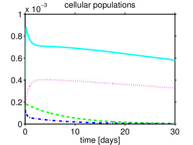
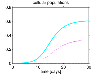
Figure 12. Temporal evolution of cellular populations and ECM in the perfused culture for $c_{\text{ext}}=c_{\text{sat}}$. Initial condition IC1. Left: $k_{\text{g}}=k_{\text{g1}}$. Right: $k_{\text{g}}=k_{\text{g2}}$. Solid line: $\phi_{\textrm{n}}$; dashed line: $\phi_{\textrm{v}}$; dotted line: $\phi_{\textrm{q}}$; dash-dot line: $\phi_{\textrm{ECM}}$.

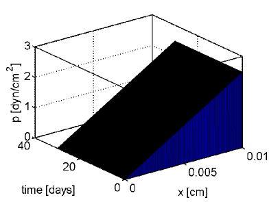
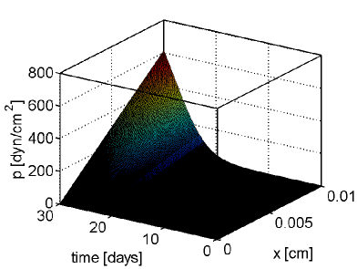
Figure 13. Spatial and temporal evolution of fluid pressure in the perfused culture for $c_{\text{ext}}=c_{\text{sat}}$. Initial condition IC1. Left: $k_{\text{g}}=k_{\text{g1}}$. Right: $k_{\text{g}}=k_{\text{g2}}$.

Figure 14. Spatial and temporal evolution of oxygen concentration in the perfused culture for $c_{\text{ext}}=c_{\text{sat}}$. Initial condition IC1. Left: $k_{\text{g}}=k_{\text{g1}}$. Right: $k_{\text{g}}=k_{\text{g2}}$.

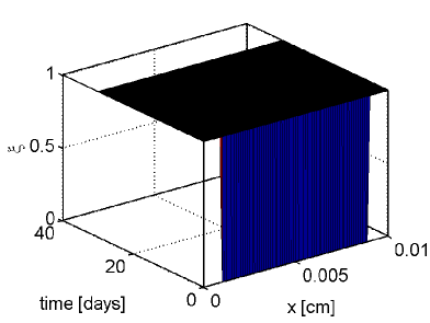
Figure 15. Spatial and temporal evolution of parameter $\xi$ in the perfused culture for $c_{\text{ext}}=c_{\text{sat}}$. Initial condition IC1. Left: $k_{\text{g}}=k_{\text{g1}}$. Right: $k_{\text{g}}=k_{\text{g2}}$.

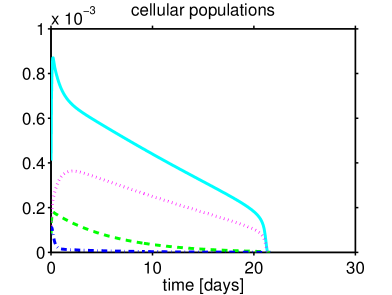
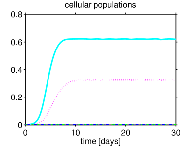
Figure 16. Temporal evolution of cellular populations and ECM in the perfused culture for $c_{\text{ext}}=c_{\text{thr}}$. Initial condition IC1. Left: $k_{\text{g}}=k_{\text{g1}}$. Right: $k_{\text{g}}=k_{\text{g2}}$. Solid line: $\phi_{\textrm{n}}$; dashed line: $\phi_{\textrm{v}}$; dotted line: $\phi_{\textrm{q}}$; dash-dot line: $\phi_{\textrm{ECM}}$.

Fig. 12 (left panel) clarifies how the mitotic activity is preponderant with respect to the other phases, that, differently, very quickly converge to zero. As a matter of fact proliferating cells, after the initial spike typical of the low growth regime, show a plateau-like behaviour that dramatically delays cell apoptosis. This result highlights the reaction of the system to the mechanical boundary conditions: the external force exerted by the fluid gives rise to an anisotropic stress state that instantaneously propagates throughout the domain, as shown in Fig. 15, maintaining the anisotropic mechanical configuration in both low and high growth regimes. This mechanical stimulus is the sole responsible of the strong mitotic functional activity occurring within the biomass and shown in Fig. 12 (left panel). As a matter of fact, as evidenced in Fig. 14, oxygen consumption is practically absent since nutrient concentration remains substantially unchanged except the very small sink in the case $k_{\text{g}}=k_{\text{g2}}$ at $x=0\,\mathrm{cm}$ and $t=15$ days.

The spatial and temporal evolution of the fluid pressure is displayed in Fig. 13. In the low growth regime (Fig. 13 left panel) fluid pressure shows a Darcy-like behavior and linearly increases along the spatial domain. On the contrary, in the high growth regime the evolution of the pressure becomes nonlinear and, at the end of the simulation at the rightmost end of the domain, it reaches a spike whose value is about two orders of magnitude larger than the maximum value in the low growth case. This happens because of the concurrence of two factors: first, at the right boundary of the domain an external positive pressure is applied, second, at the end of the simulation the porosity within the biomass decreases and, consequently, the fluid pressure dramatically increases.

Fig. 16 shows the response of cellular populations when the external nutrient level drops below the saturation threshold. If the maximum cell growth rate is not high enough, all cell populations rapidly decrease and disappear shortly after twenty days of simulation (left panel). This result proves that in a dynamical culture, when the external oxygen concentration is insufficient, cell survival is ensured only if the growth rate is large enough (right panel).

5.2.2. Initial condition IC2

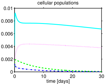
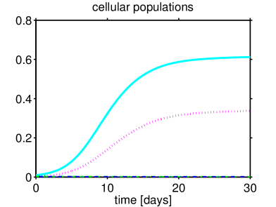
Figure 17. Temporal evolution of cellular populations and ECM in the perfused culture for $c_{\text{ext}}=c_{\text{sat}}$. Initial condition IC2. Left: $k_{\text{g}}=k_{\text{g1}}$. Right: $k_{\text{g}}=k_{\text{g2}}$. Solid line: $\phi_{\textrm{n}}$; dashed line: $\phi_{\textrm{v}}$; dotted line: $\phi_{\textrm{q}}$; dash-dot line: $\phi_{\textrm{ECM}}$.

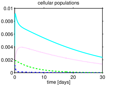
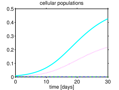
Figure 18. Temporal evolution of cellular populations and ECM in the perfused culture for $c_{\text{ext}}=c_{\text{thr}}$. Initial condition IC2. Left: $k_{\text{g}}=k_{\text{g1}}$. Right: $k_{\text{g}}=k_{\text{g2}}$. Solid line: $\phi_{\textrm{n}}$; dashed line: $\phi_{\textrm{v}}$; dotted line: $\phi_{\textrm{q}}$; dash-dot line: $\phi_{\textrm{ECM}}$.

Fig. 17 shows that at high seeding densities cell behavior does not undergo a significant variation, probably because in the perfused case the conditions for oxygen supply improve and oppose the negative consequences of a high crowding of cells. For this reason we present below only the computational results relative to the solid mixture components, since the other variables evolve in a very similar way as in the initial condition IC1. As shown in Fig. 18, the initial high seeding density guarantees the survival of biomass cellular component even in correspondence of a reduced level of oxygen concentration.

6. Discussion of simulation results

In this paper we developed the numerical approximation of the mathematical mechanobiological model introduced in Part I of this article. Despite the intrinsic simplicity of the one-dimensional formulation, the computational tests described in Sect. 5 constitute a useful validation of the biophysical consistency of the mechano-physiological model and a preliminary attempt toward a qualitative and quantitative prediction on the evolution of the construct components and, consequently, on the formation of the engineered tissue. Below we address the more significant outcomes of the conducted simulations.

1. The illustrated numerical results indicate that the in vitro cell cultivation process is strongly sensitive to variations of (i) the initial seeding density of cells, (ii) the value of the maximum growth rate and (iii) the mechanical boundary conditions. In particular, the amount of seeded cells turns out to be determinant for cell responsiveness: initial cell density should be high enough to ensure optimal conditions for proliferation, but not so high that grow factors are rapidly depleted from the medium and the contact inhibition phenomenon prevents the formation of new colonies (see Fig. 10). Furthermore the value of parameter $k_{\text{g}}$ influences the long-term behavior of the biomass. As a matter of fact, model simulations indicate that if $k_{\text{g}}$ is smaller than the reference value $k_{\text{g,0}}$, cell metabolic activity and ECM synthesis significantly decrease in the cultured construct and are completely exhausted at about 10 days of culture (Figs. 2 top, 6 left). On the contrary, model predictions show that if the maximum growth rate exceeds the reference value, cell and ECM volumetric fractions increase until convergence to a finite value that represents a stable steady state of the mathematical system (Figs. 2 bottom, 6 right). This finding represents a favorable result from the experimentalist point of view, because it predicts the formation, at the end of the cultivation and under specific conditions, of the bio-artificial texture to be used for replacing damaged tissues, that constitutes the real aim of TE. A similar objective can be reached by conveniently assigning the mechanical boundary conditions at the interface between the biomass construct and the interstitial fluid. As a matter of fact, model results indicate that when the biomass is stimulated by both external fluid velocity and pressure, even if $k_{\text{g}}$ is tuned on a under-threshold value, the amount of cells and ECM in the construct remains considerable until the end of the simulation (see Fig. 12 top panel). This outcome reinforces the notion that mechanical stimulation in perfused cultures may promote chondrogenesis and ECM production [24, 23, 7]. Actually, in order to achieve this optimal result, nutrient concentration at the fluid-biomass interface should not fall under a critical level otherwise cell functionality could be rapidly reduced until cell apoptosis (see Fig. 16 left panel).

2. The behavior of the solid mixture components is in excellent agreement with the experimental trends obtained by cultivation of engineered tissues in bioreactors. In particular, the temporal evolution of construct cellularity and ECM content, especially for an under-threshold value of $k_{\text{g}}$, agree with experimental results shown in several papers [32, 18, 7, 9].

3. The characterization of the (an)isotropicity of the biomass intrinsic stress state through the equivalent parameter $\xi$ introduced in (6c) demonstrated to be a successful strategy to model the mechanical regulation of culture progression and to link the mechanisms occurring at the micro-scale level to the macroscopic functioning of the growing tissue (see [15]). As a matter of fact, model predictions show that the parameter $\xi$ is an effective indicator of the propagation of the isotropic and anisotropic waves within the construct and allows an easy and immediate identification of the adhesion mechanisms developing at the single cell-level, that, accordingly, drive the evolution of the volumetric fraction $\phi_{\textrm{v}}$ and $\phi_{\textrm{n}}$ respectively.

7. Future perspectives

Below, we mention several future steps that we intend to take in the prosecution of this promising research activity.

1. A sensitivity analysis to provide the bio-scientist an indication of the critical values of the parameters that significantly perturb the cell cultivation fate. The analysis will be the object of a subsequent paper in which we will determine the homogeneous stable steady states of the model.

2. The introduction of a visco-elastic component in the constitutive law for the total stress with the purpose of damping out the propagation of the anisotropy/isotropy waves, as recently proposed in [1].

3. The inclusion of other mixture constituents, such as proteoglycan and collagen as done in [12].

4. The extension of the computational algorithms to treat a fully three-dimensional representation of the scaffold pore to allow a deeper model validation against previous existing simulation results and experimental data (see, e.g., [22, 8, 13]).

Symbol	Definition	Value	Units	Reference
$c_{0}$	$O_{2}$ concentration for $t=0$	$5\times 10^{-6}$	$\mathrm{g\;cm^{-3}}$	this work
$c_{\text{sat}}$	$O_{2}$ saturation concentration	$6.4\times 10^{-6}$	$\mathrm{g\;cm^{-3}}$	[5]
$c_{\text{thr}}$	$O_{2}$ threshold concentration	$1.6\times 10^{-6}$	$\mathrm{g\;cm^{-3}}$	[14]
$c_{\text{apo}}$	$O_{2}$ apoptosis concentration	$3.2\times 10^{-7}$	$\mathrm{g\;cm^{-3}}$	[14]
$K_{\mathrm{eq}}$	$O_{2}$ local mass equilibrium coefficient	$0.1$	-	[4]
$D_{\mathrm{c},\textrm{s}}$	$O_{2}$ diffusivity in the solid phase	$0.75\times 10^{-5}$	$\mathrm{cm^{2}\;s^{-1}}$	[4]
$D_{\mathrm{c},\textrm{fl}}$	$O_{2}$ diffusivity in the fluid phase	$1\times 10^{-5}$	$\mathrm{cm^{2}\;s^{-1}}$	[4]
$V_{b}$	inlet velocity of perfusion fluid	$50\times 10^{-4}$	$\mathrm{cm\;s^{-1}}$	[5]
$T_{b}$	stress due to perfusion fluid	$100$	$\mathrm{mPa}$	[5]
$\mu_{\textrm{fl}}$	fluid dynamic viscosity at $20^{\circ}$ C	$1.002\cdot 10^{-2}$	$\mathrm{g\;cm^{-1}\;s^{-1}}$	[10]
$R_{\textrm{n}}=R_{\textrm{v}}$	$O_{2}$ consumption rate for n/v-cells	$3.9\times 10^{-8}$	$\mathrm{g\;(cm^{3}\;s)^{-1}}$	[27]
$R_{\textrm{q}}$	$O_{2}$ consumption rate for q-cells	$10^{-8}$	$\mathrm{g\;(cm^{3}\;s)^{-1}}$	this work
$K_{1/2}$	$O_{2}$ half saturation constant	$3.2\times 10^{-6}$	$\mathrm{g\;cm^{-3}}$	[27]
$\beta_{{\rm A}\rightarrow{\rm B}}$	transition rate from state A to state B	$10^{-5}$	$\mathrm{s^{-1}}$	this work
$k_{\text{apo}}$	apoptosis transition rate	$3.858\times 10^{-7}$	$\mathrm{s^{-1}}$	[27]
$k_{\text{qui}}$	quiescence transition rate	$3.858\times 10^{-7}$	$\mathrm{s^{-1}}$	this work
$k_{\text{deg}}$	ECM degradation rate	$7.7\times 10^{-7}$	$\mathrm{s^{-1}}$	[31]
$k_{\text{g0}}$	maximum specific cell growth rate	$5.8\times 10^{-6}$	$\mathrm{s^{-1}}$	[27]
$k_{\text{g1}}$	”low” specific cell growth rate	$1\times 10^{-7}$	$\mathrm{s^{-1}}$	this work
$k_{\text{g2}}$	”high” specific cell growth rate	$1\times 10^{-5}$	$\mathrm{s^{-1}}$	this work
$E$	expansion coefficient	$20$		[5]
$k_{\text{GAG}}$	GAG synthesis rate	$8.61\times 10^{-11}$	$\mathrm{cm^{6}\;(cell\;s\;g)^{-1}}$	[5]
$K_{\text{sat}}$	Monod saturation constant	$1.927\times 10^{-6}$	$\mathrm{g\;cm^{-3}}$	[6]
$D_{\eta}$	cells and ECM diffusion coefficient	$1\times 10^{-9}$	$\mathrm{cm^{2}\;s^{-1}}$	this work
$\lambda_{\eta}$	cells and ECM Lamé’s parameter	$5.1937\times 10^{3}$	$\mathrm{dyne\,cm^{-3}}$	[28]
$\mu_{\eta}$	cells and ECM Lamé’s parameter	$1.8248\times 10^{3}$	$\mathrm{dyne\,cm^{-3}}$	[28]
$\phi_{\textrm{ECM},\mathrm{max}}$	maximum ECM volume fraction	$0.1$		this work
$R_{\text{cell}}$	cell radius	$5\times 10^{-4}$	$\mathrm{cm}$	this work
$V_{\text{cell}}$	cell volume	$5.236\times 10^{-10}$	$\mathrm{cm^{3}}$	this work
$\tau_{\text{m}}$	mitotic characteristic time	$172800$	$\mathrm{s}$	[29]
$K_{\text{ref}}$	reference permeability	$1.67\cdot 10^{-5}$	$\mathrm{cm^{3}s\;g^{-1}}$	this work

Table 1. Numerical values of model parameters used in the simulation tests.

References

- [1] L. Bociu, G. Guidoboni, R. Sacco, and J. T. Webster. Analysis of nonlinear poro-elastic and poro-visco-elastic models. Under Review in Archive for Rational Mechanics and Analysis, 2015.
- [2] F. Brezzi and M. Fortin. Mixed and Hybrid Finite Element Methods. Springer Verlag, New York, 1991.
- [3] A. N. Brooks and T. J.R. Hughes. Streamline Upwind/Petrov-Galerkin formulations for convection dominated flows with particular emphasis on the incompressible Navier-Stokes equations. Computer Methods in Applied Mechanics and Engineering, 32(12̆0133):199 – 259, 1982.
- [4] P. Causin and R. Sacco. A computational model for biomass growth simulation in tissue engineering. Communications in Applied and Industrial Mathematics, 2(1):1–20, 2011.
- [5] P. Causin, R. Sacco, and M. Verri. A multiscale approach in the computational modeling of the biophysical environment in artificial cartilage tissue regeneration. Biomechanics and Modeling in Mechanobiology, 12(4):763–780, 2013.
- [6] G. Cheng, P. Markenscoff, and K. Zygourakis. A 3D hybrid model for tissue growth: The interplay between cell population and mass transport dynamics. Biophys J., 97:401–414, 2009.
- [7] C. A. Chung, C. W. Chen, C. P. Chen, and C. S. Tseng. Enhancement of cell growth in tissue-engineering constructs under direct perfusion: Modeling and simulation. Biotechnology and Bioengineering, 97.
- [8] M. Cioffi, J. Kueffer, S. Stroebel, G. Dubini, I. Martin, and D. Wendt. Computational evaluation of oxygen and shear stress distributions in 3D perfusion culture systems: Macro-scale and micro-structured models. Journal of Biomechanics, 41(14):2918–2925, 2008.
- [9] T. Davisson, R. L. Sah, and A. Patcliffe. Perfusion increases cell content and matrix synthesis in chondrocyte three-dimensional cultures. Tissue Eng, 8:807–816, 2002.
- [10] F.P. Incropera and D.P. DeWitt. Fundamentals of heat and mass transfer. Wiley, 1990.
- [11] R. I. Issa, B. Engebretson, L. Rustom, P. S. McFetridge, and V. I. Sikavitsas. The effect of cell seeding density on the cellular and mechanical properties of a mechanostimulated tissue-engineered tendon. Tissue Engineering: Part A, 17:1479–1487, 2011.
- [12] S. M. Klisch, R. L. Sah, and A. Hoger. A cartilage growth mixture model for infinitesimal strains: solutions of boundary-value problems related to in vitro growth experiments. Biomech. Model. Mechanobiol., 3:209–223, 2005.
- [13] M. Laganà and M. T. Raimondi. A miniaturized, optically accessible bioreactor for systematic 3D tissue engineering research. Biomed. Microdevices, 14:225–234, 2012.
- [14] A. Mara and M. Nava. Modellizzazione multifisica del processo di rigenerazione tessutale all’interno di un bioreattore perfuso, 2011. Master Thesis, Politecnico di Milano.
- [15] M. M. Nava, R. Fedele, and M. T. Raimondi. Computational prediction of strain-dependent diffusion of transcription factors through the cell nucleus. Biomechanics and Modeling in Mechanobiology, pages 1–11, 2015.
- [16] M.M. Nava, M.T. Raimondi, and R. Pietrabissa. Controlling self-renewal and differentiation of stem cells via mechanical cues. Journal of Biomedicine and Biotechnology, 2012:12, 2012.
- [17] N.I. Nikolaev, B. Obradovic, H.K. Versteeg, G. Lemon, and D.J. Williams. A validated model of gag deposition, cell distribution, and growth of tissue engineered cartilage cultured in a rotating bioreactor. Biotechnol Bioeng., 105(4):842–853, 2010.
- [18] B. Obradovic, J. H. Meldon, L. E. Freed, and G. Vunjak-Novakovic. Glycosaminoglycan deposition in engineered cartilage: Experiments and mathematical model. AIChE J., 46 (9):1860–1871, 2000.
- [19] A. Quarteroni and A. Valli. Numerical Approximation of Partial Differential Equations. Springer-Verlag, New York, Berlin, 1994.
- [20] M. T. Raimondi. Engineered tissue as a model to study cell and tissue function from a biophysical perspective. Current Drug Discovery Technologies, 3(4):245–268, 2006.
- [21] M. T. Raimondi, F. Boschetti, L. Falcone, F. Migliavacca, A. Remuzzi, and G. Dubini. The effect of media perfusion on three-dimensional cultures of human chondrocytes: integration of experimental and computational approaches. Biorheology, 41:401–10, 2004.
- [22] M. T. Raimondi, F. Boschetti, F. Migliavacca, M. Cioffi, and G. Dubini. Micro fluid dynamics in three-dimensional engineered cell systems in bioreactors. In N. Ashammakhi and R. L. Reis, editors, Topics in Tissue Engineering, volume 2, chapter 9. 2005.
- [23] M. T. Raimondi, G. Candiani, M. Cabras, M. Cioffi, M. Laganà, M. Moretti, and R. Pietrabissa. Engineered cartilage constructs subject to very low regimens of interstitial perfusion. Biorheology, 45:471–8, 2008.
- [24] M.T. Raimondi, M. Moretti, M. Cioffi, C. Giordano, F. Boschetti, K. Laganà, and R. Pietrabissa. The effect of hydrodynamic shear on 3D engineered chondrocyte systems subject to direct perfusion. Biorheology, 43(3-4):215–222, 2006.
- [25] H. G. Roos, M. Stynes, and L. Tobiska. Numerical methods for singularly perturbed differential equations. Springer-Verlag, Berlin Heidelberg, 1996.
- [26] R. Sacco, L. Carichino, C. de Falco, M. Verri, F. Agostini, and T. Gradinger. A multiscale thermo-fluid computational model for a two-phase cooling system. Computer Methods in Applied Mechanics and Engineering, 282(0):239 – 268, 2014.
- [27] R. Sacco, P. Causin, P. Zunino, and M. T. Raimondi. A multiphysics/multiscale 2D numerical simulation of scaffold-based cartilage regeneration under interstitial perfusion in a bioreactor. Biomech Model Mechanobiol, 10(4):577–589, 2011.
- [28] G. De Santis, A. B. Lennon, F. Boschetti, B. Verhegghe, P. Verdonck, and P. J. Prendergast. How can cells sense the elasticity of a substrate? an analysis using a cell tendegrity model. European cells and Materials, 22:202–213, 2011.
- [29] B. G. Sengers, C. W. J. Oomens, and F. P. T Baaijens. An integrated finite-element approach to mechanics, transport and biosyntheis in tissue engineering. Journal of Biomechanical Engineering, 126(1):82–91, 2004.
- [30] M. A. Soltz and G. A. Ateshian. Experimental verification and theoretical prediction of cartilage interstitial fluid pressurization at an impermeable contact interface in confined compression. J. Biomech., 31(10):927–934, 1998.
- [31] A. J. Trewenack, C. P. Please, and K. A. Landman. A continuum model for the development of tissue-engineered cartilage around a chondrocyte. Mathematical Medicine and Biology, 26:241–262, 2009.
- [32] G. Vunjak-Novakovic, B. Obradovic, I. Martin, P. M. Bursac, R. Langer, and L. E. Freed. Dynamic cell seeding of polymer scaffolds for cartilage tissue engineering. Biotechnology Progress, 14(2):193–202, 1998.