An alternative order-parameter for non-equilibrium generalized spin models on honeycomb lattices

Abstract

An alternative definition for the order-parameter is proposed, for a family of non-equilibrium spin models with up-down symmetry on honeycomb lattices, and which depends on two parameters. In contrast to the usual definition, our proposal takes into account that each site of the lattice can be associated with a local temperature which depends on the local environment of each site. Using the generalised voter motel as a test case, we analyse the phase diagram and the critical exponents in the stationary state and compare the results of the standard order-parameter with the ones following from our new proposal, on the honeycomb lattice. The stationary phase transition is in the Ising universality class. Finite-size corrections are also studied and the Wegner exponent is estimated as $\omega=1.06(9)$.

I Introduction

For equilibrium systems, the universality hypothesis allows to cast all critical systems in universality classes, of which the Ising model universality class is the best-known example. The concept of universality can be extended to non-equilibrium critical systems Henkel et al. (2008); Täuber (2014). In particular, a widely accepted conjecture states that non-equilibrium models with up-down symmetry and spin-flip dynamics fall in the universality class of the Ising model Grinstein et al. (1985). A family of generalized spin models (GSM) that do not satisfy the detailed-balance condition and which present a non-equilibrium steady-state, was proposed by Oliveira et al. de Oliveira et al. (1993); Tomé and de Oliveira (2014). The collective behaviour of the “spins” shares many aspects with the well-established theory of non-equilibrium phase transitions and results from simulations can be analysed similarly Henkel et al. (2008). In these GSM, the system evolves following a competing dynamics induced by heat baths at two different temperatures (on two-dimensional square lattices) Droz et al. (1989); Tamayo et al. (1994); Drouffe and Godrèche (1999) and hence have a non-equilibrium stationary state. In the original version of the GSM de Oliveira et al. (1993), each lattice site is occupied by a spin, $\sigma_{i}$, that interacts with its nearest neighbours. The system evolves in the following way: during an elementary time step, a spin $\sigma_{i}=\pm 1$ on the lattice is randomly selected, and flipped with a probability given by

$$p=\frac{1}{2}[1-\sigma_{i}f(H_{i})],$$ (1)

where $H_{i}$ is the local field produced by the nearest neighbours to the site $i$ and $f(H_{i})$ is a local function bounded by $|f(H_{i})|\leq 1$. On a square lattice, one habitually uses one of two possible sets of parameters, such that

$$f(H_{i})=\left\{\begin{array}[]{l}f(2)=-f(-2)=x=\tanh(2\beta_{2})\\ f(0)=0\\ f(4)=-f(-4)=y=\tanh(4\beta_{4})\end{array}\right.$$ (2)

The dynamics is described by two parameters: either the pair ($x,~{}y$) which act analogously to a noise in the system, or else by a pair of effective inverse temperatures ($\beta_{2},~{}\beta_{4}$) de Oliveira et al. (1993); Drouffe and Godrèche (1999). In the second case, to each site one associates a “temperature” that depends on its instant local environment. This locally fluctuating “temperature” should affect the model’s macroscopic behaviour. Several known models are known special cases of the dynamics eqs. (1,2): the majority voter model (MVM) corresponds to $y=x$ or $\beta_{2}=2\beta_{4}$; the Glauber-Ising model (GIM) corresponds to $y=2x/(1+x^{2})$ or $\beta_{2}=\beta_{4}$. Numerical simulations confirm that these models, on a square lattice, belong to the Ising model universality class de Oliveira (1992); de Oliveira et al. (1993); Kwak et al. (2007); Wu and Holme (2010). In this work, we propose a new order-parameter with the following features: (i) it must take into account that the local variable has extra degrees of freedom because there is not just one heat bath involved, and (ii) it must recover the standard Ising model when the heat baths are at the same temperature. Additionally, we can introduce in this way a new model of out of equilibrium mixed-spin models, similar to the ferrimagnetic models (see Z̆ukovic̆ and Bobák (2015) and references therein).

This work is organised as follows: in section II we described how to implement the new order parameter on the honeycomb lattice. In section III, the finite-size scaling method used to analyse its stationary state is outlined. In section IV, the results of the Monte Carlo simulation for a particular case, the equivalent MVM, are reported and the critical parameters are extracted. We conclude in section V.

II Model

In analogy with simple Ising magnets the paramagnetic-ferromagnetic phase transition can be measured with the standard order-parameter, on a square lattice $\Lambda\subset\mathbb{Z}^{2}$, with $N=L^{2}=|\Lambda|$ sites

$$\langle m\rangle=\frac{1}{N}\left\langle\left|\sum_{i\in\Lambda}\sigma_{i}\right|\right\rangle,$$ (3)

In this work, we propose an alternative definition for an order parameter, as follows

$$\langle\mu\rangle=\left\langle\left(\sum_{i\in\Lambda}\beta_{H_{i}}\right)^{-1}\left|\sum_{i\in\Lambda}\beta_{H_{i}}\sigma_{i}\right|\right\rangle.$$ (4)

such that the value of the inverse temperature $\beta_{H_{i}}$ is selected on each site, depending on the local field $H_{i}$, according to eq. (2). Certainly, when $\beta_{2}=\beta_{4}$, one should recover $\langle\mu\rangle=\langle m\rangle$. However, on lattices where each site has an even number of nearest neighbours, the order parameter $\langle\mu\rangle$ is not uniquely defined, since for configurations with a local field $H_{i}=0$ at the site $i$, a further un-specified parameter $\beta_{0}$ must be introduced. A work-around is to consider lattices where sites have an odd number of nearest neighbours, such as the honeycomb lattice (see Fig. 1). For the honeycomb lattice, the available values for the local field are $H_{i}=\pm 1,~{}\pm 3$ and the extra parameter $\beta_{0}$ is no longer needed.

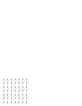
Figure 1: Honeycomb lattice used for the simulations, with this geometry we use use skew boundary conditions at the horizontal boundary.

On the honeycomb lattice, eq. (2) is replaced by

$$f(H_{i})=\left\{\begin{array}[]{l}f(1)=-f(-1)=x=\tanh(\beta_{1})\\ f(3)=-f(-3)=y=\tanh(3\beta_{3})\end{array}\right.$$ (5)

Again, we recover some known models: the MVM corresponds now to $x=y$ and $\beta_{1}=3\beta_{3}$ and the GIM corresponds to $y=(3x+x^{3})/(1+3x^{2})$ or $\beta_{1}=\beta_{3}$. Analogously we can define the susceptibility for the new order parameter as

$$\chi=Nx\{\langle\mu^{2}\rangle-\langle\mu\rangle^{2}\}.$$ (6)

For a qualitative illustration of the difference between the two order parameters, in Fig. 2 we present snapshots along the line $x=y$ for three different values of $x$ for a lattice of size $L=200$. The left column a) corresponds to the ordered phase, the central column b) to the critical point and the right column c) to the disordered phase. While the standard order parameter $\langle m\rangle$ permits to distinguish between the ordered and disordered phases, our new proposal $\langle\mu\rangle$ clearly hints at further hidden structures. For example, in the ordered phase, most sites have a local temperature $\beta_{3}$, whereas in the disordered phase, most sites have a local temperature $\beta_{1}$.

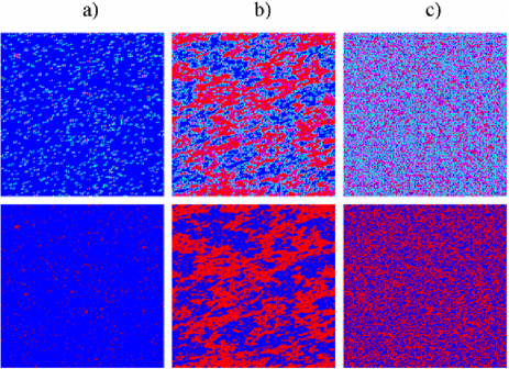
Figure 2: (Colour online) Snapshots of the honeycomb lattice of size $L=200$ along the line $y=x$, for a) $x=0.95$ b) $x=0.8720$ and c) $x=0.20$. The upper row corresponds to the new order parameter $\langle\mu\rangle$, see (4). Sites with a local spin $\sigma_{i}\beta_{H_{i}}=[+\beta_{3},~{}+\beta_{1},~{}-\beta_{1},~{}-\beta_{3}]$ are represented with colours [blue, cyan, magenta, red], respectively. The lower row corresponds to the standard order parameter $\langle m\rangle$, see (3). Sites with spin $\sigma_{i}=[+1,~{}-1]$ are represented by colours [blue,red], respectively. The order-parameter values are a) $\langle m\rangle\simeq 0.943,~{}\langle\mu\rangle\simeq 0.928$, b) $\langle m\rangle\simeq 0.052,~{}\langle\mu\rangle\simeq 0.040$ and c) $\langle m\rangle\simeq 0.009,~{}\langle\mu\rangle\simeq 0.007$.

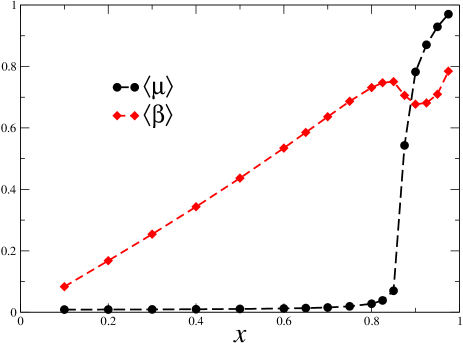
Figure 3: (Colour online) Dependence of the order-parameter $\langle\mu\rangle$ and of the average inverse temperature $\langle\beta\rangle$ on the coupling $x$ in the MVM, on the honeycomb lattice with $L=100$.

In figure 3, we illustrate the dependence of the averaged order-parameter $\langle\mu\rangle$ on the coupling $x$ in the MVM. Clearly, the existence of a second-order phase transition is signalled, very analogous to what one has found for the usual order-parameter $\langle m\rangle$ de Oliveira (1992); de Oliveira et al. (1993). On the other hand, considering the average inverse temperature $\langle\beta\rangle$ hints at additional structure not captured by $\langle m\rangle$. Curiously, there is a cusp in $\langle\beta\rangle$ which occurs very closely to the location $x_{c}$ of the critical point. While the increase of $\langle\beta\rangle$ with $x$ in the disordered phase should mainly reflect the dependence of $\beta_{1}$ on $x$, the cusp could be related to the increase of sites with an inverse temperature $\beta_{3}=\frac{1}{3}\beta_{1}$, as is also suggested by the snapshots in figure 2.

Since both the MVM and the GIM present a continuous phase-transition, it is natural to assume that a critical line should exist in the $x-y$ plane. In analogy to the square lattice case, this line starts at the voter critical point, $(x,y)=(1/3,1)$ for the honeycomb lattice, and ends at the extremal value $(x,y)\approx(1,0.88)$. In order to sketch the critical line, we carried out rough simulations with small lattice sizes, $L=24,28,32$ and $36$, at different fixed $x$ values. In order to estimate the critical points, we used the standard method of the crossing point of the fourth-order Binder cumulant Binder (1981)

$$U^{(4)}=1-\frac{\langle\mu^{4}\rangle}{3\langle\mu^{2}\rangle^{2}}.$$ (7)

For both order parameters (3,4) simulations were carried out by starting with a random configuration of spins, and letting the system evolve according to the dynamics given by eqs. (1,5). In figure 4, we show the phase diagram as estimated in the plane $(x,y)$ for the honeycomb lattice. Skew boundary conditions in the horizontal direction and periodic boundary conditions in the vertical direction were used, see Figure 1. In all cases, the uncertainties in the critical values are around $10^{-3}$. Clearly, we see from Figure 4 that the critical boundaries estimated from both order-parameters are compatible (see also table 1).

Table 1: Rough estimates of the critical points as found from the order parameters $m$ and $\mu$, respectively, for the honeycomb lattice. We also included the points $(x,y)=(0.57735027,0.96225045)$, common to both, $(x,y)=(0.8721,0.8721)$ for $m$ Acuña-Lara et al. (2014), and $(x,y)=(0.87195,0.87195)$ for $\mu$, as evaluated in next section.

$x$	$y_{c}~{}(m)$	$y_{c}~{}(\mu)$
0.500	0.982	0.982
0.550	0.970	0.970
0.600	$-$	0.956
0.650	$-$	0.941
0.700	0.925	0.925
0.750	0.909	0.908
0.800	$-$	0.891
0.850	0.880	0.875
0.900	0.866	0.864
0.950	0.861	0.858
0.999	$-$	0.879
1.000	0.884	$-$

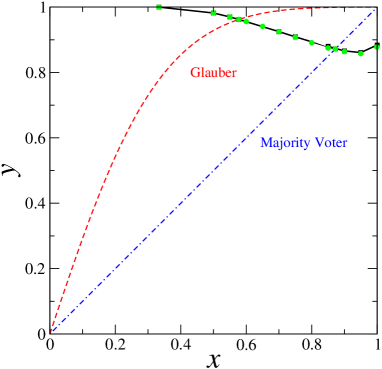
Figure 4: (Colour online) Phase diagram in the $(x,y)$ plane. The ordered phase is in the right upper zone and is separated from the disordered phase by the critical line, black solid line for $\langle m\rangle$ and green circles for $\langle\mu\rangle$. The red dashed line correspond to the Ising model and the point-dashed blue line correspond to the MVM.

III Finite-size scaling technique

We shall use the method proposed in Ref. Pérez (2005), where three different cumulants are used for the evaluation of the critical point: (i) the fourth-order or Binder cumulant, Eq. (7), (ii) the third-order cumulant (where $\langle\mu^{3}\rangle$ is defined analogously to eq. (4))

$$U^{(3)}=1-\frac{\langle\mu^{3}\rangle}{2\langle\mu\rangle\langle\mu^{2}\rangle},$$ (8)

and (iii) the second-order cumulant

$$U^{(2)}=1-\frac{2\langle\mu^{2}\rangle}{\pi\langle\mu\rangle^{2}}.$$ (9)

The scaling forms for the thermodynamic observables, in the stationary state, and together with the leading finite-size correction exponent $\omega$ (or Wegner’s exponent), are given by

$$\mu(\epsilon,L) \approx L^{-\beta/\nu}(\hat{M}(\epsilon L^{1/\nu})+L^{-\omega}\hat{\hat{M}}(\epsilon L)),$$ (10)

$$\chi(\epsilon,L) \approx L^{\gamma/\nu}(\hat{\chi}(\epsilon L^{1/\nu})+L^{-\omega}\hat{\hat{\chi}}(\epsilon L)),$$ (11)

$$U^{(p)}(\epsilon,L) \approx \hat{U}^{(p)}(\epsilon L^{1/\nu})+L^{-\omega}\hat{\hat{U}}^{[p]}(\epsilon L).$$ (12)

where $\epsilon=x-x_{c}$ is the distance from criticality, $p=2$, $3$ or $4$. The parameters $\beta$, $\gamma$ and $\nu$ are the critical exponents for the infinite system, see Henkel et al. (2008) for details.

In principle, the critical point $x_{c}$ is found from the crossing points in the cumulants $U^{(p)}$. A precise estimation of $x_{c}$ is achieved by taking into account the crossing points for different cumulants $U^{(p)}$ and $U^{(q)}$ with $p\neq q$ arise for different values of $L$. The values of $x$, where the cumulant curves $U^{(p)}(x)$ for two different linear sizes $L_{i}$ and $L_{j}$ intercept are denoted as $x^{(p)}_{ij}$. We expand Eq. (12) around $\epsilon=0$ to obtain

$$U^{(p)}\approx U^{(p)}_{\infty}+\bar{U}^{(p)}\epsilon L^{1/\nu}+\bar{\bar{U}}^{(p)}L^{-\omega}+{\rm O}(\epsilon^{2},\epsilon L^{-\omega}),$$ (13)

where $U^{(p)}_{\infty}$ are universal quantities, but $\bar{U}^{(p)}$ and $\bar{\bar{U}}^{(p)}$ are non-universal. The value of $\epsilon$ where the cumulant curves $U^{(p)}$ for two different linear sizes $L_{i}$ and $L_{j}$ intercept is denoted as $\epsilon^{(p)}_{i,j}$. At this crossing point the following relation must be satisfied:

$$L_{i}^{1/\nu}\epsilon^{(p)}_{ij}+B^{(p)}L_{i}^{-\omega}=L_{j}^{1/\nu}\epsilon^{(p)}_{ij}+B^{(p)}L_{j}^{-\omega}.$$ (14)

Here $B^{(p)}:=\bar{\bar{U}}^{(p)}/\bar{U}^{(p)}$. Combining for different cumulants ($q\neq p$) we get

$$\frac{x^{(p)}_{ij}+x^{(q)}_{ij}}{2}=x_{c}-(x_{ij}^{(p)}-x_{ij}^{(q)})A_{pq},$$ (15)

where $A_{pq}=(B^{(p)}+B^{(q)})/[2(B^{(p)}-B^{(q)})]$ and is non-universal (see Refs. Pérez (2005); Acuña-Lara and Sastre (2012) for additional details). Equation (15) is a linear equation that makes no reference to $\nu$ or $\omega$ and requires as inputs only the numerically measurable crossing couplings $x_{i,j}^{p}$. The intercept with the ordinate gives the critical point location.

IV Results

For the determination of the critical point and the critical exponents for the MVM, we performed simulations on lattices with linear sizes $L=24$, 32, 40, 48, 60, 76 and $96$, following the procedure used for the evaluation of the critical line of section II. We let the system evolve during a transient time, that varied from $4\times 10^{5}$ Monte Carlo time steps (MCTS) for $L=24$ to $1.5\times 10^{6}$ MCTS for $L=96$. Averages of the observables were taken over $1\times 10^{6}$ MCTS for $L=24$ and up to $1.5\times 10^{7}$ MCTS for $L=96$. Additionally, for each value of $x$ and $L$, we performed 300 (bigger lattices) to 500 (smaller lattices) independent runs, in order to improve the statistics.

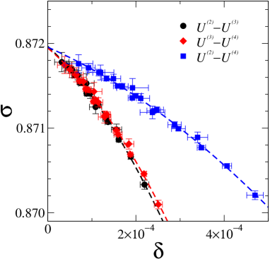
Figure 5: (Colour online) Evaluation of the critical point $x_{c}$. The points represent the numerical data obtained from third-order polynomial fits and the dashed lines are second-order polynomial fits of Eq. (15). Smaller $\delta$-values correspond to larger system sizes.

For the evaluation of the critical points, we used a third-order polynomial fit for the cumulant curves. Recalling eq. (15), the estimation of the critical point is shown in Figure 5, where we plot the variable $\sigma:=(x_{ij}^{(4)}+x_{ij}^{(2)})/2$ over against the variable $\delta:=x_{ij}^{(4)}-x_{ij}^{(2)}$. We observe that the curves $\sigma(\delta)$ are not linear as expected from Eq. (15), this means that the finite-size effects are significant in this case and the curvature is due to the neglected higher order terms in Eq. (12). When we compare the data for the crossing of the $U^{(2)}-U^{(4)}$ curves with the previous reported data for the standard order parameter given by Eq. (3) from Ref. Acuña-Lara et al. (2014), the range in the differences $\delta$ is almost two times larger with this new order parameter (see Fig. 2c in Ref. Acuña-Lara et al. (2014)) and that the smallest difference is around $7\times 10^{-5}$ (corresponding to the crossing between $L=96$ and $L=76$). When we compare with results for the antiferromagnetic MVM on honeycomb lattices (Figure 4b on reference Sastre and Henkel (2016)) we observe that the scaling effect, like the range in the differences $\delta$ and the departure from the linear behavior of $\sigma(\delta)$, are more notorious with the new order parameter. With the second order polynomial fits of Eq. (15) we obtain the result for the critical point of

$$x_{c}=0.87195(22)$$ (16)

where the number in brackets give the estimated uncertainty in the last given digit(s). This results is in good agreement with the reported value for the critical point of the standard order parameter for the ferromagnetic and antiferromagnetic MVM on honeycomb lattice Acuña-Lara et al. (2014); Sastre and Henkel (2016).

Once that we have the critical point, we can also analyse eventual finite-size corrections, which are described in terms of Wegner’s correction-to-scaling exponent $\omega$, which was already defined in eqs. (10-12). We evaluate the Wegner exponent $\omega$ and the universal quantities $U_{\infty}^{(p)}$ by using a non linear fit with (12) and $\epsilon=0$.

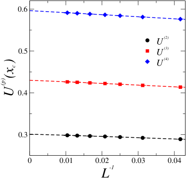
Figure 6: (Colour online) Cumulant values at the critical point as function of the inverse linear size. The dashed lines are non linear fits of Equation (12).

Again, we can observe that the scaling effects are more pronounced here, compared to the antiferromagnetic case with the standard order parameter on the same lattice (see Figure 8b in Sastre and Henkel (2016)). Our estimated value for the Wegner exponent is

$$\omega=1.06(9)$$ (17)

The usual prediction for $\omega$, based on $2D$ conformal invariance Henkel (1999); Caselle et al. (2002); Izmailian (2011) gives $\omega=2$ for the Ising model, on a square lattice with periodic boundary conditions. Early suggestions that $\omega$ might be as small as $4/3$ have been disproved numerically, in favour of $\omega=2$ Blöte and den Nijs (1988). However, in certain cases the corresponding amplitude may vanish and this leads to an effective value $\omega=4$, as seen for the Ising model on honeycomb and triangular lattices de Queiroz (2000). For open boundary conditions or Brascamp-Kunz boundary conditions, one rather finds $\omega=1$ Salas (2002); de Queiroz (2011); Janke and Kenna (2002). Finally, on the triangular lattice, effective values in the range $1.2\lesssim\omega_{\rm eff}\lesssim 2$ were reported Guo et al. (2005).

The values for the cumulants are $U_{\infty}^{(2)}=0.301(6)$, $U_{\infty}^{(3)}=0.430(7)$ and $U_{\infty}^{(4)}=0.597(7)$; they are all compatible with the reported values for the antiferromagnetic MVM on honeycomb lattices with the same boundary conditions Sastre and Henkel (2016).

The critical exponents can be evaluated, by using Eqs. (12), at the critical point $\epsilon=0$. One expects the following finite-size scaling behaviour

$$m(L) \sim L^{-\beta/\nu}(1+a_{m}L^{-\omega}),$$ (18)

$$\chi(L) \sim L^{\gamma/\nu}(1+a_{\chi}L^{-\omega}),$$ (19)

and

$$\frac{\partial U^{(p)}}{\partial x}\Bigl{|}_{x=x_{c}}\sim L^{1/\nu}(1+a_{U^{(p)}}L^{-\omega}),$$ (20)

where the correction-to-scaling exponent, with the value $\omega=1.06$, must be included, since the correction-to-scaling effects are important in this case. The parameters $a_{\alpha}$ are non-universal. In Fig. 7, we show the derivatives of the cumulants at the critical point. From the finite-size scaling law (20), we obtain the following results: $1/\nu=0.97(4)$, 0.99(4) and 0.99(3) from $\partial U^{(2)}/\partial x$, $\partial U^{(3)}/\partial x$ and $\partial U^{(4)}/\partial x$, respectively. After combining our results we finally obtain $1/\nu=0.98(4)$, in good agreement with the result for the two-dimensional Ising model. The evaluation of $\gamma/\nu$ is shown in Fig. 8, with the relation (19) we obtain $\gamma/\nu=1.75(2)$. We present in Fig. 9 the evaluation of $\beta/\nu$, with Eq. (18) we obtain $\beta/\nu=0.128(5)$.

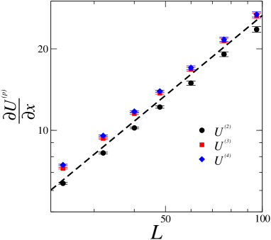
Figure 7: (Colour online) Log-log plot of the derivatives of the cumulants $U^{(2)}$, $U^{(3)}$ and $U^{(4)}$ with respect to $x$, taken at the critical point $x=x_{c}$. The dashed line show the expected power-law behaviour in the $L\to\infty$ limit for $1/\nu=0.98$.

Figure 8: Log-log plot of the susceptibility at the critical point. The dashed line show the expected power-law behaviour in the $L\to\infty$ limit for $\gamma/\nu=1.75$.

Figure 9: Log-log plot of the order parameter at the critical point. The dashed line show the expected power-law behaviour in the $L\to\infty$ limit for $\beta/\nu=0.128$.

All reported numerical estimates are very close to the exactly known values of the two-dimensional Ising ferromagnet, e.g. (Henkel et al., 2008, appendix A).

V Conclusions

We have introduced a new definition of an order-parameter for a family of generalized spin models in honeycomb lattices. This definition (4) of the new order parameter $\mu$ can be extended to other lattice types with an odd number of nearest neighbours. We studied through intensive Monte Carlo simulations the stationary state for a particular case that corresponds to the Majority voter model. We have found that the phase-diagram for this order-parameter in the two-parameter space $(x,y)$ is equivalent to the phase diagram for the standard order parameter, in both ferromagnetic and antiferromagnetic versions of the MVM. Furthermore, the estimated critical exponents

$$\frac{1}{\nu}=0.98(4),\quad\frac{\gamma}{\nu}=1.75(2),\quad\frac{\beta}{\nu}=0.128(5)$$ (21)

of the stationary state are, as expected, compatible to the ones of the $2D$ Ising model universality class. One important difference with respect to the previous numerical studies concerns the the correction-to-scaling effects. Their analysis permits to estimate the Wegner exponent $\omega$. Our result $\omega_{\rm MVM}=1.06(6)$ is not compatible with the conventional value $\omega_{\rm Ising}=2$ of the two-dimensional Ising model. Such small values of $\omega$ have usually been reported on certain non-periodic lattices in the $2D$ Ising model Salas (2002); de Queiroz (2000); Janke and Kenna (2002) while here, it arises as a result of the chosen dynamics. The only other known value for the MVM is for the three-dimensional cubic lattice Acuña-Lara and Sastre (2012); in this case the value of $\omega$ is compatible with the value of the Ising model. Further simulations should be performed in order to test further whether there is a new correction exponent for this model.

Finally, the use of $\mu$ might offer a finer view on the mechanism of a phase transition, see figures 2 and 3, and probably can be extended beyond the Ising model. We hope to return elsewhere to further exploration of new insights, especially in the context of non-equilibrium phase transitions.

References

- Henkel et al. (2008) M. Henkel, H. Hinrichsen, and S. Lübeck, Non-equilibrium phase transitions, vol I: absorbing phase transitions (Springer, Heidelberg, 2008).
- Täuber (2014) U. C. Täuber, Critical Dynamics (Cambridge University Press, Cambridge, 2014).
- Grinstein et al. (1985) G. Grinstein, C. Jayaprakash, and Y. He, Phys. Rev. Lett. 55, 2527 (1985).
- de Oliveira et al. (1993) M. J. de Oliveira, J. F. F. Mendes, and M. A. Santos, J. Phys. A: Math. Gen. 26, 2317 (1993).
- Tomé and de Oliveira (2014) T. Tomé and M. J. de Oliveira, Dinâmica estocástica e irreversibilidade (2a edição) (Livraria de Física, São Paulo, 2014).
- Droz et al. (1989) M. Droz, Z. Rácz, and J. Schmidt, Phys. Rev. A39, 2141 (1989).
- Tamayo et al. (1994) P. Tamayo, F. J. Alexander, and R. Gupta, Phys. Rev. E50, 3474 (1994), eprint [arXiv:cond-mat/9407046].
- Drouffe and Godrèche (1999) J.-M. Drouffe and C. Godrèche, J. Phys. A: Math. Gen. 32, 249 (1999), eprint [arXiv:cond-mat/9807356].
- de Oliveira (1992) M. J. de Oliveira, J. Stat. Phys. 66, 273 (1992).
- Kwak et al. (2007) W. Kwak, J.-S. Yang, J.-i. Sohn, and I.-m. Kim, Phys. Rev. E75, 061110 (2007).
- Wu and Holme (2010) Z.-X. Wu and P. Holme, Phys. Rev. E 81, 011133 (2010), eprint [arXiv:0911.0049].
- Z̆ukovic̆ and Bobák (2015) M. Z̆ukovic̆ and A. Bobák, Physica A436, 509 (2015), eprint [arXiv:1412.5811].
- Binder (1981) K. Binder, Zeitschrift für Physik B43, 119 (1981).
- Acuña-Lara et al. (2014) A. Acuña-Lara, F. Sastre, and J. Vargas-Arriola, Phys. Rev. E89, 052109 (2014), eprint [arXiv:1401.4632].
- Pérez (2005) G. Pérez, Journal of Physics: Conference Series 23, 135 (2005).
- Acuña-Lara and Sastre (2012) A. Acuña-Lara and F. Sastre, Phys. Rev. E86, 041123 (2012), eprint [arXiv:1208.6521].
- Sastre and Henkel (2016) F. Sastre and M. Henkel, Physica A444, 897 (2016), eprint [arXiv:1509.04598].
- Henkel (1999) M. Henkel, Conformal Invariance and Critical Phenomena (Springer, Heidelberg, 1999).
- Caselle et al. (2002) M. Caselle, M. Hasenbusch, A. Pelissetto, and E. Vicari, J. Phys. A: Math. Gen. 35, 4861 (2002), eprint [arXiv:cond-mat/0106372].
- Izmailian (2011) N. Izmailian, Phys. Rev. E84, 051109 (2011).
- Blöte and den Nijs (1988) H. Blöte and M. den Nijs, Phys. Rev. B37, 1766 (1988).
- de Queiroz (2000) S. de Queiroz, J. Phys. A: Math. Gen. 33, 721 (2000), eprint [arXiv:cond-mat/9912090].
- Salas (2002) J. Salas, J. Phys. A. Math. Gen. 35, 1833 (2002), eprint [arXiv:cond-mat/0110287].
- de Queiroz (2011) S. de Queiroz, Phys. Rev. E84, 031107 (2011), eprint [arXiv:1105.6248].
- Janke and Kenna (2002) W. Janke and R. Kenna, Phys. Rev. B65, 064110 (2002), eprint [arXiv:cond-mat/0103332].
- Guo et al. (2005) W. Guo, H. Blöte, and Z. Ren, Phys. Rev. E71, 046126 (2005).