∎
11institutetext: Martin Delacourt (Corresponding author)22institutetext: CMM, Universidad de Chile, CNRS, Av. Blanco Encalada 2120, Santiago, Chile
33institutetext: Benjamin Hellouin de Menibus44institutetext: CMM, Universidad de Chile, CNRS, Av. Blanco Encalada 2120, Santiago, Chile
Departamento de Matemáticas, Universidad Andres Bello, Chile
Characterisation of limit measures
of higher-dimensional cellular automata††thanks: Research partially supported by the FONDECYT Postdoctorado Proyecto 3130496 and by Basal project No. PFB-03 CMM, Universidad de Chile
Abstract
We consider the typical asymptotic behaviour of cellular automata of higher dimension (). That is, we take an initial configuration at random according to a Bernoulli (i.i.d) probability measure, iterate some cellular automaton, and consider the (set of) limit probability measure(s) as . In this paper, we prove that limit measures that can be reached by higher-dimensional cellular automata are completely characterised by computability conditions, as in the one-dimensional case. This implies that cellular automata have the same variety and complexity of typical asymptotic behaviours as Turing machines, and that any nontrivial property in this regard is undecidable (Rice-type theorem). These results extend to connected sets of limit measures and Cesàro mean convergence. The main tool is the implementation of arbitrary computation in the time evolution of a cellular automata in such a way that it emerges and self-organises from a random configuration.
Keywords:
Symbolic dynamics Cellular automata Limit measure Multidimensional ComputabilityCellular automata are discrete dynamical systems defined by a local rule, introduced in the 40s by John von Neumann Neumann . They model a large variety of discrete systems and are linked with various areas of mathematics and computer science, in particular computation theory, complex systems, ergodic theory and combinatorics.
One of the main catalysts of the study of cellular automata was their surprisingly complex and organised behaviours, even when iterated on configurations with no particular structure (e.g. chosen at random). To formalise these observations, many authors tried to describe their asymptotic behaviour by considering the limit set, which is the set of configurations that can be reached after arbitrarily many steps. These sets were shown to have potentially high computational complexity Maass-1995 ; Ballier-Guillon-Kari-2011 , and any nontrivial property on them is undecidable Kari-1994 . These observations built a bridge between the variety of dynamical behaviours and the computational content of the model. Nevertheless, the problem of characterising which sets can be limit sets of CA remains open.
In 2000, Kůrka and Maass argued that limit sets did not provide a good description of empirical observations and introduced instead a measure-theoretical version of these sets km-2000 . The idea of -limit sets is to choose the initial configuration at random, according to some probability measure , to iterate the cellular automaton on this configuration and to consider all patterns whose probability to appear does not tend to 0. In the one-dimensional case, this approach yielded similar results of high complexity and undecidability bpt-2006 ; Boyer-Delacourt-Sablik-2010 ; Delacourt-2011 ; bdpst . Although these two families of results appear similar and both require sophisticated constructions inside cellular automata, they provide insight about different kinds of dynamics (topological vs. measure-theoretical) and computational power (deterministic vs. probabilistic).
In HellouinSablik , H. and Sablik extended this approach to consider the limit probability measure(s). Still in the one-dimensional case, they provided a computational characterisation of the limit measures reachable by cellular automata, generalising the previous results.
This article is an extended version of Delacourt-Hellouin . In op.cit, we aimed at extending the previous results to the two-dimensional setting. More precisely, we characterised all subshifts that can be -limit sets of CA when is the uniform Bernoulli measure. The proof works by an explicit construction inspired by the one-dimensional constructions of bdpst ; HellouinSablik , although the higher dimensional setting has many specific challenges. In the present article, this two-dimensional construction is generalised to a -dimensional space for any ; furthermore, through a more careful analysis, we are able to characterise reachable limit measures, which is a more general result. As a corollary, we obtain an undecidability result on properties of limit measures, and cover as well Cesàro mean convergence and the case where the limit measure is not unique.
Section 1 is devoted to general definitions. In Section 2, we introduce more specific computability tools, and in particular computability restrictions on possible limit probability measures. In Section 3, we describe, process by process, the main technical construction that is the core of the proof of our results. Section 4 contains the main results that are the corollaries of this construction, mainly:
Theorem 0.1 (Main result)
The measures for which there exist:
-
•
an alphabet ,
-
•
a cellular automaton , and
-
•
a non-degenerate Bernoulli measure
such that , are exactly the limit-computable measures.
This result holds even when the initial measure is chosen to be uniform. As a corollary, we show that any nontrivial property on limit measures is undecidable. These result extend to connected sets of limit measures and convergence in Cesàro mean.
1 Definitions
1.1 Symbols, configurations and cellular automata
Let be a finite set of symbols called alphabet. For , let be the space of -dimensional configurations.
On , we define the basis vectors (Kronecker deltas), that is, the vector worth on all coordinates except the -th where it is worth . Denote and the set of hyperplanes that have a normal vector in ; these hyperplanes have a basis of vectors in .
We will use the following distances between points of :
An -path is a sequence of points such that for any . An -connected set is a subset of such that any pair of points are connected by an -path. Define similarly -paths and -connected subsets.
If we endow with the product topology of the discrete topology on , then is a Cantor set (compact, perfect and totally disconnected). This topology is also metrisable, for example using the Cantor metric:
For a subset , denote the restriction of to . Denote the set of finite patterns. For a pattern , denote its support , and its dimension is the smallest such that is isomorphic to a subset of . We say a pattern is cubic, respectively rectangular, if its support is a , resp. a (Cartesian product of intervals).
The cylinder defined by a pattern and a position is . For simplicity we sometimes write for .
The shift map, or shift, is defined as:
A subshift is a closed subset of invariant under all shifts. Given a cubic pattern , define the periodic configuration by and for every .
A cellular automaton (or CA) is a continuous function that commutes with all shifts ( for every ). By the Curtis-Hedlund-Lyndon theorem Hedlund , it can be defined equivalently as a function where is a finite set called neighbourhood and is called a local rule.
1.2 Probability measures on
Let be the Borel -algebra of and the set of probability measures on defined on the -algebra . In this article, we focus on the set of -invariant probability measures on , that is to say, the measures such that for all and . Cylinders corresponding to finite patterns form a base of the topology. Since for any and , is entirely characterised by ; actually, considering only cubic patterns is enough.
We endow with the weak∗ (or weak convergence) topology:
In the weak∗ topology, is compact and metrisable. A metric is defined by
Define the ball centred on of radius as
Let us define some examples that we use throughout the article.
The Bernoulli measure associated to some vector satisfying is defined by
The Dirac measure supported by is defined as . Generally is not -invariant. However, for any cubic pattern , it is possible to define the -invariant measure supported by by taking the mean of the Dirac measures on the orbit under :
The set of measures is dense in Petersen-1983-livre .
1.2.1 Action of a cellular automaton on and limit measures
Let be a cellular automaton and . Define the image measure by for all . Since is -invariant, that is to say , one deduces that . This defines a continuous application .
We consider in particular the iterated image of by . Since is compact in the weak topology, the sequence admits a set of limit points denoted and called the -limit set of measures of . When is a singleton, i.e. when , we say is the limit measure of starting on .
This name stems from the standard -limit set of defined as .
2 Computability
We now introduce the computability notions that are needed to state our main results. This exposition is very similar to the one found in HellouinSablik , which was later expanded in These , for the one-dimensional case. Indeed, most of the definitions and proofs only rely on the fact that the space is metric and separable, properties for which the increase in dimension is irrelevant. We omit those proofs that can be obtained by a straightforward substitution () from the proofs found in these references.
2.1 Turing machines
Turing machines are a standard and robust tool to define the computability of mathematical operations. In the usual model, they have access to a one-dimensional, one- or two-sided infinite memory tape. In order to simplify some constructions, we consider in this article that the tape is -dimensional and infinite in all directions. This does not affect the computing power of the model.
A Turing machine is defined by:
-
•
a finite alphabet, with a blank symbol . Initially, a -dimensional infinite memory tape is filled with , except for a finite region (the input), and a computing head is located at coordinate ;
-
•
a finite set of states, with an initial state ;
-
•
the transition function. Given the current state and the letter it reads on the tape — which depends on its current position — the function returns the new state, the letter to be written on the tape at current position, and the vector by which the head moves.
-
•
the set of final states — when a final state is reached, the computation stops and the output is the contents of the tape.
A function is computable if there exists a Turing machine working on an alphabet that, on any input , eventually stops and outputs .
2.2 Computability of functions mapping countable sets
To generalise this definition to functions mapping arbitrary countable sets , we need to define an encoding, that is, an alphabet together with a bijection between and some subset of , and similarly for . Then the computability of a function is defined up to some encoding. However, in practice, reasonable encodings yield the same notion of computability. To simplify notations, we fix some canonical encodings for the rest of the paper :
- (or ):
-
Take and encode an element as its binary expansion surrounded by blank symbols.
- Product :
-
Take and encode as the product of encodings for and .
Using this last case, we define a canonical encoding for as the canonical encoding for , up to the bijection (with irreducible).
Furthermore, we define the computability of a set as the computability of the function .
2.3 Computability of probability measures
As we mentioned above, a probability measure is entirely described by the value of for all . In other words, an element of is described by a function . Since is not countable, the standard ways to define notions of computability is to consider approximations by elements of .
A measure is computable if there exists a computable function such that
It is limit-computable if there exists a computable function such that
Additionally we define the notion of a uniformly computable sequence. Informally, it means that a sequence of objects can be computed by a single algorithm which, given as input, returns a description of the -th object of the sequence.
Formally, a sequence of measures is uniformly computable iff there exists a computable function such that:
It is easy to see that the limit of a uniformly computable sequence of measures is limit-computable (but not necessarily computable since the rate of convergence of to is not known).
Proposition 1 (Approximation by measures supported by periodic orbits)
These notions can be defined in another equivalent way:
-
(i)
A measure is computable if and only if there exists a computable function such that for all .
-
(ii)
A measure is limit-computable if and only if there exists a computable function such that .
Notice the parallel with the definition of the computability of a real: in both cases, an object is computable if it is approximated by a uniformly computable sequence of elements taken from a dense subset ( and the measures supported by periodic orbits, respectively) with a known rate of convergence.
2.4 Action of a cellular automaton on computable measures
Proposition 2 (First computability obstruction)
Let be a cellular automaton and be a computable measure. Then is a uniformly computable sequence of measures. In particular, if then is limit-computable.
In general, does not have a single limit point, but a compact set of accumulation points. To obtain a similar obstruction, we extend our computability definitions to those objects.
2.5 Compact sets in computable analysis
Extending naively the definition for countable sets using the characteristic function does not work since the set of inputs would not be countable. Instead, we use a general definition for metric spaces that possess a countable dense subset, in the case of .
A closed set is computable if the set is computable (as a countable set), that is, if its characteristic function is.
However, the set of limit points of the sequence , where is computable, is not necessarily computable (or even limit-computable). We extend our definitions to the first steps of the so-called arithmetical hierarchy, first on countable spaces, then on closed subsets of .
Let be two countable sets, with being ordered.
A sequence of functions is uniformly computable if is computable.
A function is -computable (resp. -computable) if (resp. ), where is a uniformly computable sequence of functions.
A closed set is -computable if the set
is -computable, that is, its characteristic function is.
Remark 1
The symmetric notions of - and -computability come from an analogy with the real arithmetical hierarchy Zheng-Weihrauch-2001 ; Ziegler-2005 . These definitions extend naturally to - and -computability. Other equivalent definitions exists, see for example HellouinSablik for -computability or These for a more general result.
Proposition 3 (Second computability obstruction)
Let be a cellular automaton and be a computable measure. Then is a nonempty -computable compact set.
Aiming at a reciprocal, notice that -computable compact sets can be all be described as the set of limit points of a sequence of measures , where the sequence of patterns is uniformly computable. However, our construction cannot do better that following such a sequence along a polygonal path, that is, along segments of the form . The following proposition shows that this corresponds to connected limit sets of measures (not necessarily path-connected).
Proposition 4 (Technical characterisation of -CCC sets)
Let be a non-empty -computable, compact, connected set (-CCC for short). Then there exists a uniformly computable sequence of cubic patterns such that is the limit of the polygonal path defined by , that is,
As we mentioned before, the proof of these statements can be found in HellouinSablik or These for an extended version.
3 Construction
To obtain the results announced in the introduction, we prove the following result in conjunction to Proposition 4.
Theorem 3.1
For any uniformly computable sequence of cubic patterns of of dimension at most , there exists a larger alphabet and a cellular automaton such that for any Bernoulli measure :
In the rest of the article, assume some fixed alphabet and some uniformly computable sequence of patterns of . We present the construction of the alphabet and cellular automaton .
3.1 Sketch of the construction
We detail the construction of and by describing the tasks to be performed on the initial configuration. Each letter of is a product of seven layers separated in three groups, each group representing some information needed to perform a given task. The alphabet of each layer contains a special blank symbol to denote the absence of information.
-
•
The first group is dedicated to the colonising of the configuration. Since we have no control over the contents of the initial configuration, we want to erase (almost) all symbols present initially in favour of various processes that we can control and synchronise. To do this, the birth layer contains a seed symbol
![[Uncaptioned image]](/html/1512.03696/assets/x1.png) that can only appear in the initial configuration. Each seed gives birth to a stationary heart
that can only appear in the initial configuration. Each seed gives birth to a stationary heart
![[Uncaptioned image]](/html/1512.03696/assets/x2.png) on the same layer, and to a membrane on the growth layer which grows in every direction. As it grows, the membrane erases everything in its path, except for other membranes issued from a seed with which it merges.
on the same layer, and to a membrane on the growth layer which grows in every direction. As it grows, the membrane erases everything in its path, except for other membranes issued from a seed with which it merges. -
•
The second group is used to divide the colonised space into mostly independent areas called organisms, each organism having at its centre a heart issued from a seed. The borders between organisms are redefined regularly by processes on the organism layer. Furthermore, organisms need to grow in size regularly, which is achieved by merging organisms whose hearts are close using the evolution layer.
-
•
The third group deals with the internal metabolism of the organisms. The goal is first to compute each in succession, which is achieved by simulating a Turing machine in the computing layer; then, the main layer of the whole body of the organism is filled with concatenated copies of by using a copying process taking place on the copying layer. The above is done synchronously in all organisms, at some time for each .
Copies of are written on the main layer, which implies that the corresponding alphabet is . To sum up, the global alphabet is . We check that up to the bijection . Denote , , , , , , the projections on each coordinate.
During the description of , we will treat each layer successively. The layers were introduced in order of dependency, in the sense that the time evolution of symbols in a given layer only depends on the contents of layers in the same group and the one immediately preceding it. Furthermore, the main layer is only affected by the copying layer.
3.2 Space colonisation: Seeds and membranes
In this section, we describe the cleaning of the configuration through the seeds and the birth, growth and fusion of membranes. We deal only with the birth layer and alphabet for the moment. Section 3.2.1 gives the general ideas of the process, while Section 3.2.2 focuses on technical difficulties of the cellular implementation.
3.2.1 Creation myth: a sketch
Seeds and hearts
The alphabet contains the seed symbol
![]() , which can only appear in the initial configuration and cannot be produced by the local rule of . At the first step, each seed spawns a number of processes and turns into a heart . This heart and those processes (and those spawned from them) are called initialised, which means that their behaviour is well controlled and synchronised (since they are all born at time ). All other symbols are uninitialised.
, which can only appear in the initial configuration and cannot be produced by the local rule of . At the first step, each seed spawns a number of processes and turns into a heart . This heart and those processes (and those spawned from them) are called initialised, which means that their behaviour is well controlled and synchronised (since they are all born at time ). All other symbols are uninitialised.
If two seeds are too close from each other ( less than 5), the largest (in lexicographic order) is erased to give enough space to the other seed to spawn its processes. A seed that is not destroyed at time in this way is called viable. By abuse of notation we write to mean that the configuration has a viable seed at coordinate .
Birth of membranes
Each occurrence of
![]() triggers the birth at time of a living membrane. The membrane consists in membrane symbols
triggers the birth at time of a living membrane. The membrane consists in membrane symbols
![]() and
and
![]() (and all their rotations) that form initially the surface of an hypercube of edge length centred on the seed. The membrane is oriented, being able to distinguish inside from outside through orientation vectors.
(and all their rotations) that form initially the surface of an hypercube of edge length centred on the seed. The membrane is oriented, being able to distinguish inside from outside through orientation vectors.
Definition 1
A membrane at time is a maximal -connected set of coordinates containing membrane symbols
![]() or
or
![]() at time with consistent outward orientation; i.e., orientation of neighbouring membrane symbols differ in at most one coordinate, and at most by .
at time with consistent outward orientation; i.e., orientation of neighbouring membrane symbols differ in at most one coordinate, and at most by .
When a membrane forms a closed curve (which is the case for initialised membranes), we denote its support. In this case, partitions into a finite set and an infinite set which are -connected. We also denote . By "outward" in the previous definition, we mean that the orientation vectors of are directed towards .
If a membrane has a malformation that can be detected locally around a symbol (e.g. no neighbours, inconsistent orientations), a death process is spawned. Since uninitialised membranes can be locally well-formed, this is not enough to discriminate them from initialised membranes.
Breathing, growing, getting older
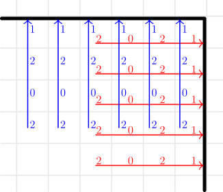
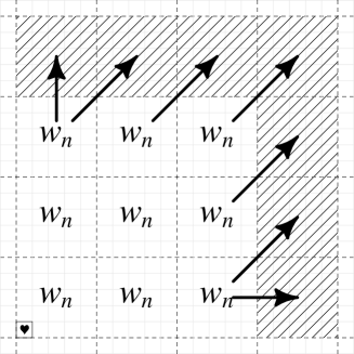
Each membrane symbol is associated with an age counter, which is a binary counter initialised at and increasing at each step, whose aim is to keep track of the value of . Notice that in an initialised membrane all age counters are equal. Figure 2 represents some part of a membrane with arrows and counters.
From time onward, the membrane grows slowly towards the outside, erasing the content of other layers as it progresses with the exception of other membranes (see next paragraph). This is governed by the respiration process: each time the age stored in its counter is the square of an integer, the membrane grows to the outside, making one step in every direction. Technical details related to the implementation of age counters and the respiration process are the object of the next section.
Fight for survival and death
When the growing membranes meet other membrane symbols, they try to determine locally whether they are part of an initialised membrane (in which case the two should merge), or some uninitialised symbols which should be erased. We call dead an uninitialised group of membrane symbols that present some locally detectable malformation, such as non-connexity, the absence of or inconsistencies between age counters/respiration processes, inconsistencies between inner and outer orientation for neighbours, etc. In this case, the malformation generates a death signal
![]() that spreads through the whole membrane erasing it. However, such a group can also form a zombie membrane, that is apparently well-formed though uninitialised. Initialised (living) and zombie membranes are distinguished through age counters.
that spreads through the whole membrane erasing it. However, such a group can also form a zombie membrane, that is apparently well-formed though uninitialised. Initialised (living) and zombie membranes are distinguished through age counters.
Fact 1
At time , all age counters associated with a well-formed membrane have value at least , the minimum being reached only for initialised membranes.
Indeed, age counters of initialised membranes are initialised at at time , while age counters of zombie membranes were already present (with a positive value) at time , and both are incremented by at each step.
3.2.2 Implementation of age counters
This section is dedicated to the details of the cellular implementation of the age counters in the growth layer. First we show how to implement age counters with binary counters using logarithmic space. contains membranes symbols and age counter symbols. Each membrane symbol
![]() or
or
![]() contains an outward orientation label consisting of a vector of .
contains an outward orientation label consisting of a vector of .
Basis and carry propagation
We use a redundant binary basis in all counters. Let be a counter. The value of is (reverse order) where has value . Since , 2 can be seen as a with a carry, and as a with a "negative" carry.
At each time step, carries are propagated along the counter, which can be done in a local manner (). Additional zeroes at the beginning of the counter are erased ().
In order to increment or decrement the counter by one, which is the case for age counters, the rule is adapted at the least significant bit of the counter (for incrementing: ).
Age counters
The age counters are implemented as follows. The least significant bit of each counter is next to its corresponding membrane symbol, and the following bits lie on a line directed towards the inside of the membrane. To each possible direction (corresponding to some ) corresponds a different sublayer, which allows counters to cross near the corners. Thus the age counters use sublayers, each sublayer containing symbols .
Recall that any inconsistency – the absence of an age counter for some membrane symbols, parallel counters containing different symbols, etc. – spawns a death process, which spreads in the whole membrane and erases all layers of these cells.
3.2.3 The respiration process
The goal of the respiration process is to govern a slow growth of the membrane.
Breathing counters
Along with the age counter, on two other sublayers of , two counters and are initialised at time with values and , respectively. From there on three phases alternate, the current phase being labelled on the membrane symbol:
- Phase :
-
is decremented while is incremented. When reaches , the phase passes to ;
- Phase :
-
is incremented while is decremented. When reaches , the membrane breathes;
- Breath:
-
For one step is incremented while is unchanged, then the phase passes to .
The value of is constant during a cycle ( for the first cycle) except for the last step where it is incremented by one. The cycle takes a total time . Therefore a breath occurs at each time for . In Figure 3 we represent the update operation of all three counters, that is, incrementing the age and updating and according to the phase.
Lemma 1
The counter update can be performed locally with radius .
Proof
The incrementations and decrementations described above can be achieved with radius . The least significant bit can be distinguished by being next to the membrane symbol which contains the information on the current phase and the most significant bit is next to a blank symbol (on its layer).
We show that the fact that a counter is worth is detectable with radius (to see why this is nontrivial, consider the update ). During a decrementation the least significant bit alterns between and . Since carries progress at "speed" one, two negative carries can never be next to each other. Therefore the only possible representations of are and , and both yield at the next step. Therefore detecting when the counter is worth requires radius two, in order for the membrane symbol to "see" the word . ∎
Breathing process
Each breath makes the membrane progress by one cell on every direction, a process we detail below. If such a symbol is not produced synchronously by the whole membrane, then
![]() signals spawn and spread to erase the membrane.
signals spawn and spread to erase the membrane.
Recall that each membrane symbol at coordinates is labelled with an outward growth direction, which is a vector . The membrane symbol is the border between and , with the orientation vector indicating which part is. When a breath symbol appears, the membrane symbol is removed and new symbols are created on all cells of that were -adjacent to any membrane symbol of . The new orientation vectors are determined by remaining coherent with the old orientation.
The remaining task is to reproduce the counters for the new symbols.
First consider the case of a face symbol and orientation . Right after a breath, when a new symbol is created at coordinate , the symbol at is replaced by a placeholder symbol . This symbol progressively shifts the counters of by one cell in direction , marking at each step the limit between the part which is to be shifted and the part already shifted. The counters keep updating by ignoring this symbol, which increases the radius to 3. Figure 4 illustrates the shift.

From this section we deduce the following:
Fact 2
Each initialised membrane forms an hypercube of edge length at time .
Since the counters of an initialised membrane are initialised to at time , the maximum size of the counters is at time and membranes have enough space to contain them. For technical reasons that will become clear later, we need to quantify the maximal number of breaths of any membrane symbol (not necessarily initialised) in a given time:
Lemma 2
The number of breaths triggered by any membrane symbol between times and is at most .
Proof
Apart from time (when a breath symbol could be present), a breath is only triggered when the B counter of a membrane symbol without local malformations reaches . This symbol must be issued from a seed or from a membrane symbol already present at time . In the first case, since a breath is triggered at each step when the time is the square of an integer (except for ), the number of breaths before time is . The lemma follows.
In the second case, the membrane symbol had at time counters and with some positive values and and some phase , values which correspond to those of an initialised set of counters at some time . From there on the time evolution of the membrane symbol is similar to the evolution of an initialised membrane symbol of age , which means that the number of breaths between times and is . ∎
Forming colonies
For an initial configuration , define to be the set of initialised membranes at time . Then the colonised space at time is:
When a membrane grows, it erases the content of every other layer of the cells it encounters, except when the birth layer contains the outer border of a membrane. In this case, the comparison process starts, which is the topic of the next section.
To sum up, the alphabet contains seeds and hearts, and contains the states used for membranes (including counter sublayers). As we will see in the next section, different membranes can share the same cell, so this alphabet will be duplicated this many times.
3.2.4 Survival of the youngest
As membranes grow and tend to cover the whole space, different membranes eventually meet. The result of the encounter should depend on the nature of the membranes: two initialised membranes should merge while an initialised membrane should erase an uninitialised membrane (what happens between uninitialised membrane is irrelevant). In this section, we devise a comparison process to distinguish initialised from uninitialised membranes, using the growth layer and its alphabet .
From Fact 1 we know that initialised membranes have the youngest age counters, and only tie with other initialised membranes. The value of the age counters are compared to let the younger membrane survive, with merging occurring in case of equality.
Many membranes meeting
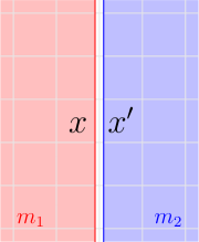
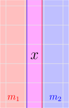
When we say that two membranes and meet at time in cells and , we mean that there exists such that:
-
•
either , and , in which case take ;
-
•
or and , in which case take .
The two possible situations are illustrated in Figure 5.
 |
 |
In particular, the membranes arriving from opposite directions, they have (at least) an age counter in opposite directions, say and . These age counters are to be copied on a dedicated sublayer of and compared.
Copying phase
At positions and , two symbols
![]() and
and
![]() are written on the growth layer to trigger the process (if , a symbol
are written on the growth layer to trigger the process (if , a symbol
![]() represents the superposition of those symbols) and progress at speed one in the corresponding direction, copying at each step one bit from the age counter to a sublayer of . Carries are copied as : indeed, the copy is performed at the same speed as the carry progresses, so it would be copied at each step otherwise (the carry is taken into account once it turns a into a ). More generally, only carries that appeared before the beginning of the copy can influence the copied counter, which is not incremented. Thus the copied counter have the same value as the age counter at the beginning of the copy. When it reaches the end of its counter, each copy symbol turns into a comparison symbol
represents the superposition of those symbols) and progress at speed one in the corresponding direction, copying at each step one bit from the age counter to a sublayer of . Carries are copied as : indeed, the copy is performed at the same speed as the carry progresses, so it would be copied at each step otherwise (the carry is taken into account once it turns a into a ). More generally, only carries that appeared before the beginning of the copy can influence the copied counter, which is not incremented. Thus the copied counter have the same value as the age counter at the beginning of the copy. When it reaches the end of its counter, each copy symbol turns into a comparison symbol
![]() (resp.
(resp.
![]() ), which triggers the comparison phase.
), which triggers the comparison phase.
Comparison phase
The comparison symbols return towards the meeting point, "pushing" the copied bits in front of them in a caterpillar-like movement, starting from the most significant bit. The returning bits use another sublayer of . The process is represented in Figure 6.
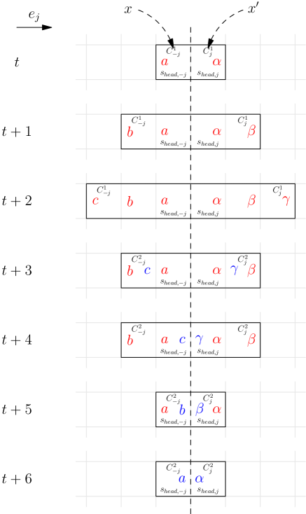
As the returning bits reach the meeting point, one of the following situations occur:
-
•
the most significant bit from one side arrives earlier than the most significant bit from the other side. In this case the age counter of the corresponding side is shorter, which means that the membrane of this side is younger;
-
•
both most significant bits arrive simultaneously at the meeting points and . Then bits are compared as they arrive. The first bit that is smaller than its counterpart corresponds to the side of the younger membrane;
-
•
in the previous case, if all bits are equal until the end, both membranes have exactly the same age.
Those three possibilities are tested locally at the meeting point and the result is written as a symbol (on its own sublayer) marking the direction of the younger membrane, with in case of a tie. If for some reason a symbol
![]() (death process) reaches the symbol of one of the sides, the comparison stops and the surviving membrane is marked as younger "by default".
(death process) reaches the symbol of one of the sides, the comparison stops and the surviving membrane is marked as younger "by default".
If a membrane is declared younger, all auxiliary symbols used for comparison are erased and a death process triggers in the older membrane. The younger membrane will resume its growth naturally at the next breath. If the result is a tie, both membrane symbols are erased along with all associated auxiliary states: the membranes are merged.
Remark 2
-
•
In general two membranes may have more than one meeting point. In that case, comparisons are performed simultaneously at every point and in every concerned direction. In the case of a tie, all symbols participating in the meeting are erased simultaneously; any local discrepancy results in the spawn of a death process.
-
•
At most different membranes can meet in the same cell (corners of hypercubes arriving from all possible directions). To solve this problem, we duplicate each sublayer (in and ) used in the comparison into copies, each copy being able to perform a comparison independently of the others. If the membrane is older than at least another membrane, a death process is spawned; it merges if it is tied for youngest.
-
•
Let be the length of the shortest age counter. The previous process needs steps to copy this age counter on the growth layer, and steps to send them one by one to the meeting point. Regardless of the length of the other counter, the comparison reaches a result after the last bit of the shortest counter arrives. Therefore the whole process takes at most steps. Remember that if one of the membranes is initialised (assuming the comparison process began at time ).
Breathing during comparisons
We did not take into account the possibility that one of the membranes breathes during the comparison. For each meeting of a pair of membranes, call instigating membrane the one whose breath has triggered the meeting (possibly both if they moved simultaneously; this is the case for initialised membranes).
Lemma 3
Let be a living membrane meeting another membrane at time . During the comparison process, may breath at most one time if it is not instigating, and cannot breath at all if it is instigating.
Proof
Using the above remark, we know that the comparison process takes at most steps. Using Lemma 2, the number of breaths of between times and is at most:
If is instigating, then by definition breathed at time and cannot breath again before time . Otherwise, breathes at most one time. ∎
Therefore, if one or both membranes move during the comparison because of the respiration process, it writes a head symbol to recall its new position. If a membrane extends more than twice before the end of the comparison, a death process is triggered for this membrane. As the radius of is more than , the moved membrane can still read the result of the comparison.
Lemma 4
Take any and initial configuration . Then:
In other words, the colonised space at time is exactly the set of cells that, at time , are at distance less than from a viable seed.
Proof
We prove this result by structural induction. If , then the colonised space is the set of all initialised membranes which are hypercubes of edge side around each viable seed, and the result is proved.
Now suppose that the hypothesis holds at time . Notice than , and that merging does not add any cell to the colonised space: an initialised membrane cannot be erased, and the colony obtained after merging two membranes is the union of the colonies defined by the two merged membranes. Only the breathing process may add new cells to the colonised space.
Consequently, the induction step is empty if is not a square since and (distances are integers). If is a square, then all membrane symbols in initialised membranes take a breath and extend by one cell towards the outside. Now, take a cell at distance from the nearest viable seed. By the induction hypothesis, , but has a neighbour with at distance from that seed, so that . Therefore must be a membrane symbol in the support of an initialised membrane that breathes at time , and therefore . Conversely, if a cell is at distance greater than from the nearest viable seed, it cannot have a membrane symbol belonging to an initialised membrane as a neighbour, so that .
∎
3.3 Colonies: evolution of the population
From Lemma 4 we can see that only the contents of the colonised space matter asymptotically. In this section, we describe the interaction of organisms inside colonies. In all the following, we assume we are inside a colony, and the support of the surrounding membrane acts as an impassable wall for any symbol in the second group layers: the organism and evolution layers.
3.3.1 Hearts and organisms
As we saw, seeds
![]() at time spawn a membrane and turn into hearts
at time spawn a membrane and turn into hearts
![]() . Each heart will be the centre of an organism which is itself a subset of the colony. At first each colony have only one heart, but as initialised membranes merge together, the colonies become multi-hearted, and the colony space is partitioned into organisms (except possibly a negligible part). For various reasons, the size of the organisms should grow in a controlled way, which requires some hearts to be progressively removed.
. Each heart will be the centre of an organism which is itself a subset of the colony. At first each colony have only one heart, but as initialised membranes merge together, the colonies become multi-hearted, and the colony space is partitioned into organisms (except possibly a negligible part). For various reasons, the size of the organisms should grow in a controlled way, which requires some hearts to be progressively removed.
In the present section, we present the cycle of division of colony space and life of the organisms, and all symbols presented here belongs to .
The life of an organism consists in a succession of generations. We introduce a sequence of times (to be fixed later), marking the limit between the -th and -th generation. Time is tracked by the heart through a binary time counter similar to age counters, initialised at at time (along with the heart) and remaining stationary next to the heart. Details on the implementation and the way to determine when will be given in Section 3.4.1.
Organisms expanding
At each time , organism-building signals spread from every heart, progressing as membrane symbols but with speed (although they do not carry any counters). While progressing, they erase the old contents of the second and third group layers except for the main layer. When they meet a membrane or another organism-building signal, they vanish leaving behind a neutral border symbol
![]() . For parity reasons, if two signals emitted by hearts in and arrive simultaneously in two neighbour cells and , they leave behind two pseudo-border symbol
. For parity reasons, if two signals emitted by hearts in and arrive simultaneously in two neighbour cells and , they leave behind two pseudo-border symbol
![]() with an orientation vector towards the interior of their organism, that is, the direction opposite to the initial organism-building signal.
Just as membrane symbols, different organism-building symbols and pseudo border symbols are required (one for each orientation).
with an orientation vector towards the interior of their organism, that is, the direction opposite to the initial organism-building signal.
Just as membrane symbols, different organism-building symbols and pseudo border symbols are required (one for each orientation).
The territory of a heart is the maximal set of -connected cells containing the heart and no neutral border symbol
![]() nor pseudo border symbol pointing towards another organism; in other words, the set of cells reached first by organism-building signals emitted by this heart. At time (assuming ), the only cells of the colony that are not part of some organism are either at distance more than from the nearest heart, or were outside the membrane at time (and a breath had included them since).
nor pseudo border symbol pointing towards another organism; in other words, the set of cells reached first by organism-building signals emitted by this heart. At time (assuming ), the only cells of the colony that are not part of some organism are either at distance more than from the nearest heart, or were outside the membrane at time (and a breath had included them since).
Fact 3
Let be a cell containing a heart at time with , and let be a cell in its territory. Then the organism-building signal emitted by reached at time and no other organism-building signal reached a neighbour of before that time.
The following lemma gives insight about the shape of the territories, namely, that they are a (discrete) star domain, whether the borders are included or not.
Lemma 5
If a cell belongs to the territory of a heart in cell , then each cell such that is also in this territory. Furthermore, can be a border only if is a border.
Proof
For the first part of the lemma, suppose such a is not in the territory of . We can build an -path between and consisting of cells such that . Take the first that belongs to the territory of .
Denote the time when the organism-building signal emitted by should have reached in the absence of any other heart. Since is not in the territory of , there must exist another heart that emitted an organism-building signal that arrived in before time (recall that the pseudo-borders are considered as parts of organisms).
Since is adjacent to , is reached by some signal before time . But the signal from cannot reach before time . Therefore is not in the territory of , a contradiction.
For the second case, notice that is a border if and only if both signals reached this cell simultaneously. Then the same reasoning along the path shows that these cells cannot be inside the territory of . ∎
3.3.2 Natural selection
In this section we consider the evolution layer and the alphabet .
To have enough computation space and ensure that the auxiliary symbols are in negligible density, the minimal size of the organisms should grow regularly. More precisely, we require that the territory of any organism during the -th generation contains at least a hypercube of side length centred at its heart. If two hearts are at distance less than , they are said to be in conflict. In this section, we devise a selection process to detect this fact and to erase one of them.
The first lemma is related to the quantity and position of hearts conflicting with a given heart.
Definition 2
For each point and each vector that is not we introduce the corresponding quadrant defined as .
For , each quadrant contains a unique -extremal point, which is a point such that for all . Denote the set of its directions of extremality relative to . Notice that this notion is defined for any vector such that .
Lemma 6
At any given generation, a heart conflicts with at most one other heart in each quadrant. In particular, it conflicts with at most hearts.
Proof
Let be the position of the heart and the current time. The heart in conflicts with another heart at if and only if . If two conflicting hearts were in the same quadrant, then they would be at distance at most , a contradiction. The bound is tight and reached by the configuration where there is a heart per quadrant at each -extremal point relative to the heart in . ∎
Settling conflicts at random
Each heart keeps in memory a random central bit and the winner of each conflict is decided through the value of these bits: if the bits are equal, destroy the largest heart (in lexicographic order), and the smallest otherwise. As long as the central bits of all hearts are independent of each other, this process will ensure that the probability of each heart to be destroyed in any conflict has a constant lower bound that only depends on the initial Bernoulli.
Remark 3
In dimension HellouinSablik ; bdpst , the heart in the smallest cell was systematically killed. The reason why we adopt a more sophisticated kill choice method, similar to the one used in Delacourt-Hellouin , is that we later need to control the growth rate of the organisms. This growth rate analysis under the simpler method proved to be more difficult than in dimension and could not be carried out.
Independent bit harvesting
In addition to its central bit, each heart maintains a collection of side bits, one for each quadrant, that must remain independent of each other and of every other central or side bits of other hearts. This is achieved by using the independence of the initial measure. At time , each seed looks at its adjacent cells (which are in one-to-one correspondence with its quadrants): if a cell contains the symbol
![]() (the symbol choice is arbitrary) then the corresponding bit in the newborn heart is put to , and otherwise. Remember that if two seeds are too close, one is erased, hence those bits are really independent from one another and from other hearts.
(the symbol choice is arbitrary) then the corresponding bit in the newborn heart is put to , and otherwise. Remember that if two seeds are too close, one is erased, hence those bits are really independent from one another and from other hearts.
Each time a heart kills another in a conflict, the dying heart transmits one of his side bits to its killer (the bit corresponding to which quadrant the killer belongs to). The new central bit of the killer is the sum of the side bits received from its victims. As we will see, this process lets us maintain probability bounds on the value of central bits while preserving independence.
Body building with bits
In order to detect conflicting hearts, each heart in position builds at time a body: a hypercube of side length centred around the heart. Each body symbol in position carries various pieces of information: the central bit of the heart, which quadrant (relative to the heart) it belongs to, the corresponding side bit, and the set of directions in which it is -extremal (). Next to the heart, a dedicated process writes two copies of as binary counters from the computation layer (see next section).
The three phases of conflict resolution are:
- Body building
-
Each heart sends (hypercube-shaped) signals that progress at speed in every direction, one every steps. The count is kept by decrementing the binary counters. As each signal reaches the body, it pushes it outwards by one cell. The set of directions in which it is -extremal (where is the number of steps) is kept updated.
- Conflicting
-
If two bodies intersect, the corresponding hearts are in conflict. Body symbols at -extremal points determine locally the relative positions (quadrants) of the two hearts (see next paragraph), and using the values of the central bits, the winner of the conflict. This phase takes only one step.
- Body shrinking
-
Each heart keeps sending (hypercube-shaped) signals every steps, but these signals now pull the body inwards as they reach it. The body is destroyed as it reaches size , transmitting its information to the heart. The heart stops sending signals.
If a heart has fought no conflict during a generation, nothing happens. If it loses at least one conflict, it self-destroys. Not being able to send border-building signals, its territory will be occupied by other organisms at the next phase. If it wins all its conflicts, it replaces its central bit by the sum (modulo ) of all the bits it receives from its victims.
Quadrant determination
During the conflicting phase, only the extremal points of its body settle the conflict. Take an extremal point of some body in position such that there is a body symbol in position (not necessarily extremal), belonging to another body. Denote and the respective quadrants of and . The extremal point deals with the conflict if and only if these properties hold:
-
•
(I) (note that may be empty, that is, ) ;
-
•
(II) ;
-
•
(III) for each , if is then is as well.
The first condition means that extremal points are only interested in directions (or sets of directions) they are extremal in. Both other conditions are illustrated in Fig 7.
Lemma 7
A conflict is settled exactly once by each involved heart, at the extremal point corresponding to the relative position (quadrant) of the other involved heart.
Proof
Consider some heart in position , and a conflicting heart located in quadrant . Since , we can check that where is the -extremal point for in quadrant . We check that satisfies (I) with some neighbour and they satisfy both (II) and (III).
Since for some , there is some such that . For any such , fix so that .
For all others :
-
•
if is take
-
•
if is take
-
•
if is take .
Hence and belongs to the body of .
(I) For every such that , . For all others :
-
•
if is , then .
-
•
if is , then .
-
•
if is , then .
This proves that and (I) is verified.
(II) Assume and share an extremality direction and . That is, and , so that . Furthermore, notice that is since belongs to quadrant . But since , wouldn’t be located in quadrant , a contradiction. The same argument works for an extremality direction .
(III) If is , since is located in quadrant relative to , this means that . Since is extremal for in quadrant , we have . Therefore is located relative to in a quadrant such that , i.e. is .
We show that no other extremal point handles the conflict. Let be another extremal point in quadrant for , next to a body symbol for . We distinguish various cases:
-
•
For some , assume is but not . Then but , i.e. has an extremality direction along . Similarly has an extremality direction along and , contradicting condition (II).
-
•
For some , assume is but is . Then and , so that and does not handle the conflict according to (I).
-
•
For some , assume is but is . Then and as , (I) ensures that . Hence and is not , which contradicts condition (III).
∎
Lemma 8
At any time , the values of every central and side bit are independent of each other. Furthermore there exists a constant such that for any of these bits, the probability that it is worth at time is bounded between and .
Proof
At time , the central and side bits of each heart are determined by the initial Bernoulli measure, so the lemma is verified and the value of is determined by the initial measure. A side bit is never changed and only interacts with the outside when its heart is destroyed, so we only prove the result for central bits. Since the only opportunity for central bits to be influenced by or to influence other bits is during conflict resolution, we prove the result by induction on the generation (with the basic case of the -generation already proved).
Assume the result holds for some generation and consider a heart alive at time . If the heart is not involved in a conflict at generation , then its central bit is unchanged and doesn’t influence any outside process, so the property is maintained. If it is involved in conflicts, then it either dies (in which case there is nothing to prove) or wins them all.
Denote the side bits it received from his victims. The value of these side bits did not influence the conflict resolution and remains independent of every other bit since they are not sent to any other conflict winner (there is at most one conflict per quadrant). Furthermore:
and symmetrically, using the induction hypothesis of independence between the values of all . ∎
Thanks to this process we can bound the radius of an organism, which is the largest distance from a cell of its territory to its heart.
Definition 3
An organism is healthy if its radius is less than .
Lemma 9
Any cell belongs to a healthy organism with asymptotic probability , i.e.:
Proof
Consider a heart in at time . Its survival until time only depends on the hearts that are present at distance or . Inductively, the survival of an initialised heart until the -th generation depends only on hearts located at distance at most : the survival of distant enough hearts is independent.
Denote:
Take the hypercube of side length centred on and cut it into hypercubes of size . Consider the centres of these hypercubes . Then we have:
where the second step uses the last remark and the shift-invariance of .
For any , a living heart at time survives until generation if it wins every conflict it is engaged in. Using Lemma 8, we have for some fixed . Then by recurrence .
We conclude that since .
∎
3.4 Individual organisms: internal metabolism
The last group of layers is used to govern the internal metabolism of the organisms. In this section, we consider some organism and describe how it behaves during a generation.
3.4.1 Computing
In this section, we describe the computational layer using the alphabet . Let be the uniformly computable sequence of patterns given as an hypothesis of the theorem. Our goal is to delimit a small computation space around the heart where each will be computed in succession.
We use standard techniques to embed the time evolution of any Turing machine inside our cellular automaton. The alphabet used for the simulation is : the left part contains the tape symbol, and the right part contains the current state for the cell where the head is located, and everywhere else. Then each step of the Turing machine moves the head and modifies the tape around the head according to local information, which can be done through the local rule of a CA.
A brain around each heart
The alphabet is divided into 4 sublayers containing various computational processes taking place in parallel next to the heart, including Turing machines with a -dimensional tape. Each layer can read the contents of another sublayer when indicated. Assume that we are at time .
-
1.
The first layer contains a binary counter keeping track of the current generation;
-
2.
The second layer contains a binary counter keeping track of the current value of , similarly to binary age counters;
-
3.
The machine on the third layer computes the value of , then keeps watch on the time counter on the second layer. When it reaches , the generation counter is incremented by one, which triggers many other processes.
-
4.
The machine of the fourth layer reads the generation counter and computes the hypercubic patterns along with its side length . is output on the main layer.
From now on, we fix .
Complexity analysis
We want to ensure that these computations can be performed between times and without leaving a hypercube centred on the heart of side length , that is, that they can be performed in time and space .
To get rid of the multiplicative constant contained in the notation, we use the standard techniques of linear speedup and tape compression for Turing machines. For any fixed constant , by grouping cubes tapes cells together in a single letter and performing computation steps at once, we can divide required time and space by . As downside, the tape alphabet of the Turing machines increases exponentially (in ).
- First and second layers:
-
This is obvious for the generation counter. The time counter occupies a space , and the multiplicative constant is removed by using a base- counter with large enough.
- Third layer:
-
Computing the value of takes space and time .
- Fourth layer:
-
Without loss of generality, satisfies the time and space constraints, as the following Lemma shows.
We also assume that for some , by replacing by concatenating copies of itself if necessary.
Lemma 10
Given a computable sequence of hypercubes, there exists another computable sequence such that:
-
•
is surjective and non-decreasing;
-
•
is computable in time and space .
Proof
Consider a TM that computes the sequence . We describe another machine on two tapes that computes .
We define the computation of on input inductively:
-
•
compute to obtain the value of and (they may be respectively empty and , for example when );
-
•
draw an hypercube of side ;
-
•
on the second tape, compute and store the value and initialise a counter with value ;
-
•
simulate on input . Between each simulated step, increment the counter and compare it with ;
-
•
if the counter reaches the value before halts, output ;
-
•
if on the other case halts first, output (the output of ) and .
Hence is surjective and non-decreasing, and is by construction computable in space . Computing the value of and can be done in operations. Since and the counter have length less than , each incrementation and comparison step takes steps at most. Therefore we have operations outside of the recursive call, and the recursive call takes operations. ∎
To conclude, the described computations are doable within these time and space constraints, and is computed before time . At time the second machine enters a special set of states that triggers various processes: organism-building signals, body-building, and the object of the next section, a copying process that will write concatenated copies of the pattern all over the main layer of the territory of the organism.
The alphabet is thus , where are the state space and the tape alphabet of (the compressed version of) the -th Turing machine described above.
3.4.2 Copying
The copy layer aims at copying the pattern output by the computational layer on the whole territory of the organism. In this section, auxiliary symbols belong to the copy layer but the pattern is written in the main layer with alphabet .
Writing grid
Remember that we assume for some . Assume the central heart is located at for readability, and that the borders of have been marked with a special symbol
![]() (on the copy layer) by the Turing machine. The copying process relies on an (imaginary) cubic grid of side length that covers the whole territory of the organism. Starting from the cells centred on the heart, the pattern is copied in each cell of this grid passing from neighbour to neighbour, through a translation of vector or for each .
(on the copy layer) by the Turing machine. The copying process relies on an (imaginary) cubic grid of side length that covers the whole territory of the organism. Starting from the cells centred on the heart, the pattern is copied in each cell of this grid passing from neighbour to neighbour, through a translation of vector or for each .
For some coordinates , define the corresponding grid element , and its border (extremal cells). Notice that the computed pattern is supported by .
Local copy operation
For and , we define the copy operation that copies the contents of the main layer from to . It consists in simulating a Turing machine (see previous section) that receives as input the side length of and works as follows:
- Reproducing the borders:
-
The first step is to write
![[Uncaptioned image]](/html/1512.03696/assets/x41.png) in every cell of . It then travels to the coordinate and builds an hypercube of symbols
in every cell of . It then travels to the coordinate and builds an hypercube of symbols
![[Uncaptioned image]](/html/1512.03696/assets/x42.png) of side length (corresponding to ). This takes time steps. If the new hypercube is not entirely included in the territory of the organism, the copy process stops.
of side length (corresponding to ). This takes time steps. If the new hypercube is not entirely included in the territory of the organism, the copy process stops. - Reproducing the pattern:
-
The second step is to copy the pattern letter by letter. The machine copies each letter in lexicographic order, marking with a symbol letters already copied. Each letter needs at most steps to be copied, so the whole process takes steps.
- Cleaning the auxiliary states:
-
The third step is to remove all the auxiliary states that remain on the tape in the original grid hypercube (including
![[Uncaptioned image]](/html/1512.03696/assets/x43.png) ). This is done by going through all cells of , taking steps.
). This is done by going through all cells of , taking steps. - Selecting heirs:
-
The process spawns new copy processes from the hypercube , transmitting along the value of . The direction of the next processes are the following:
Those new processes are performed in parallel by duplicating the copy layer times.
At the initial step, it is enough to trigger a copy process in all directions . The copying operations then progressively fill the whole organism, as can be seen in Figure 8.
Each copying operation takes steps, and the active copying operations expand outward from the heart as a (thick) hypercube. Therefore, if the radius of the organism is , the total time needed to finish the copying process is . We can take by Lemma 9 and , which gives a total time of . Lowering if needed the multiplicative constant by the linear speedup theorem, we see that the process ends before time .
3.5 Proof of the main theorem
We first prove that the density of auxiliary states tend to 0 as time tends to infinity, which ensures they are not charged by any limit measure.
Lemma 11
Border symbols
![]() have negligible density asymptotically, i.e., for any nondegenerate Bernoulli measure :
have negligible density asymptotically, i.e., for any nondegenerate Bernoulli measure :
Proof
By Lemma 4, we can consider only the cells in the colonised space, i.e. inside a living membrane. Given a configuration and some time during the -th generation, denote the set of colonised cells containing a border, and the complement of the previous set. We show that there exists a constant such that . This property being true for every initial configuration , the lemma follows using Birkhoff’s theorem.
To do this, we show in the next Lemma that borders between organisms can be partitioned into (subsets of) hyperplanes. To each such hyperplane subset bordering two organisms, we associate some volume inside the territory of one of the organisms that is times larger than the subset itself.
Lemma 12
The common border of two hearts is included in a (finite) union of hyperplanes of . (Recall is the set of hyperplanes with a normal vector in .)
Proof
Let and be two cells containing a heart each. If no other heart existed in the whole space, any point in the border between these two hearts would verify . Taking and such that and , this border would be included in , where are defined as:
All these sets are unions of one or two hyperplanes of (depending on the parity of ). In the presence of other hearts, the border between and is a subset of this "ideal border", which proves the Lemma. ∎
Given two hearts at cells and , denote the set of cells corresponding to their common border. Partition this set into a finite collection of disjoint subset of hyperplanes according to the previous lemma. For each such , as , we have either or .
Take any and any finite subset of . Denote the area of and and the volumes of the -polytopes limited by the surface and the points and , respectively. Then for each . Denote , then .
We now do this operation for every organism, that is split into a collection of disjoint hyperplanar surfaces that belong to the common border of two organisms. For every two such different surfaces, the corresponding volumes inside organisms are also disjoint, hence
| (1) | ||||
| (2) |
∎
Lemma 13
For any nondegenerate Bernoulli measure and
Proof
We handle each layer separately.
Uncolonised space and membranes
First, by Lemma 4, we can see that belongs to the uncolonised space at time only if the nearest viable seed at time 0 is at distance more than . For the same reason, can be part of a living membrane or a related process (age counter, respiration process, comparison process) only if the nearest viable seed is at distance more than . Since a viable seed appear with a nonzero probability, the probability of this event tends to 0 as t tends to infinity.
It remains to handle symbols appearing inside the colonised space on the layers dealing with internal affairs of the colonies: organism, evolution, computing, copying and main layers. By Birkhoff’s ergodic theorem, it is equivalent to prove that the density of auxiliary states in a configuration tends to 0 almost surely when time tends to infinity.
Hearts, computing symbols
In the colonised space hearts
![]() must be issued from a seed, and as explained in Section 3.3 they each have at time a body, which are non-overlapping hypercubes of side centred on the heart (more precisely, they can overlap shortly but are destroyed before the next ). Thus the density of hearts
must be issued from a seed, and as explained in Section 3.3 they each have at time a body, which are non-overlapping hypercubes of side centred on the heart (more precisely, they can overlap shortly but are destroyed before the next ). Thus the density of hearts
![]() in between times and is less than . Since the computing process taking place around the heart is contained in a hypercube of side , the density of cells with nonempty computing layer is almost surely less than in this period.
in between times and is less than . Since the computing process taking place around the heart is contained in a hypercube of side , the density of cells with nonempty computing layer is almost surely less than in this period.
Bodies and bodybuilding signals
Body symbols form the surface of an hypercube of side (when it is fully built) or less (during the construction), and therefore there are less than such symbols for each heart. The impulses used to grow the body being sent one at a time, they occupy at most as much space as the body itself at any given time. Therefore all those symbols have density less than .
Borders and border-building signals
Borders
![]() were handled in Lemma 11. We use a similar argument to show that the density of symbols in signals used to build borders is asymptotically negligible. The signal is born around the heart and progresses at speed one. Therefore, steps after its birth, the set of cells in the organism containing the signal is an hypercube of side centred on the heart (intersected with the inside of the organism). In particular, in an organism of healthy size, the signal sent at time has disappeared before time , so at most one signal appears in a given organism at the same time.
were handled in Lemma 11. We use a similar argument to show that the density of symbols in signals used to build borders is asymptotically negligible. The signal is born around the heart and progresses at speed one. Therefore, steps after its birth, the set of cells in the organism containing the signal is an hypercube of side centred on the heart (intersected with the inside of the organism). In particular, in an organism of healthy size, the signal sent at time has disappeared before time , so at most one signal appears in a given organism at the same time.
If , since the organism contains at least cells, signal symbols have density less than . If , notice that for each cell of the organism satisfying , the line between
![]() and is contained in the organism (by Lemma 5) and does not contain other signal symbols (since its distance to the heart is less than ). For any part of the surface area of the hypercube which is inside the organism, the convex hull of and
and is contained in the organism (by Lemma 5) and does not contain other signal symbols (since its distance to the heart is less than ). For any part of the surface area of the hypercube which is inside the organism, the convex hull of and
![]() is inside the organism as well and its interior does not contain any symbol. The proportion of to the total surface area is the same as the proportion of its convex hull to the total volume. Therefore the symbol density is at most (since ).
is inside the organism as well and its interior does not contain any symbol. The proportion of to the total surface area is the same as the proportion of its convex hull to the total volume. Therefore the symbol density is at most (since ).
Copying processes
The copying grid
![]() is simply a grid of side length , and therefore the density of symbols
is simply a grid of side length , and therefore the density of symbols
![]() is less than . Each copying operation contains symbols in at most two squares at any given time: one from which it copies and one to which it copies. Furthermore, because all copying operations take the same amount of time to copy one square, the whole copying process of an organism in the time interval is contained in the squares located at "distance" and from the heart, i.e. the cells whose distance from the heart is between and . Furthermore, by Lemma 9, the probability that an organism contains only one copying process tends to 1. The previous argument (used for the border-building signals) shows that copying symbols have density at most .
∎
is less than . Each copying operation contains symbols in at most two squares at any given time: one from which it copies and one to which it copies. Furthermore, because all copying operations take the same amount of time to copy one square, the whole copying process of an organism in the time interval is contained in the squares located at "distance" and from the heart, i.e. the cells whose distance from the heart is between and . Furthermore, by Lemma 9, the probability that an organism contains only one copying process tends to 1. The previous argument (used for the border-building signals) shows that copying symbols have density at most .
∎
From this lemma, we see that no limit measure can assign a non-zero probability to any pattern with a non-empty auxiliary layer.
Lemma 14
Proof
Take any finite square pattern . From Lemma 13 and by -invariance, we can see that if is drawn according to then the probability that has any part outside the colonised space or with a nonempty auxiliary layer is . Inside any organism at time , the main layer contains concatenated copies of in all directions except for those cells at distance more than from the heart (see the last paragraph of the previous proof), which forms an asymptotically negligible set by Lemma 9. By -invariance, we obtain that:
Since this is true for any square pattern, we get the first part of the result.
At time , the copying process for is triggered. As explained in the last paragraph of the previous proof, between times and the copying process is contained in cells at distance to from the nearest heart. In particular, the main layers of cells at distance less than from the nearest heart contain concatenated copies of while those at distance more than still contain concatenated copies of .
Therefore, denoting by the minimum distance between 0 and an heart in , we have for any :
The second term contains instead of the expected to get an actual barycentre, the difference between them is asymptotically negligible in . This equation holding for any square pattern , we obtain:
| (3) |
The right-hand measure belonging to the segment , and this being true for any , we obtain the desired result. ∎
Proof (of Theorem 3.1)
By the right-hand part of Lemma 14, we see that is included in the closure of the polygonal path delineated by the sequence . We prove the other inclusion.
Take any . For , denote the closest point to in ; by Lemma 14, . We prove that is close to one of the . By Equation (3), we have . Since , it follows that as well.
Since for any and , it follows that
This proves the other inclusion. ∎
4 Statement of the results
From Theorem 3.1 we deduce a number of results which are our main contributions.
Corollary 1
The measures for which there exist:
-
•
an alphabet ,
-
•
a cellular automaton , and
-
•
a non-degenerate Bernoulli measure
such that , are exactly the limit-computable measures.
Corollary 2
The connected sets of measures for which there exist:
-
•
an alphabet ,
-
•
a cellular automaton , and
-
•
a non-degenerate Bernoulli measure
such that , are exactly the -computable, connected, compact sets of measures.
Furthermore, both corollaries hold if one requires the convergence to hold for all nondegenerate Bernoulli measures.
Proof
Following HellouinSablik , we obtain a similar characterisation using convergence in Cesàro mean (Corollary 5 in op.cit.) and a Rice-style theorem on -limit measures set (Corollary 7 in op.cit.). Since the proofs of op.cit. only involve finding an appropriate uniformly computable sequence without modifying the cellular automaton, they can be carried straightforwardly to the -dimensional case by replacing by and we do not repeat them here.
Corollary 3
The sets of measures for which there exist:
-
•
an alphabet ,
-
•
a cellular automaton , and
-
•
a nondegenerate Bernoulli measure
such that and , are exactly the -computable, connected, compact sets of measures.
In particular we characterise all sets of measures reachable at the limit in convergence in Cesàro mean from a Bernoulli measure, since those sets are necessarily connected (Section 1.2.3 in op.cit.). Here again, the result holds if one requires the convergence to hold for all nondegenerate Bernoulli measures.
Corollary 4
Let be a nontrivial property (i.e. not always or never true) on non-empty -computable, compact, connected sets of . There is no algorithm that can decide, given an alphabet , a cellular automaton and a Bernoulli measure , whether satisfies .
Here it is assumed that the Bernoulli measure is finitely described by a list of (rational) parameters. A similar statement follows on nontrivial properties of limit-computable measures. This corollary would also hold if the property was required to hold, not only for one, but for some or all nondegenerate Bernoulli measure(s).
5 Open questions
The main questions that remain open concern the characterisation of non-connected sets of limit measures and the extension to more general sets of initial measures. In particular, the result in the -dimensional case holds for a large diversity of initial measures (-mixing with full support), which we could not obtain for the lack a finer analysis of the disappearance rate of the hearts.
A longer-term research direction concerns surjective cellular automata. The construction developed here is intrinsically non-surjective, and it does not seem that it can be adapted easily (in particular due to the key role of a time ). Surjective cellular automata are known to be Turing-universal in the classical sense, but surjectivity has a deep impact on the dynamics of the model which is specific to the probabilistic setting Kari2015 . In some sense, the question is whether this dynamical restriction is strong enough to lower the computing power of the model. Even seemingly simple questions, such that the existence of a non fully-supported set of limit measures, remain open.
References
- (1) Ballier, A., Guillon, P., Kari, J.: Limit sets of stable and unstable cellular automata. Fundamenta Informaticae 110(1-4), 45–57 (2011)
- (2) Boyer, L., Delacourt, M., Poupet, V., Sablik, M., Theyssier, G.: -limit sets of cellular automata from a computational complexity perspective. Journal of Computer and System Sciences 81(8), 1623–1647 (2015)
- (3) Boyer, L., Delacourt, M., Sablik, M.: Construction of -limit sets. In: Proc. JAC 2010, pp. 76–87 (2010)
- (4) Boyer, L., Poupet, V., Theyssier, G.: On the complexity of limit sets of cellular automata associated with probability measures. In: Proc. MFCS 2006, pp. 190–201 (2006)
- (5) Delacourt, M.: Rice’s theorem for -limit sets of cellular automata. In: Proc. ICALP 2011 (2), pp. 89–100 (2011)
- (6) Delacourt, M., Hellouin de Menibus, B.: Construction of -limit sets of two-dimensional cellular automata. In: Proc. STACS 2015, pp. 262–274 (2015)
- (7) Hedlund, G.A.: Endomorphisms and automorphisms of the shift dynamical system. Mathematical Systems Theory 3(4), 320–375 (1969)
- (8) Hellouin de Menibus, B.: Asymptotic behaviour of cellular automata: computation and randomness. Ph.D. thesis, Aix-Marseille University (2010)
- (9) Hellouin de Menibus, B., Sablik, M.: Characterisation of sets of limit measures after iteration of a cellular automaton on an initial measure (2013). Accepted to Ergodic Theory and Dynamical Systems
- (10) Kari, J.: Rice’s theorem for the limit sets of cellular automata. Theoretical Computer Science 127, 229–254 (1994)
- (11) Kari, J., Taati, S.: Statistical mechanics of surjective cellular automata. Journal of Statistical Physics 160(5), 1198–1243 (2015). DOI 10.1007/s10955-015-1281-2. URL http://dx.doi.org/10.1007/s10955-015-1281-2
- (12) Kůrka, P., Maass, A.: Limit sets of cellular automata associated to probability measures. Journal of Statistical Physics 100(5-6), 1031–1047 (2000)
- (13) Maass, A.: On the sofic limit sets of cellular automata. Ergodic Theory and Dynamical Systems 15(4), 663–684 (1995)
- (14) von Neumann, J.: Theory of self-reproducing automata. University of Illinois Press (1966)
- (15) Petersen, K.: Ergodic theory, Cambridge Studies in Advanced Mathematics, vol. 2. Cambridge University Press (1983)
- (16) Zheng, X., Weihrauch, K.: The arithmetical hierarchy of real numbers. Mathematical Logic Quarterly 47(1), 51–65 (2001)
- (17) Ziegler, M.: Computability and continuity on the real arithmetic hierarchy and the power of type-2 nondeterminism. In: Proc. CiE 2005, pp. 562–571 (2005)