KEK Preprint 2015-55 CHIBA-EP-216 Abelian monopole or non-Abelian monopole responsible for quark confinement

Abstract:

We have pointed out that the $SU(3)$ Yang-Mills theory has a new way of reformulation using new field variables (minimal option), in addition to the conventional option adopted by Cho, Faddeev and Niemi (maximal option). The reformulation enables us to change the original non-Abelian gauge field into the new field variables such that one of them called the restricted field gives the dominant contribution to quark confinement in the gauge-independent way. In the minimal option, especially, the restricted field is non-Abelian $U(2)$ and involves the non-Abelian magnetic monopole. In the preceding lattice conferences, we have accumulated the numerical evidences for the non-Abelian magnetic-monopole dominance in addition to the restricted non-Abelian field dominance for quark confinement supporting the non-Abelian dual superconductivity using the minimal option for the SU(3) Yang-Mills theory. This should be compared with the maximal option which is a gauge invarient version of the Abelian projection in the maximal Abelian gauge: the restricted field is Abelian $U(1)\times U(1)$ and involves only the Abelian magnetic monopole, just like the Abelian projection.

In this talk, we focus on discriminating between two reformulations, i.e., maximal and minimal options of $SU(3)$ Yang-Mills theory for quark confinement from the viewpoint of dual superconductivity. For this purpose, we measure the distribution of the chromoelectric flux connecting a quark and an antiquark and the induced magnetic-monopole current around the flux tube.

1 Introduction

The dual superconductivity is a promising mechanism for quark confinement.[2]. In order to establish this picture, we have to show evidences of the dual version of the superconductivity. For this purpose, we have presented a new formulation of the $SU(3)$ Yang-Mills (YM) theory using new field variables.(For a review see [1]) The reformulation enables us to change the original non-Abelian gauge field into the new field variables such that one of them called the restricted field gives the dominant contribution to quark confinement in the gauge-independent way.[3] The lattice version of a new formulation of $SU(N)$ YM theory gives the decomposition of a gauge link variable corresponding to its stability gauge group: $U_{x,\mu}=X_{x,\mu}V_{x,\mu}$, where $V_{x,\mu}$ could be the dominant mode for quark confinement, and $X_{x,\mu}$ the remainder part.[4]

For $SU(3)$ YM theory, we have two options: the minimal option and maximal option. In the minimal option, especially, the restricted field is non-Abelian $U(2)$ and involves the non-Abelian magnetic monopole. In the preceding works, we have shown numerical evidences of the non-Abelian  dual superconductivity using the minimal option for the $SU(3)$ YM theory on a lattice: the non-Abelian magnetic monopole as well as the restricted non-Abelian field dominantly reproduces the string tension in the linear potential in $SU(3)$YM theory [5], and the $SU(3)$ YM vacuum is the type I dual superconductor profiled by the chromoelectric flux tube and the magnetic monopole current induced around it, which is a novel feature obtained by our simulations. [6] We further investigate the  confinement/deconfinement phase transition in view of this non-Abelian dual superconductivity picture.[7][8][9] This should be compared with the maximal option which is adopted first by Cho, Faddeev and Niemi [11]. The restricted field is Abelian $U(1)\times U(1)$ and involves only the Abelian magnetic monopole.[12][13] This is nothing but the gauge invariant version of the Abelian projection in the maximal Abelian gauge.[14][15]

In this talk, we focus on discriminating between two reformulations, i.e., maximal and minimal options of $SU(3)$YM theory for quark confinement from the viewpoint of dual superconductivity. For this purpose, we measure string tension for the restricted non-Abelian field of both minimal and maximal option in comparison with the string tension for the original YM field. We also investigate the dual Meissner effect by measuring the distribution of the chromoelectric flux connecting a quark and an antiquark and the induced magnetic-monopole current around the flux tube.

2 Gauge link decompositions

Let $U_{x,\mu}=X_{x,\mu}V_{x,\mu}$ be a decomposition of the YM link variable $U_{x,\mu}$, where the YM field and the decomposed new variables are transformed by the full $SU(3)$ gauge transformation $\Omega_{x}$ such that $V_{x,\mu}$ is transformed as the gauge link variable and $X_{x,\mu}$ as the site variable [10] :

$$U_{x,\mu} \longrightarrow U_{x,\nu}^{\prime}=\Omega_{x}U_{x,\mu}\Omega_{x+\mu}^{{\dagger}},$$ (1a)

$$V_{x,\mu} \longrightarrow V_{x,\nu}^{\prime}=\Omega_{x}V_{x,\mu}\Omega_{x+\mu}^{{\dagger}},\text{ \ }X_{x,\mu}\longrightarrow X_{x,\nu}^{\prime}=\Omega_{x}X_{x,\mu}\Omega_{x}^{{\dagger}}.$$ (1b)

For the SU(3) YM theory, we have two options discriminated by its stability group, so called minimal option and maximal option.

2.1 Minimal option

The minimal option is obtained for the stability gauge group of $\tilde{H}=U(2)=SU(2)\times U(1)\subset SU(3)$. By introducing a color field $\mathbf{h}_{x}=\xi(\lambda^{8}/2)\xi^{{\dagger}}$ $\in[SU(3)/U(2)]$ with $\lambda^{8}$ being the Gell-Mann matrix and $\xi$ an $SU(3)$ group element, the decomposition is given by solving the defining equation:

$$D_{\mu}^{\epsilon}[V]\mathbf{h}_{x}:=\frac{1}{\epsilon}\left[V_{x,\mu}\mathbf{h}_{x+\mu}-\mathbf{h}_{x}V_{x,\mu}\right]=0,$$ (2a)

$$g_{x}:=e^{i2\pi q/3}\exp(-ia_{x}^{0}\mathbf{h}_{x}-i\sum\nolimits_{j=1}^{3}a_{x}^{(j)}\mathbf{u}_{x}^{(j)})=1.$$ (2b)

Here, the variable $$g_{x} \mathbf{u}_{x}^{(j)} su(2) q$$ is an undetermined parameter from Eq.(2a), ’s are -Lie algebra valued, and has an integer value. These defining equations can be solved exactly [10], and the solution is given by

$$X_{x,\mu} =\widehat{L}_{x,\mu}^{{\dagger}}\det(\widehat{L}_{x,\mu})^{1/3}g_{x}^{-1},\text{ \ \ \ }V_{x,\mu}=X_{x,\mu}^{{\dagger}}U_{x,\mu}=g_{x}\widehat{L}_{x,\mu}U_{x,\mu},$$ (3a)

$$\widehat{L}_{x,\mu} =\left(L_{x,\mu}L_{x,\mu}^{{\dagger}}\right)^{-1/2}L_{x,\mu},$$ (3b)

$$\text{\ }L_{x,\mu} =\frac{5}{3}\mathbf{1}+\frac{2}{\sqrt{3}}(\mathbf{h}_{x}+U_{x,\mu}\mathbf{h}_{x+\mu}U_{x,\mu}^{{\dagger}})+8\mathbf{h}_{x}U_{x,\mu}\mathbf{h}_{x+\mu}U_{x,\mu}^{{\dagger}}\text{ .}$$ (3c)

Note that the above defining equations correspond to the continuum version: $$D_{\mu}[\mathcal{V}]\mathbf{h}(x)=0 \mathrm{tr}(\mathbf{h}(x)\mathcal{X}_{\mu}(x)) =0 \mathbf{A}_{\mathbf{\mu}}(x)=\mathbf{V}_{\mu}(x)+\mathbf{X}_{\mu}(x)$$ and , respectively. In the naive continuum limit, we have reproduced the decomposition in the continuum theory [3]

$$\mathbf{V}_{\mu}(x) =\mathbf{A}_{\mathbf{\mu}}(x)-\frac{4}{3}\left[\mathbf{h}(x),\left[\mathbf{h}(x),\mathbf{A}_{\mathbf{\mu}}(x)\right]\right]-ig^{-1}\frac{4}{3}\left[\partial_{\mu}\mathbf{h}(x),\mathbf{h}(x)\right],$$ (4a)

$$\mathbf{X}_{\mu}(x) =\frac{4}{3}\left[\mathbf{h}(x),\left[\mathbf{h}(x),\mathbf{A}_{\mathbf{\mu}}(x)\right]\right]+ig^{-1}\frac{4}{3}\left[\partial_{\mu}\mathbf{h}(x),\mathbf{h}(x)\right].$$ (4b)

The decomposition (3) is uniquely obtained, if color fields$\{\mathbf{h}_{x}\}$ are obtained. To determine the configuration of color fields, we use the reduction condition to formulate the new theory written by new variables ($X_{x,\mu}$,$V_{x,\mu}$) which is equipollent to the original YM theory. Here, we use the reduction functional:

$$F_{\text{red}}[\mathbf{h}_{x}]=\sum\nolimits_{x,\mu}\mathrm{tr}\left\{(D_{\mu}^{\epsilon}[U_{x,\mu}]\mathbf{h}_{x})^{{\dagger}}(D_{\mu}^{\epsilon}[U_{x,\mu}]\mathbf{h}_{x})\right\},$$ (5)

and then color fields $\left\{\mathbf{h}_{x}\right\}$ are obtained by minimizing the functional (5).

2.2 Maximal option

The maximal option is obtained for the stability group of the maximal torus group $\tilde{H}=U(1)\times U(1)\subset SU(3)$. By introducing a set of color fields $\mathbf{n}^{(3)}=\xi(\lambda^{3}/2)\xi^{{\dagger}},\ \mathbf{n}^{(8)}=\xi(\lambda^{8}/2)\xi^{{\dagger}}$ $\in[SU(3)/U(2)]$ with $\lambda^{3},\lambda^{8}$ being the Gell-Mann matrices and $\xi$ an $SU(3)$ group element,  the decomposition is given by solving the defining equation:

$$D_{\mu}^{\epsilon}[V]\mathbf{n}_{x}^{(j)}:=\frac{1}{\epsilon}\left[V_{x,\mu}\mathbf{n}_{x+\mu}^{(j)}-\mathbf{n}_{x}^{(j)}V_{x,\mu}\right]=0\text{ \ \ \ }j=3,8,$$ (6a)

$$g_{x}:=e^{i2\pi q/3}\exp(-ia_{x}^{3}\mathbf{n}_{x}^{(3)}-ia_{x}^{(8)}\mathbf{n}_{x}^{(8)})=1.$$ (6b)

The variable $$g_{x} q$$ is an undetermined parameter from Eq.(6a) and has an integer value. These defining equations can be solved exactly [10], and the solution is given by

$$X_{x,\mu} =\widehat{K}_{x,\mu}^{{\dagger}}\det(\widehat{K}_{x,\mu})^{1/3}g_{x}^{-1},\text{ \ \ \ }V_{x,\mu}=X_{x,\mu}^{{\dagger}}U_{x,\mu}=g_{x}\widehat{K}_{x,\mu}U_{x,\mu},$$ (7a)

$$\widehat{K}_{x,\mu} =\left(K_{x,\mu}K_{x,\mu}^{{\dagger}}\right)^{-1/2}K_{x,\mu},\text{ \ \ \ \ \ \ }$$ (7b)

$$K_{x,\mu} =\mathbf{1}+6(\mathbf{n}_{x}^{(3)}U_{x,\mu}\mathbf{n}_{x+\mu}^{(3)}U_{x,\mu}^{{\dagger}})+6(\mathbf{n}_{x}^{(8)}U_{x,\mu}\mathbf{n}_{x+\mu}^{(8)}U_{x,\mu}^{{\dagger}})$$ (7c)

Note that the above defining equations correspond to the continuum version: $$D_{\mu}[\mathcal{V}]\mathbf{n}^{(j)}(x)=0 \mathrm{tr}(\mathbf{n}^{(j)}(x)\mathcal{X}_{\mu}(x)) =0 \mathbf{A}_{\mathbf{\mu}}(x)=\mathbf{V}_{\mu}(x)+\mathbf{X}_{\mu}(x)$$ and , respectively. In the naive continuum limit, we have reproduced the decomposition in the continuum theory as [3][11]

$$\mathbf{V}_{\mu}(x) =\sum\nolimits_{j=3,8}\left\{2\mathrm{tr}\left(\mathbf{A}_{\mathbf{\mu}}(x)\mathbf{n}^{(j)}(x)\right)\mathbf{n}^{(j)}(x)-ig^{-1}\left[\partial_{\mu}\mathbf{n}^{(j)}(x),\mathbf{n}^{(j)}(x)\right]\right\},$$ (8a)

$$\mathbf{X}_{\mu}(x) =\sum\nolimits_{j=3,8}\left[\mathbf{n}^{(j)}(x),\left[\mathbf{n}^{(j)}(x),\mathbf{A}_{\mathbf{\mu}}(x)\right]\right].$$ (8b)

To determine the configuration of color fields, we use the reduction condition to formulate the new theory written by new variables ($$X_{x,\mu} V_{x,\mu}$$,) which is equipollent to the original YM theory. Here, we use the reduction functional:

$$F_{\text{red}}[\mathbf{n}_{x}^{(3)},\mathbf{n}_{x}^{(8)}]=\sum\nolimits_{x,\mu}\sum\nolimits_{j=3,8}\mathrm{tr}\left\{(D_{\mu}^{\epsilon}[U_{x,\mu}]\mathbf{n}_{x}^{(j)})^{{\dagger}}(D_{\mu}^{\epsilon}[U_{x,\mu}]\mathbf{n}_{x}^{(j)})\right\},$$ (9)

and then color fields $\left\{\mathbf{n}_{x}^{(3)},\mathbf{n}_{x}^{(8)}\right\}$ are obtained by minimizing the functional (9).

It should be noticed that the the resulting decomposition is the gauge invariant version of the Abelian projection in the maximal Abelian (MA) gauge. Because by using the gauge transformation ${}^{G}U_{x,\mu}=\xi_{x}^{{\dagger}}U_{x,\mu}\xi_{x+\mu}$, the reduction functional (9) is rewritten into the functional for the MA gauge fixing:

$$F_{\text{red}}=\sum\nolimits_{x,\mu}\left\{1-\frac{1}{4}\mathrm{tr}\left({}^{G}U_{x,\mu}\lambda_{3}{}^{G}U_{x,\mu}^{{\dagger}}\lambda_{3}\right)+\frac{1}{4}\mathrm{tr}\left({}^{G}U_{x,\mu}\lambda_{8}{}^{G}U_{x,\mu}^{{\dagger}}\lambda_{8}\right)\right\}$$ (10)

Then, we can show that the decomposition of the $V$-field in Eq.(7) is rewritten into the diagonal part of the YM field in the MA gauge, i.e., Abelian projection in the MA gauge:

$${}^{(MAG)}V_{x,\mu}=\mathrm{diag}\left(\left.\left({}^{G}U_{x,\mu}\right)_{11}\right/\left|\left({}^{G}U_{x,\mu}\right)_{11}\right|,\left.\left({}^{G}U_{x,\mu}\right)_{22}\right/\left|\left({}^{G}U_{x,\mu}\right)_{22}\right|,\left.\left({}^{G}U_{x,\mu}\right)_{33}\right/\left|\left({}^{G}U_{x,\mu}\right)_{33}\right|\right).$$ (11)

3 Lattice result

We generate the YM gauge field configurations (link variables) $\{U_{x,\mu}\}$ using the standard Wilson action. We prepare 500 data sets on the lattice with the size of $24^{4}$ at $\beta=2N_{c}/g^{2}\ (N_{c}=3)$: $\beta=6.2$ every 800 sweeps after 10000 thermalization. We obtain two types of decomposed gauge link variables $U_{x,\mu}=X_{x,\mu}V_{x,\mu}$ for each gauge link by using the formula Eqs.(3) and (7) given in the previous section, after the color-field configuration $\{\mathbf{h}_{x}\}$ and $\left\{\mathbf{n}_{x}^{(3)},\mathbf{n}_{x}^{(8)}\right\}$ are obtained by solving the reduction condition of the functional (5) and (9), respectively. In the measurement of the Wilson loop average defined below, we apply the APE smearing technique to reduce noises.

3.1 Static potential

We first study the static potential from the Wilson loop $C$ of the $T\times R$ rectangle for both restricted fields of minimal option and maximal option in addition to the original YM field:

$$W_{\min}(T,R):=\prod\nolimits_{<x,\mu>\in C}V_{x,\mu}^{\min}\text{, \ \ }W_{\max}(T,R):=\prod\nolimits_{<x,\mu>\in C}V_{x,\mu}^{\max}\text{, \ \ }W_{\text{YM}}(T,R):=\prod\nolimits_{<x,\mu>\in C}U_{x,\mu}\text{ ,}$$ (12)

respectively. To obtain the static potential, we apply a fitting formula:

$$-\log\left\langle W(T,R)\right\rangle=V(T,R)=T\times V(R)\ +V_{2}(T,R)$$ (13)

$$V(R)=\sigma R+c+a/R\text{, \ }V_{2}(T,R)=\sigma_{2}R+c_{2}+a_{2}/R+b/T+b_{2}R/T$$ (14)

to data of Wilson loop average $\left\langle W(T,R)\right\rangle$ with $R=1,2,\cdots,11$ and $T=7,\cdots,11.$ The conventional Cornell potential is given by the $V(R)$ part.  Figure 1 shows the fitting results. Panels from left to right show data and fitting with $N_{T}=7,8,9$ for the original YM field and the restricted fields of minimal and maximal options, respectively. We find the restricted field dominance in the string tension for both minimal and maximal options.

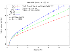
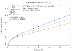
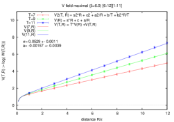
Figure 1: Static potential as a function of $R$: Panels show static potentials for YM field (left), for restricted field in the minimal option (center) and for restriced field in the maximal option (right). Each panel shows plots of data for $N_{T}=7,9,11$ cases, and fitted functions $V(T,R)$.

Figure 3 shows the combined plot of potentials for $N_{T}=10.$ We obtain string tension in the fitting range $6\leq R\leq 11$ as

$$\sigma_{YM}=0.589\pm 0.036\text{, \ \ \ }\sigma_{\min}=0.492\pm 0.0018,\text{ \ }\sigma_{\max}=0.494\pm 0.0014\text{ \ .}$$ (15)

We have the good agreement in the string tension between both options.

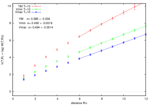
Figure 2: Comparison of static potentials:. the YM filed, the restricted field in the minimal and maximal options.

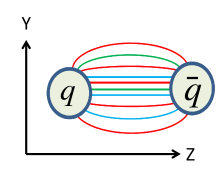
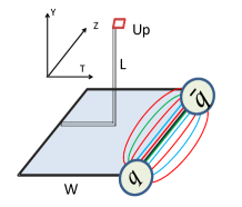
Figure 3: (Left) Set up of mesuarement of chromo flux. (Right) The gauge-invariant correlation operator $tr(WLU_{p}L^{\dagger})$ between a probe plaquatte $U_{p}$ and the source Wilson-loop $W$. .

3.2 Chromoelectric Flux

Next, we study the dual Meissner effect. For this purpose, we measure the chromo flux created by a quark-antiquark pair which is represented by the Wilson loop $W$ defined in the right panel of Figure 3. The chromo-field strength, i.e., the field strength of the chromo flux at the position $P$ is measured by using a plaquette variable $U_{p}$ as the probe operator for the field strength [16]:

$$\rho_{{}_{U_{P}}}:=\frac{\left\langle\mathrm{tr}\left(WLU_{p}L^{{\dagger}}\right)\right\rangle}{\left\langle\mathrm{tr}\left(W\right)\right\rangle}-\frac{1}{N_{c}}\frac{\left\langle\mathrm{tr}\left(U_{p}\right)\mathrm{tr}\left(W\right)\right\rangle}{\left\langle\mathrm{tr}\left(W\right)\right\rangle},$$ (16)

where $L$ is the Wilson line connecting the source $W$ and the probe $U_{p}$ needed to obtain the gauge-invariant result. Note that $\rho_{{}_{U_{P}}}$ is sensitive to the field strength rather than the disconnected one. To discriminate the chromo flux for each option, for the same source represented by the Wilson-loop made of the YM field we investigate the chromo flux by changing probe operators, $LU_{p}L^{{\dagger}},$made of the restricted fields in the minimal and maximal options in place of the original YM field.

Figure 4 shows the result of the measurement of chromo field strength for the original YM field, restricted field of the minimal and maximal options from left to right panels, respectively. We find that only the chromoelectric-flux tube is created between a quark and an anti-quark for both options.

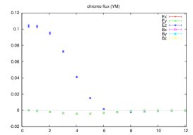
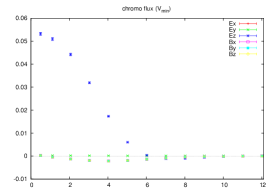
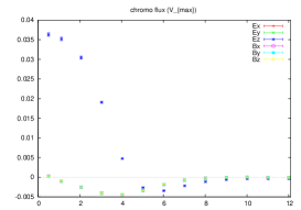
Figure 4: Measurment of the componet of the chromo flux. (Left) original YM field, (Center) ninimal option (Right) maximal option.

Finally, we investigate the dual Meissner effect by measuring the magnetic–monopole current $k$ induced around the chromoelectric-flux tube created by the quark-antiquark pair. We use the magnetic-monopole current $k$ defined by

$$k_{\mu}(x)=\frac{1}{2}\epsilon_{\mu\nu\alpha\beta}\left(F[V]_{\alpha\beta}(x+\hat{\nu})-F[V]_{\alpha\beta}(x)\right).$$ (17)

Note that the magnetic–monopole current (17) must vanish due to the Bianchi identity, if there exists no singularity in the gauge potential. Therefore, the magnetic–monopole current defined in this way can be the order parameter for the confinement/deconfinement phase transition, as suggested from the dual superconductivity hypothesis (see left panel of Figure 5). Center panel of Fig.5 shows the result of the measurements of the magnitude $\sqrt{k_{\mu}k_{\mu}}$ of the induced magnetic current $k_{\mu}$ obtained according to Eq.(17). Therefore, we find the dual Meissner effect in both options. Furthermore, in the maximal option we can decompose the magnetic-monople current into the two channels, $k_{\mu}(x)=$ $k_{\mu}^{(3)}(x)+k_{\mu}^{(8)}(x)$ which correspond to two types of color fields $\mathbf{n}_{x}^{(3)}$ and $\mathbf{n}_{x}^{(8),}$respectively. Right panel of Fig.5 shows the result of the decomposition. This shows that two types of magnetic monopole contribute to confinement in the same weight.

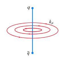
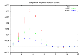
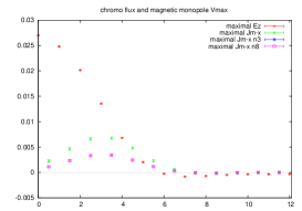
Figure 5: Measurement of the induced magnetic-monopole current. (Left) Sketch of induced magnetic monopole current around the chromoelectric flux tube. (Center) Measurement of the induced magetic monopole currents for YM-field (red), minimal option (green) and maximal option (blue). (Right) Anatomy of the induced magnetic-monopole current for the maximal option. The upper to lower plots represent respectively the chromoelectric field ($E_{Z})$ and the total induced magnetic-monopole current, and decomposed ones corresponding to the color field $n^{(3)}$ and $n^{(8)}$.

4 Summary and outlook

By using a new formulation of YM theory, we have investigated two possible types of the dual superconductivity picture in the $SU(3)$ YM theory, i.e., the non-Abelian dual superconductivity as the minimal option and the conventional Abelian dual superconductivity as the maximal option. In the measurement for both maximal and minimal options, we have found the linear static potential between a pair of quark and antiquark as for the original YM field and also the V-field dominance in the string tension for each option. The string tension for both options has almost the same value  We, then, have investigated the dual Meissner effect and found the chromoelectoric-flux tube in each option. We have also found the induced magnetic-monopole current due to the dual Meissner effect.

Acknowledgement

This work is supported by Grant-in-Aid for Scientific Research (C) 24540252 and 15K05042 from Japan Society for the Promotion Science (JSPS), and in part by JSPS Grant-in-Aid for Scientific Research (S) 22224003. The numerical calculations are supported by the Large Scale Simulation Program No.13/14-23 (2013-2014) and No.14/15-24 (2014-2015) of High Energy Accelerator Research Organization (KEK).

References

• [1] Kei-Ichi Kondo, Seikou Kato, Akihiro Shibata and Toru Shinohara, Phys.Rept. 579 (2015) 1-226, arXiv:1409.1599 [hep-th]
• [2] Y. Nambu, Phys. Rev. D10, 4262(1974); G. ’t Hooft, in High Energy Physics, edited by A. Zichichi (Editorice Compositori, Bologna, 1975); S. Mandelstam, Phys. Report 23, 245(1976); A.M. Polyakov, Nucl. Phys. B120, 429(1977).
• [3] K.-I. Kondo, T. Murakami and T. Shinohara, Eur. Phys. J. C 42, 475 (2005); K.-I. Kondo, T. Murakami and T. Shinohara, Prog. Theor. Phys. 115, 201 (2006).; K.-I. Kondo, T. Shinohara and T. Murakami, Prog.Theor. Phys. 120, 1 (2008)
• [4] K.-I. Kondo, A. Shibata, S. Kato, T. Shinohara, T. Murakami, Phys.Lett. B669 (2008) 107-118
• [5] K.-I. Kondo, A. Shibata, T. Shinohara, S. Kato, Phys.Rev. D83 (2011) 114016
• [6] A. Shibata, K.-I. Kondo, S. Kato and T. Shinohara, Phys.Rev. D87 (2013) 5, 05401
• [7] Akihiro Shibata, Kei-Ichi Kondo, Seikou Kato, Toru Shinohara, PoS LATTICE2013 (2014)
• [8] A. Shibata, K.-I. Kondo, S. Kato and T. Shinohara, PoS LATTICE2014 (2015) 340 KEK-PREPRINT-2014-43, CHIBA-EP-210
• [9] A. Shibata, K.-I. Kondo, S. Kato and T.Shinohara, KEK-PREPRINT-2015-49 CHIBA-EP-214
• [10] A. Shibata, K.-I. Kondo and T. Shinohara, Phys.Lett.B691:91-98 (2010)
• [11] Y.M. Cho, Phys. Rev. D 21, 1080 (1980). Phys. Rev. D 23, 245 (1981); Y.S. Duan and M.L. Ge, Sinica Sci., 11, 1072(1979); L. Faddeev and A.J. Niemi, Phys. Rev. Lett. 82, 1624 (1999); S.V. Shabanov, Phys. Lett. B 458, 322 (1999). Phys. Lett. B 463, 263 (1999).
• [12] A. Shibata, S. Kato, K.-I. Kondo, T. Shinohara  and S. Ito, POS(LATTICE2007) 331
• [13] Nigel Cundy, Y.M. Cho, Weonjong Lee, Jaehoon Leem, Phys.Lett. B729 192-198 (2014)
• [14] Shinya Gongyo, Takumi Iritani and Hideo Suganuma, Phys.Rev. D86 (2012) 094018
• [15] H. Suganuma and N. Sakumichi, Phys.Rev. D90 (2014) 11, 111501
• [16] A. Di Giacomo, M. Maggiore, and S. Olejnik, Phys. Lett. B236, 199 (1990); Nucl. Phys. B347, 441 (1990).