Direct state reconstruction with coupling-deformed pointer observables

Abstract

Direct state tomography (DST) using weak measurements has received wide attention. Based on the concept of coupling-deformed pointer observables presented by Zhang et al.[Phys. Rev. A 93, 032128 (2016)], a modified direct state tomography (MDST) is proposed, examined, and compared with other typical state tomography schemes. MDST has exact validity for measurements of any strength. We identify the strength needed to attain the highest efficiency level of MDST by using statistical theory. MDST is much more efficient than DST in the sense that far fewer samples are needed to reach DST’s level of reconstruction accuracy. Moreover, MDST has no inherent bias when compared to DST.

I Introduction

Though the quantum no-clone theorem prohibits the perfect estimation of the unknown state of a single quantum system ncl1 ; ncl2 , state reconstruction is possible via repeatedly measuring an ensemble of identical systems, a process usually called quantum state tomography (QST). Besides the standard QST strategies qst1 ; qst2 ; qst3 ; qst4 ; qst5 ; qst6 ; qst7 ; qst8 , a novel tomography strategy, conventionally called direct state tomography (DST), or weak-value tomography, has been widely investigated both theoretically and experimentally  dsm1 ; dsm2 ; dsm3 ; dsm4 ; dsm5 ; dsm7 ; dimension ; comwave ; high .

DST is based on the quantum weak value theory introduced by Aharonov, Albert and Vaidman (AAV) in 1988 aav . In DST, each element of the unknown density operator is proportional to a single weak value, if we choose the appropriate variables in weak measurements dsm3 . In this way, the wave function at each point can be determined directly, without the global inversion required in standard QST dsm7 . Because of this feature and the simplicity of experimental implementation, DST can be conveniently realized and is probably the only choice for the tomography of high-dimensional states dimension ; comwave ; high .

However, as pointed out in mac , DST suffers from the disadvantages, including low efficiency and systematical reconstruction bias. It is conceivable that these flaws mainly stem from the AAV’s weak-value formalism that built on first-order perturbation of the measurement strength wk1 ; wk2 ; wk3 ; wk4 . That is, very weak coupling strength causes the low efficiency of DST mac ; approximations produce unavoidable bias mac .

Recently, we have constructed a new framework for quantum measurements with postselection zhan . In our formalism, weak value information can be generated exactly with measurements of any strength, provided that two coupling-deformed(CD) pointer observables are read on the pointer of the quantum measuring device zhan . The general formula for determining the CD observables was also given in zhan . In particularly, when a single qubit is used as the measuring device, it is also reported in Refs. vall ; zou that weak values can be obtained from stronger measurements by standard state tomography of the qubit device.

In this paper, we propose a modified DST that works by applying the CD observables zhan in state tomography; it will be denoted as MDST hereafter. Since MDST is valid over the full range of measurement strength, we will determine the optimal measurement strength at which MDST attains its highest efficiency. Then, through Monte Carlo simulations, we demonstrate that the efficiency of MDST is much higher than that of DST. That is, to reach the same level of reconstruction accuracy, MDST needs far fewer samples. Furthermore, MDST is also compared with SU(2) tomography, one of the most efficient stand QST qst1 .

This paper is organized as follows. We briefly review SU(2) tomography and DST in Sec. II. In Sec. III, MDST is studied and the optimal coupling strength is given. In section IV, the performance of different state reconstruction strategies are compared using Monte Carlo simulation results. A short conclusion is presented in Sec. V.

II Strategies for quantum state reconstruction

In this section, we briefly review SU(2) tomography, and the original direct state tomography (DST).

II.1 SU(2) tomography

SU(2) tomography is a well-established state reconstruction technique. It is based on the formula qst1

$$\rho_{in}=\int dgR^{\dagger}\left(g\right)\mathrm{tr}[\rho_{in}R(g)],$$ (1)

where $R\left(g\right)$ is the unitary irreducible square-integrable representation of a tomographic group $G$, $g\in G$. The derivation of Eq. (1) can be found in qst1 . As indicated by Eq. (1), a general unknown state $\rho_{in}$ could be reconstructed by a series of projective measurements onto the eigenstates of $R(g)$. When the tomographic group $G$ is selected to be the SU(2) group, the tomography scheme is called SU(2) tomography (see  qst1 for the details).

Additionally, standard tomography can be implemented with measurements of the basis operators of the space of density matrices. For example, an unknown qubit state can be expressed using the Pauli matrices

$$\rho_{in}=\frac{I}{2}+\sum_{i=x,y,z}\sigma_{i}\;\mathrm{tr}(\rho_{in}\sigma_{i}).$$ (2)

By measuring the three Pauli matrices, we could reconstruct an unknown two-dimensional state.

II.2 Direct state tomography

The original direct state tomography (DST) is based on weak measurements. Suppose a system in unknown state $\rho_{in}$ is weakly measured by a pointer in state $|\phi_{0}\rangle$. The observables being measured on the system are chosen in the set $\{A_{i}=|a_{i}\rangle\langle a_{i}|\}_{i}$. Therein, states $\{|a_{i}\rangle\}_{i}$ compose an orthogonal basis of the system’s Hilbert space. After that measurement we project the system onto another orthogonal basis $\{|\psi_{f}\rangle\}_{f}$ of the system’s Hilbert space, a process conventionally called postselection ( In this article, postselection represents the final projective measurement, and no data is discarded in the state reconstruction process.). We then record the outcome of the postselection, read the pointer by the pointer observable denoted as $\hat{s}$, and generate the the weak value of each $A_{i}$ defined as dsm3

$$W_{if}=\frac{\langle\psi_{f}|a_{i}\rangle\langle a_{i}|\rho_{in}|\psi_{f}\rangle}{P_{f}},$$ (3)

where $P_{f}$ is the probability of obtaining $|\psi_{f}\rangle$ in postselection. For convenience, the measurement basis $\{|a_{i}\rangle\}_{i}$ and the postselection basis $\{|\psi_{f}\rangle\}_{f}$ are chosen to be the mutually unbiased bases (MUB) that $|\langle\psi_{f}|a_{i}\rangle|=1/\sqrt{d}$ mub . Using the weak values $\{W_{if}\}_{i,f}$, we can reconstruct the unknown state using the formula

$$\rho_{r}=\sum_{i,f=1}^{d}\frac{P_{f}W_{if}}{\langle\psi_{f}|a_{i}\rangle}|a_{i}\rangle\langle\psi_{f}|.$$ (4)

This formula states that no samples are discarded, which is different with the original pure-state tomography case in Ref. [11]. In the direct state tomography strategy of this article, each sample is used to construct weak values $\{W_{if}\}_{i,f}$ no matter which of $\{|\psi_{f}\rangle\}_{f}$ is obtained in postselection.

In this paper, we consider the setup of dsm1 where the pointer is a qubit initialized in pure state $\rho_{\phi}=|0\rangle\langle 0|$, the eigenstate of $\sigma_{z}$: $\sigma_{z}|0\rangle=|0\rangle$. The weak measurement is described by the unitary coupling

$$U_{i}(g)=\exp(-igA_{i}\otimes\sigma_{x}),$$ (5)

where the coupling strength $g$ is small. The weak value is determined via measuring two different observables on the pointer, i.e., $\hat{s}\in\{\hat{q},\hat{p}\}$, $\hat{q}$ for the real part and $\hat{p}$ for the imaginary part. They could be

$$\hat{q}=\sigma_{y},\qquad\hat{p}=\sigma_{x}.$$ (6)

The weak value is determined by

$$P_{f}W_{if}=\lim_{g\rightarrow 0}\frac{1}{2g}\mathrm{tr}\{U_{i}(g)\rho_{in}\otimes\rho_{\phi}U_{i}^{\dagger}(g)\Pi_{f}\otimes(-\hat{q}+i\hat{p})\},$$ (7)

where $\Pi_{f}=|\psi_{f}\rangle\langle\psi_{f}|$. That is, the weak value information is obtained by measuring $\Pi_{f}\otimes\hat{s}$ on the joint system.

The validity of Eq. (7) requires $g\rightarrow 0$, which implies little information gain zhu and low efficiency for DST. However, $g$ is small but finite in an actual experiment, thus a systematical error in the reconstruction is unavoidable. These two disadvantages of DST have been verified by numerical simulations in mac .

III Modified direct state tomography

A recent work shows that weak value can be obtained exactly with measurements of any strength, if we measure the coupling-deformed (CD) pointer observables given inzhan . In this section, we will use this strategy to propose a modified direct state tomography (MDST), and identify the optimal coupling strength which maximizes the efficiency of MDST.

III.1 MDST with CD pointer observables

When $g\to 0$, we measure the observable $\hat{s}\in{\hat{p},\hat{q}}$ given by Eq. (6) on the pointer to get weak value information. In Ref. zhan , we can obtain the exact weak value information by measuring the CD observable $\hat{s}(g)$ that varies with $g$, instead of $\hat{s}$. For the two observables $\hat{p}$ and $\hat{q}$ in Eq. 6, using the method in zhan , the corresponding CD pointer observables $\hat{q}(g)$ and $\hat{p}(g)$ are calculated to be

$$\hat{q}(g)=\frac{1}{\sin g}\left(\sigma_{y}-\tan(\frac{g}{2})(I-\sigma_{z})\right);$$ (8)

$$\hat{p}(g)=\frac{1}{\sin g}\sigma_{x}.$$

Then the weak value information is exactly obtained via

$$P_{f}W_{if}=\frac{1}{2}\mathrm{tr}\{U_{i}(g)\rho_{in}\otimes\rho_{\phi}U_{i}^{\dagger}(g)\Pi_{f}\otimes[-\hat{q}(g)+i\hat{p}(g)]\}.$$ (9)

With the set $\{P_{f}W_{if}\}_{(i,f)}$, $\rho_{in}$ can be reconstructed via Eq. (4). We call this scheme modified direct state tomography (MDST).

By comparing Eq. (7) and Eq. (9), it is straightforward to see that in MDST, no approximation is applied, thus there will be no inherent bias in the reconstruction, and MDST can be implemented with any value of $g$.

Here, we would like to remark that our presentation of DST and MDST is slightly different from others focusing on AAV’s weak value, for example dsm7 . If using the whole weak value, there will be an unknown normalization factor that can be fixed only after all the measurements are completed vall . This is seen as conflicting with the claim of directness gro . However, in our MDST, Eq. (4) clearly shows that one element is directly determined by $P_{f}W_{if}$, which could be obtained from the measurements described in Eq. (9).

III.2 The optimal measurement strength in MDST

Since in MDST $g$ can be any value, we need to search for the optimal strength to obtain the highest efficiency. First, we derive the optimal $g$ by statistical theory. In actual implementation, MDST suffers from statistical errors. This is the reason why there is a discrepancy between the true state $\rho_{t}$ and the reconstructed state $\rho_{r}$. Statistical errors can be quantified by the variance of the measured results. Lower variance means less random error and higher reconstruction accuracy. We find that when gauging the performance of MDST by the variance of the reconstruction, the optimal value of $g$ will be appealingly state-independent.

From Eq. (4), each element of the reconstruction $\rho_{r}$

$$\varrho_{if}={P_{f}W_{if}}/{\langle\psi_{f}|a_{i}\rangle}$$ (10)

is determined by two independent measurements, one for the real part and the other for the imaginary part of $\varrho_{if}$. Therefore, the total variance of the reconstruction state $\rho_{r}$ can be defined as

$$\delta^{2}\rho_{r}=\sum_{i,f=1}^{d}\delta^{2}(\Re\varrho_{if})+\delta^{2}(\Im\varrho_{if}),$$ (11)

where $\Re$ and $\Im$ stand for the real and imaginary part, respectively. From Eqs. (4) and (9), the convention $|\langle\psi_{f}|a_{i}\rangle|=1/\sqrt{d}$, and the error propagation theory error , the total variance $\delta^{2}\rho_{r}$ can be expressed as

$$\delta^{2}\rho_{r}=\frac{d}{4} \sum_{\hat{s}\in\{\hat{q},\hat{p}\}}\sum_{i,f=1}^{d}\mathrm{tr}\{U_{i}\rho_{t}\otimes\rho_{\phi}U_{i}^{\dagger}\Pi_{f}\otimes\hat{s}^{2}(g)\}$$ (12)

$$-\left(\mathrm{tr}\{U_{i}\rho_{t}\otimes\rho_{\phi}U_{i}^{\dagger}\Pi_{f}\otimes\hat{s}(g)\}\right)^{2},$$

As shown in Eq. (9), the second term in the summation gives the squares of the real or imaginary parts of $\varrho_{if}$. Since it is independent of $g$, we only need to focus on the summation of the first term of Eq. (12), which will be denoted as $TV1$. Using the relation that $\sum_{f}\Pi_{f}=I_{s}$ (the identity on the system’s Hilbert space), we have

$$TV1=\frac{d}{4}\sum_{\hat{s}\in\{\hat{p},\hat{q}\}}\sum_{i=1}^{d}\mathrm{tr}\{\rho_{i}\hat{s}^{2}(g)\}$$ (13)

where $\rho_{i}=\mathrm{tr}_{s}(U_{i}\rho_{t}\otimes\rho_{\phi}U_{i}^{\dagger})$. Since $\hat{p}(g)^{2}=1/\sin^{2}(g)$, we obtain

$$\mathrm{tr}\{\rho_{i}\hat{p}^{2}(g)\}=\frac{1}{\sin^{2}(g)},$$ (14)

which is independent on the input state $\rho_{t}$. For $\hat{s}(g)=\hat{q}(g)$, we have

$$\mathrm{tr}_{a} \{\rho_{i}\hat{q}^{2}(g)\}=\frac{1}{\sin^{2}g}+\frac{2c_{i}}{\cos^{2}\frac{g}{2}},$$ (15)

where $c_{i}=\langle a_{i}|\rho_{t}|a_{i}\rangle$. Since $\sum_{i}c_{i}=1$, TV1 is evaluated as

$$TV1=\frac{d^{2}}{2\sin^{2}g}+\frac{d}{2\cos^{2}\frac{g}{2}},$$ (16)

where $d$ is the dimension of the unknown state. TV1, and thus $\delta^{2}\rho_{r}$, attains the minimum at the optimal strength

$$g_{opt}=\arccos(1+\frac{d}{2}-\sqrt{d+\frac{d^{2}}{4}}).$$ (17)

In Fig. 1, the value of TV1 against the coupling strength $g\in[1,1.6]$ is illustrated for the two-dimensional systems. From Eq. (17), the minimum of $TV1$ locates at $g=1.30$. It may be surprising at first glance that $g=\pi/2$, which makes the coupling unitary Eq. (5) describe the strongest measurement, is not optimal. Our result $g_{opt}=1.3$ is also consistent with the result of $g_{opt}\approx 1.25$ gro , which is calculated using the average fidelity as the figure of merit of the reconstruction of the pure qubit states in the scheme introduced by Vallone and Dequal vall .

In order to align with the results in mac , we will use the trace distance to quantify the accuracy of the reconstruction. To locate the optimal strength with respect to trace distance, we use the standard Monte Carlo method to simulate MDST: first, a two-dimensional mixed state $\rho_{t}$ is selected randomly as the target state; second, the reconstruction $\rho_{r}$ is produced by MDST with $10^{3}$ copies of $\rho_{t}$ for different coupling strengths; third, the trace distance niel between $\rho_{t}$ and $\rho_{r}$,

$$D(\rho_{t},\rho_{r})=\frac{\mathrm{tr}\left(|\rho_{t}-\rho_{r}|\right)}{2},$$ (18)

is calculated to gauge the performance of MDST. Smaller trace distance $D(\rho_{t},\rho_{r})$ means higher efficiency. In order to eliminate statistical fluctuations, we have averaged $D(\rho_{t},\rho_{r})$ over $10^{5}$ randomly selected $\rho_{t}$. The simulation results are presented in Fig. 1. It coincides well with the prediction of variance that $g_{opt}=1.3$.

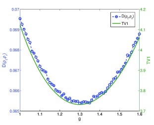
Figure 1: (Color online) The values of TV1 (green line) of the reconstruction, and trace distance $D(\rho_{t},\rho_{r})$ (blue circles) averaged over $10^{5}$ states, against the coupling strength.

IV Comparison

The value of TV1 diverges at the weak limit $g\rightarrow 0$. This demonstrates the conclusion that DST at the weak limit suffers serious random noise, which leads to low efficiency. The exactness of the MDST formalism, and its validity over the entire range of measurement strength suggest that MDST can overcome the problems of low efficiency and intrinsic bias. In this section, we will examine this claim by using Monte Carlo simulations to compute the three strategies of quantum state reconstruction: MDST, DST, and SU(2) tomography.

The simulation goes as follows. First, a state is reconstructed by MDST, DST, Pauli tomography and SU(2) tomography; second, the trace distance $D(\rho_{t},\rho_{r})$ between the true state $\rho_{t}$ and the reconstructed state $\rho_{r}$ is used to gauge the estimation efficiency. Given equivalent sample size, the smaller the trace distance is, the higher the efficiency of a tomography scheme will be.

As shown in Fig. 2, all the reconstruction strategies are affected by statistical errors. The trace distances decrease with the the numbers of the copies of the systems. As expected from the simulation results, the reconstruction $\rho_{r}$ of DST has a systematical bias, while the state $\rho_{r}$ obtained by MDST has no error bias. The trace distance $D(\rho_{t},\rho_{r})$ continues to decrease as the number of copies increases.

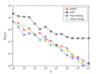
Figure 2: (Color online) Comparison of the efficiencies of MDST, DST, SU(2) tomography and Pauli tomography for qubits. The trace distance $D(\rho_{t},\rho_{r})$ is plotted as the function of the number of copies N of the system. Circles, D calculated from MDST with $g=1.3$; squares, D calculated from DST with $g=0.1$; diamonds, D calculated from Pauli tomography; stars, D calculated from SU(2) tomography.

For quibts, as indicated in Fig. 2, the efficiencies of MDST, Pauli tomography and SU(2) tomography differ little. For five-dimensional systems, as shown in Fig. 3, the relationship between the trace distance and the number of copies is given. These two figures clearly show that to reach the same level of trace distance, MDST uses far fewer samples than DST. That is to say, the efficiency of DST is significantly improved by using stronger measurements and CD pointer observables.

Figure 3 also indicates that MDST is less efficient than SU(2) tomography. For the same reconstruction precision, MDST needs more copies than SU(2) tomography. This is consistent with the result found in Ref. gro that the scheme of Haar-uniform randomly chosen one-dimensional orthogonal projective measurements is more efficient than direct tomography methods.

In order to study the gap between the efficiencies of MDST and SU(2) tomography, we have performed further simulations for two, four, five, six, eight, nine, and ten-dimensional systems. In the tables of the appendix, we list the reconstruction precision gauged by trace distance, and the corresponding samples size $N_{MDST}$ and $N_{SU(2)}$, which are averaged over 500 repeated reconstructions to decrease the statistical fluctuation.

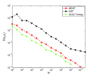
Figure 3: (Color online) Comparison of MDST, DST and SU(2) tomography for five-dimensional states. The trace distance $D(\rho_{t},\rho_{r})$ is plotted as the function of the number of copies N of the system. Circles, D calculated from MDST with $g=1.4$; squares, D calculated from DST with $g=0.1$; stars, D calculated from SU(2) tomography.

As indicated in Tables I-III, for the expected trace distances $D$, the results suggest that $N_{MDST}\approx 0.8dN_{SU(2)}$ for two, four and five-dimensional systems, where $d$ is the dimension of the systems. In Tables IV-V, for six and eight-dimensional states, it is shown that $N_{MDST}\approx 0.75dN_{SU(2)}$. In Tables VI-VII, $0.7dN_{SU(2)}$ copies are needed in MDST to attain the same precision of SU(2) tomography for nine and ten-dimensional systems. Roughly speaking, we suppose $N_{MDST}\approx 0.8dN_{SU(2)}$.

From the data obtained in simulations, we estimate that to reach an equivalent level of reconstruction accuracy, the sample size required in MDST, $N_{MDST}$, is about $0.8d$ times of $N_{SU(2)}$, the sample size required in SU(2) tomography. MDST is clearly less efficient than SU(2) tomography, especially for high dimensional systems.

Since SU(2) tomography is predicted on measuring a complete set of non-commuting observables, a difficult task to realize in actual experiments. Although MDST is less efficient than SU(2) tomography, MDST is much easier to implement in experiments. MDST might be more useful than SU(2) tomography for reconstructing an unknown state, especially for high dimensional states.

V conclusion

In this paper, we have presented a modified direct state tomography (MDST) using the coupling-deformed pointer observables. We have verified that MDST has no inherent bias. MDST is valid for any large coupling strength. We have obtained the optimal measurement strength with which the efficiency of MDST is much higher than that of DST. Numerical simulation also suggests that the efficiency of MDST is less than SU(2) tomography. However, MDST is much easier to implement in actual experiments, and it thus could be useful in reconstructing unknown quantum states.

Appendix

In this appendix, we list seven tables to present the state reconstruction precision levels and the numbers needed in MDST and SU(2) tomography respectively. All the trace distances are averaged over $10^{3}$ repeated reconstructions to eliminate statistical fluctuations.

MDST $g=1.3$	$N_{1}=1600$	$N_{2}=2560$	$N_{3}=4096$
	$D_{1}=0.0497$	$D_{2}=0.0386$	$D_{3}=0.0300$
SU(2) tomography	$N_{1}^{\prime}=1000$	$N_{2}^{\prime}=1600$	$N_{3}^{\prime}=2560$
	$D_{1}^{\prime}=0.0499$	$D_{2}^{\prime}=0.0384$	$D_{3}^{\prime}=0.0299$

Table 1: The trace distances $D$ ($D^{\prime}$) and the number $N$ ($N^{\prime}$) of copies needed for two-dimensional systems in MDST (SU(2) tomography).

MDST $g=1.4$	$N_{1}=3200$	$N_{2}=10240$	$N_{3}=32768$
	$D_{1}=0.140$	$D_{2}=0.0780$	$D_{3}=0.0435$
SU(2) tomography	$N_{1}^{\prime}=1000$	$N_{2}^{\prime}=3200$	$N_{3}^{\prime}=10240$
	$D_{1}^{\prime}=0.141$	$D_{2}^{\prime}=0.0784$	$D_{3}^{\prime}=0.0435$

Table 2: The trace distances $D$ ($D^{\prime}$) and the number $N$ ($N^{\prime}$) of copies needed for four-dimensional systems in MDST (SU(2) tomography).

MDST $g=1.4$	$N_{1}=4000$	$N_{2}=16000$	$N_{3}=64000$
	$D_{1}=0.192$	$D_{2}=0.0961$	$D_{3}=0.0481$
SU(2) tomography	$N_{1}^{\prime}=1000$	$N_{2}^{\prime}=4000$	$N_{3}^{\prime}=16000$
	$D_{1}^{\prime}=0.196$	$D_{2}^{\prime}=0.0977$	$D_{3}^{\prime}=0.0482$

Table 3: The trace distances $D$ ($D^{\prime}$) and the number $N$ ($N^{\prime}$) of copies needed for five-dimensional systems in MDST (SU(2) tomography).

MDST $g=1.4$	$N_{1}=9000$	$N_{2}=40500$	$N_{3}=182250$
	$D_{1}=0.182$	$D_{2}=0.0849$	$D_{3}=0.0404$
SU(2) tomography	$N_{1}^{\prime}=2000$	$N_{2}^{\prime}=9000$	$N_{3}^{\prime}=40500$
	$D_{1}^{\prime}=0.184$	$D_{2}^{\prime}=0.0864$	$D_{3}^{\prime}=0.0409$

Table 4: The trace distances $D$ ($D^{\prime}$) and the number $N$ ($N^{\prime}$) of copies needed for six-dimensional systems in MDST (SU(2) tomography).

MDST $g=1.4$	$N_{1}=18000$	$N_{2}=108000$	$N_{3}=648000$
	$D_{1}=0.224$	$D_{2}=0.0916$	$D_{3}=0.0374$
SU(2) tomography	$N_{1}^{\prime}=3000$	$N_{2}^{\prime}=18000$	$N_{3}^{\prime}=108000$
	$D_{1}^{\prime}=0.233$	$D_{2}^{\prime}=0.0954$	$D_{3}^{\prime}=0.0390$

Table 5: The trace distances $D$ ($D^{\prime}$) and the number $N$ ($N^{\prime}$) of copies needed for eight-dimensional systems in MDST (SU(2) tomography).

MDST $g=1.4$	$N_{1}=31500$	$N_{2}=94500$	$N_{3}=315000$
	$D_{1}=0.211$	$D_{2}=0.123$	$D_{3}=0.0677$
SU(2) tomography	$N_{1}^{\prime}=5000$	$N_{2}^{\prime}=15000$	$N_{3}^{\prime}=50000$
	$D_{1}^{\prime}=0.214$	$D_{2}^{\prime}=0.126$	$D_{3}^{\prime}=0.0683$

Table 6: The trace distances $D$ ($D^{\prime}$) and the number $N$ ($N^{\prime}$) of copies needed for nine-dimensional systems in MDST (SU(2) tomography).

MDST $g=1.4$	$N_{1}=21000$	$N_{2}=70000$	$N_{3}=210000$
	$D_{1}=0.316$	$D_{2}=0175$	$D_{3}=0.100$
SU(2) tomography	$N_{1}^{\prime}=3000$	$N_{2}^{\prime}=10000$	$N_{3}^{\prime}=30000$
	$D_{1}^{\prime}=0.327$	$D_{2}^{\prime}=0.180$	$D_{3}^{\prime}=0.103$

Table 7: The trace distances $D$ ($D^{\prime}$) and the number $N$ ($N^{\prime}$) of copies needed for ten-dimensional systems in MDST (SU(2) tomography).

References

- (1) W. K. Wootters, W. H. Zurek, Nature (London) 299, 802(1982).
- (2) G. M. D’Ariano and H. P. Yuen, Phys. Rev. Lett. 76, 2832 (1996).
- (3) G. M. D’Ariano, L. Maccone, and M. Paini, J. OPT. B: Quantum Semicalss. Opt. 5, 77 (2003).
- (4) G. M. D’Ariano, L. Maccone, and M. G. A. Paris, J. Phys. A 34, 93 (2001).
- (5) D. F. V. James, P. G. Kwiat, W. J. Munro, and A. G. White, Phys. Rev. A 64, 052312 (2001).
- (6) A. E. Allahverdyan, R. Balian, and Th. M. Nieuwenhuizen, Phys. Rev. Lett. 92, 120402 (2004).
- (7) G. M. D’Ariano, L. Maccone, and M. F. Sacchi, in Qautnum information with Continuous Variables of Atoms and Light, edited by N.Cerf, G. Leuchs, and E. Polzik (World Scientific Press, London, 2007).
- (8) T. Durt, C. Kurtsiefer, A. Lamas-Linares, and A. Ling, Phys. Rev. A 78, 042338 (2008).
- (9) R. B. A. Adamson and A. M. Steinberg, Phys. Rev. Lett. 105, 030406 (2010).
- (10) H. Wang, W. Zheng, Y. Yu, M. Jiang, X. Peng, and J. Du, Phys. Rev. A 89, 032103 (2014).
- (11) J. S. Lundeen, B. Sutherland, A. Patel, C. Stewart, and C. Bamber, Nature (London) 474, 188 (2011).
- (12) H. F. Hofmann, Phys.Rev. A 81, 012103 (2010).
- (13) S. Wu, Sci. Rep. 3, 1193 (2013).
- (14) J. Z. Salvail, M. Agnew, A. S. Johnson, E. Bolduc, J. Leach, and R. W. Boyd, Nat. Photon. 7, 316 (2013).
- (15) Y. Shikano, in Measurements in Quantum Mechanics, edited by M. R. Pahlavani (InTech, Rijeka, 2012), p. 75.
- (16) J. S. Lundeen and C. Bamber, Phys. Rev. Lett. 108, 070402 (2012).
- (17) M. Malik, M. Mirhosseini1, M. P. J. Lavery, J. Leach, M. J. Padgett, and R. W. Boyd, Nature Commun. 5, 3115 (2014)
- (18) M. Mirhosseini, O. S. Magaña-Loaiza, S. M. Hashemi Rafsanjani, and R. W. Boyd, Phys. Rev. Lett. 113, 090402 (2014).
- (19) Z. Shi, M. Mirhosseini, J. Margiewicz, M. Malik, F. Rivera, Z. Zhu, and R. W. Boyd, Optica 2, 388 (2015).
- (20) Y. Aharonov, D. Z. Albert, and L. Vaidman, Phys. Rev. Lett. 60 (1988) 1351.
- (21) L. Maccone and C. C. Rusconi, Phys. Rev. A 89, 022122 (2014).
- (22) I. M. Duck, P. M. Stevenson, and E. C. G. Sudarshan, Phys. Rev. D 40, 2112 (1989).
- (23) R. Jozsa,Phys. Rev. A 76, 044103 (2007).
- (24) S. Wu and Y. Li, Phys. Rev. A 83, 052106 (2011).
- (25) X. Zhu, Y. Zhang, S. Pang, C. Qiao, Q. Liu, and S. Wu, Phys. Rev. A 84, 052111 (2011).
- (26) Y-X. Zhang, S. Wu, and Z-B. Chen, Phys. Rev. A 93, 032128 (2016).
- (27) G. Vallone and D. Dequal, Phys. Rev. Lett. 116, 040502 (2016).
- (28) P. Zou, Z-M. Zhang, and W. Song, Phys. Rev. A 91, 052109 (2015).
- (29) T. Durt, B. Englert, I. Bengtsson, and K. Zyczkowski, Int. J. Quantum Inf. 8, 535 (2010).
- (30) X. Zhu, Y. Zhang, Q. Liu, and S. Wu, Phys. Rev. A 85, 042330 (2012).
- (31) J. A. Gross, N. Dangniam, C. Ferrie, and C. M. Caves, Phys. Rev. A 92 062133 (2015).
- (32) I. G. Hughes and T. P. A. Hase, inMeasurements and Their Uncertainties: A Practical Guide to Modern Error Analysis, (Oxford University Press, New York, 2010), p. 38.
- (33) M. A. Nielsen, I. Chuang, in Quantum Computation and Quantum Information, (Cambridge University Press, Cambridge, 2000), p. 403.