An estimate of the hadronic vacuum polarization disconnected contribution to the anomalous magnetic moment of the muon from lattice QCD

Abstract

The quark-line disconnected diagram is a potentially important ingredient in lattice QCD calculations of the hadronic vacuum polarization contribution to the anomalous magnetic moment of the muon. It is also a notoriously difficult one to evaluate. Here, for the first time, we give an estimate of this contribution based on lattice QCD results that have a statistically significant signal, albeit at one value of the lattice spacing and an unphysically heavy value of the $u/d$ quark mass. We use HPQCD’s method of determining the anomalous magnetic moment by reconstructing the Adler function from time-moments of the current-current correlator at zero spatial momentum. Our results lead to a total (including $u$, $d$ and $s$ quarks) quark-line disconnected contribution to $a_{\mu}$ of $-0.15\%$ of the $u/d$ hadronic vacuum polarization contribution with an uncertainty which is 1% of that contribution.

I Introduction

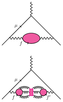
Figure 1: The hadronic vacuum polarization contribution to the muon anomalous magnetic moment is represented as a shaded blob inserted into the photon propagator (represented by a wavy line) that corrects the point-like photon-muon coupling at the top of each diagram. The top diagram is the connected contribution and the lower diagram the quark-line disconnected (but connected by gluons denoted by curly lines) contribution that is discussed here. The shaded box in the lower diagram indicates strong interaction effects that could occur between the two quark loops.

The high accuracy with which the magnetic moment of the muon can be determined in experiment makes it a very useful quantity in the search for new physics beyond the Standard Model. Its anomaly, defined as the fractional difference of its gyromagnetic ratio from the naive value of 2 ($a_{\mu}=(g-2)/2$) is known to 0.5 ppm Bennett et al. (2006). The anomaly arises from muon interactions with a cloud of virtual particles and can therefore probe the existence of particles that have not been seen directly. The theoretical calculation of $a_{\mu}$ in the Standard Model shows a discrepancy with the experimental result of about $25(8)\times 10^{-10}$ Aoyama et al. (2012); Hagiwara et al. (2011); Davier et al. (2011) which could be an exciting indication of new physics. Improvements by a factor of 4 in the experimental uncertainty are expected and improvements in the theoretical determination would make the discrepancy (if it remains) really compelling Blum et al. (2013).

The current theoretical uncertainty is dominated by that from the lowest order ($\alpha^{2}_{\mathrm{QED}}$) hadronic vacuum polarization (HVP) contribution, in which the virtual particles are strongly interacting, depicted in Fig. 1. This contribution, which we denote $a_{\mu,\mathrm{HVP}}$, is currently determined most accurately from experimental results on $e^{+}e^{-}\rightarrow$ hadrons or from $\tau$ decay to be of order $700\times 10^{-10}$ with a 1% uncertainty or better Hagiwara et al. (2011); Davier et al. (2011); Benayoun et al. (2015). This method for determining $a_{\mu,\mathrm{HVP}}$ does not distinguish the two diagrams of Fig. 1 because it uses experimental cross-section information, effectively including all possibilities for final states that would be seen if the two diagrams were cut in half.

$a_{\mu,\mathrm{HVP}}$ can also be determined from lattice QCD calculations using a determination of the vacuum polarization function at Euclidean-$q^{2}$ values Blum (2003). It is important that this is done to at least a comparable level of uncertainty to that obtained from the experimental results to provide a first-principles constraint of the values above. It is hoped that such calculations will, in time, allow the theoretical uncertainty to be reduced further.

Huge progress has been made in lattice QCD calculations in the last few years so that accuracies of a few percent in $a_{\mu,\mathrm{HVP}}$ are now achievable Burger et al. (2014). Indeed, a 1% determination of the $s$-quark contribution has been demonstrated Chakraborty et al. (2014). These calculations currently include only the quark-line connected contribution to the HVP, from the top diagram of Fig. 1. The quark-line disconnected contribution, from the lower diagram of Fig. 1, vanishes in the SU(3) limit but could still contribute several percent to $a_{\mu,\mathrm{HVP}}$ at physical $u$, $d$, and $s$ quark masses. It cannot therefore be left undetermined if 1% accuracy in $a_{\mu,\mathrm{HVP}}$ is to be achieved from lattice QCD calculations.

Quark-line disconnected diagrams are notoriously difficult to evaluate in lattice QCD because of poor signal-to-noise properties. Calculations of the disconnected contribution to $a_{\mu,\mathrm{HVP}}$ have concentrated on stochastic determinations using various noise-reduction methods and several calculations are underway, see, for example Ref. Guelpers et al. (2014).

Here we use instead lattice QCD results from the Hadron Spectrum Collaboration’s programme of calculations using distillation Peardon et al. (2009); Dudek et al. (2013a) in the light quark sector. These have enabled a clear signal to be obtained for quark-line disconnected correlators. Instead of using stochastic methods they rely on computing the correlator directly using sources made from a basis of vectors spanning the space of the smoothest quark fields. We combine this approach with HPQCD’s method of determining $a_{\mu,\mathrm{HVP}}$ by reconstructing the polarization function from its $q^{2}$-derivatives obtained from time-moments of correlators at zero spatial momentum Chakraborty et al. (2014). HPQCD’s approach enables existing meson correlators generated for determination of the spectrum, such as those of the Hadron Spectrum Collaboration, to be re-used for the determination of $a_{\mu,\mathrm{HVP}}$. Since the quark-line disconnected vector current correlator has been determined using distillation we normalise with the $\rho$ meson correlation function using the same method.

In Section II we give details of the method for determining $a_{\mu,\mathrm{HVP}}$ from lattice QCD correlators. This method leads to a simple (over)-estimate of the disconnected contribution using the physical properties of the $\rho$ and $\omega$ mesons given in Section III. In Section IV, we give the more complete results obtained from the Hadron Spectrum correlators. In Section V we discuss sources of systematic uncertainty in the results that lead finally in Section VI to a robust estimate of the impact of the disconnected contribution to $a_{\mu,\mathrm{HVP}}$ at the physical point.

II Determining $a_{\mu,\mathrm{HVP}}$ from current-current correlators

The contribution to the muon anomalous magnetic moment from the HVP is obtained by inserting the quark vacuum polarization into the photon propagator Blum (2003); Lautrup et al. (1972):

$$a_{\mu,\mathrm{HVP}}^{(\mathrm{f}\mathrm{f}^{\prime})}=\frac{\alpha}{\pi}\int_{0}^{\infty}dq^{2}f(q^{2})(4\pi\alpha Q_{\mathrm{f}}Q_{\mathrm{f}^{\prime}})\hat{\Pi}_{\mathrm{f}\mathrm{f}^{\prime}}(q^{2}),$$ (1)

where $\mathrm{f}$ and $\mathrm{f}^{\prime}$ refer to the quark flavours at the two ends of the polarization function. These two flavours need not be the same when we include the quark-line disconnected contribution from the lower diagram of Fig. 1. Here $\alpha\equiv\alpha_{\mathrm{QED}}$ and $Q_{\mathrm{f}}$ is the electric charge of quark $\mathrm{f}$ in units of $e$. The function $f(q^{2})$ is given by

$$f(q^{2})\equiv\frac{m_{\mu}^{2}q^{2}A^{3}(1-q^{2}A)}{1+m_{\mu}^{2}q^{2}A^{2}}$$ (2)

where

$$A\equiv\frac{\sqrt{q^{4}+4m_{\mu}^{2}q^{2}}-q^{2}}{2m_{\mu}^{2}q^{2}}.$$ (3)

The behaviour of $f(q^{2})$ means that the integral of eq. (1) is dominated by small values of $q^{2}$ ($\approx m^{2}_{\mu}$) and hence it is the behaviour of $\hat{\Pi}$ at values of $q^{2}$ close to zero that needs to be determined in lattice QCD.

The quark polarization tensor is the Fourier transform of the vector current-current correlator. For spatial currents at zero spatial momentum

$$\Pi^{ii}_{\mathrm{f}\mathrm{f}^{\prime}}(q^{2})=q^{2}{\Pi}_{\mathrm{f}\mathrm{f}^{\prime}}(q^{2})=a^{4}\sum_{t}e^{iqt}\sum_{\vec{x}}\langle j^{i}_{\mathrm{f}}(\vec{x},t)j^{i}_{\mathrm{f}^{\prime}}(0)\rangle$$ (4)

with $q$ the Euclidean energy. We need the renormalized vacuum polarization function, $\hat{\Pi}(q^{2})\equiv\Pi(q^{2})-\Pi(0)$, which automatically removes non-zero contributions to $\Pi(0)$ from non-conserved vector currents. Time-moments of the correlator give the derivatives at $q^{2}=0$ of $\hat{\Pi}$ (see, for example, Allison et al. (2008); McNeile et al. (2010)):

$$G_{2n,\mathrm{f}\mathrm{f}^{\prime}} \equiv a^{4}\sum_{t}\sum_{\vec{x}}t^{2n}Z_{V}^{2}\langle j^{i}_{\mathrm{f}}(\vec{x},t)j^{i}_{\mathrm{f}^{\prime}}(0)\rangle$$ (5)

$$= (-1)^{n}\left.\frac{\partial^{2n}}{\partial q^{2n}}q^{2}\hat{\Pi}_{\mathrm{f}\mathrm{f}^{\prime}}(q^{2})\right|_{q^{2}=0}.$$

Here we have allowed for a renormalization factor $Z_{V}$ for the lattice vector current. Note that time-moments remove any contact terms between the two currents. $G_{2n}$ is easily calculated from lattice QCD correlators, remembering that $t$ is zero at the origin and takes positive values in the positive time direction (up to $T/2-1$) and negative values in the negative time direction (down to $-T/2+1$).

Defining

$$\hat{\Pi}(q^{2})=\sum_{j=1}^{\infty}q^{2j}\Pi_{j}$$ (6)

then

$$\Pi_{j}=(-1)^{j+1}\frac{G_{2j+2}}{(2j+2)!}\,.$$ (7)

To evaluate the contribution to $a_{\mu}$ we will replace $\hat{\Pi}(q^{2})$ with its $[n,n]$ and $[n,n-1]$ Padé approximants derived from the $\Pi_{j}$ Pad . We perform the $q^{2}$ integral numerically.

This method was tested for the connected $s$-quark contribution ($\mathrm{f}=\mathrm{f}^{\prime}=s$ and including only the Wick contractions of the top diagram of Fig. 1) in Chakraborty et al. (2014), showing that an accuracy of 1% could be readily achieved in that case. The Highly Improved Staggered Quark (HISQ) formalism Follana et al. (2007) was used on improved gluon field configurations that include the effect of $u$, $d$, $s$ and $c$ HISQ sea quarks at multiple values of the lattice spacing, multiple values of the $u/d$ quark mass including the physical value, and multiple volumes. Calculations for the connected $u/d$ quark contribution are currently underway Chakraborty et al. (2015).

Here we focus on the quark-line disconnected contribution to $\hat{\Pi}$, but using existing correlators calculated by the Hadron Spectrum collaboration Dudek et al. (2013a) to obtain a result. Details are given in the Section IV. We first give a simple estimate for the contribution based on experimental information about light vector mesons.

III An estimate of the disconnected HVP contribution

The quark-line disconnected contribution is shown in the lower diagram of Fig. 1. We need only consider the cases $\mathrm{f},\mathrm{f}^{\prime}\in u,d,s$ since quark-line disconnected contributions for heavy $c$ and $b$ quarks are suppressed by powers of the heavy quark mass Kuhn et al. (2007). Including the electric charge factors then makes clear that the total quark-line disconnected contribution to the HVP would vanish in the SU(3) limit because $\sum_{u,d,s}Q_{\mathrm{f}}=0$ Blum (2003).

Away from this limit, but with $m_{u}=m_{d}=m_{l}$, the result will be suppressed by quark mass factors that are, for example, powers of $m_{s}-m_{l}$. When the $u$ and $d$ currents are combined with their electric charge factors, a light quark current, $j^{i}_{l}$, with charge factor +1/3 results. The total quark-line disconnected contribution can then be considered as coming from the quark-line disconnected correlator in eq. (5) of a current, $j^{i}=j^{i}_{s}-j^{i}_{l}$. The electric charge associated with this combination of currents is 1/3 so that a factor of 1/9 appears in eq. (1). This demonstrates a further suppression of the quark-line disconnected contribution compared to the connected one, since the connected result for $j^{i}_{l}$ has an effective electric charge factor squared of 4/9+1/9=5/9.

Three quark-line disconnected correlators are needed to evaluate the quark-line disconnected contribution to the HVP. We denote these as $D^{ll}$, ${D}^{ss}$ and ${D}^{ls}$ (equal to ${D}^{sl}$), borrowing notation from Ref. Dudek et al. (2013a), where the superscripts denote the quark flavours at source and sink. The total result is obtained from time-moments of the combination:

$$D={D}^{ll}+{D}^{ss}-2{D}^{ls}.$$ (8)

This vector current must be renormalized, as indicated in eq. (5), and this is achieved by taking ratios with the connected correlator made of light quarks, $C^{ll}$. Hence we calculate ratios of time-moments of the quark-line disconnected correlator to those of the connected light quark correlator. The contribution to $a_{\mu,\mathrm{HVP}}$ is consequently given as a ratio to that of the (dominant) connected light quark contribution.

As we shall see in Section IV, the dominant piece of $D$ is $D^{ll}$ and, because $D^{ls}$ has the opposite sign in eq. (8), an overestimate of the magnitude of the disconnected contribution to the HVP is obtained from $D^{ll}$ alone. $2D^{ll}$ is the difference between the isoscalar and isovector vector correlators. At time $t$ larger than the inverse of excited vector meson masses (in fact the isovector correlator is saturated by the $\rho$ rather quickly)

$$2D^{ll}=\frac{f^{2}_{\omega}m_{\omega}}{2}e^{-m_{\omega}t}-\frac{f^{2}_{\rho}m_{\rho}}{2}e^{-m_{\rho}t}.$$ (9)

$f_{\omega}$ and $f_{\rho}$ are the decay constants of the $\omega$ and $\rho$ mesons defined by $\langle 0|j^{i}|V^{k}\rangle=f_{V}m_{V}\delta^{ik}$. From a simple exponential form it is straightforward to calculate the time-moments, converting the sum in eq. (5) to an integral. Assuming this ground-state dominance, the ratio of the coefficient of $q^{2j}$ in the disconnected and connected $\hat{\Pi}(q^{2})$ functions is given by:

$$\frac{\Pi_{j,D}}{\Pi_{j,C}}=\frac{1}{2}\left[\frac{m_{\rho}^{2j+2}f_{\omega}^{2}}{m_{\omega}^{2j+2}f_{\rho}^{2}}-1\right].$$ (10)

If we now include the relative electric charge factors and effects from excited states in the correlation functions we have

$$\frac{(Q^{2}\Pi_{j})_{D}}{(Q^{2}\Pi_{j})_{C}}=\frac{1}{10}\left[\frac{m_{\rho}^{2j+2}f_{\omega}^{2}}{m_{\omega}^{2j+2}f_{\rho}^{2}}\frac{(1+\delta_{\omega})}{(1+\delta_{\rho})}-1\right].$$ (11)

$\delta_{\rho}$ and $\delta_{\omega}$ include terms such as $(f_{\rho^{\prime}}/f_{\rho})^{2}(m_{\rho}/m_{\rho^{\prime}})^{2j+2}$. Since the radial excitations of the $\omega$ and $\rho$ are relatively heavy, with masses approximately double the ground-state mass Beringer et al. (2012) and we also expect their decay constants to be smaller than those of the ground-state, $\delta_{\rho}$ and $\delta_{\omega}$ are of order a few percent. Within the accuracy of this estimate, they can be ignored. Since excited $\omega$ masses are in fact typically smaller than excited $\rho$ masses we might expect $\delta_{\omega}<\delta_{\rho}$ and so neglecting these corrections is also consistent with overestimating the size of the $D^{ll}$ contribution.

Dropping the $\delta_{\omega}$ and $\delta_{\rho}$ terms in eq. (11), we can evaluate this ratio using information from experiment. The difficulty is in determining the decay constants from experimental information on, for example, the leptonic decay rate. Because of the large width of the $\rho$, taking the standard approach of setting $q^{2}$ of the photon in this decay to the $\rho$ mass is not necessarily correct Beringer et al. (2012); Jegerlehner and Szafron (2011). Instead one really needs an effective theory that includes $\rho$, $\gamma$ (and $\pi\pi$, to be discussed below), as is used in the experimental analysis. A sign of this problem is that the standard formula for the leptonic decay of the neutral $\rho$ to $e^{+}e^{-}$ would yield a decay constant of 217 MeV using the experimental leptonic width, in contrast to the value obtained for the electrically charged $\rho$ from the width of $\tau$ decay to $\rho\nu_{\tau}$ which is 209 MeV. There is similar uncertainty for the $\omega$ coming not from its width but from mixing with the $\rho$ and/or $\phi$. A naive application of the standard formula for the $\omega$ leptonic width yields a decay constant of 195 MeV.

To allow for these uncertainties we evaluate eq. (11) with $f_{\rho}=0.21(1)$ GeV and $f_{\omega}=0.20(1)$ GeV. With $m_{\rho}=0.775$ GeV and $m_{\omega}=0.783$ GeV then

$$\frac{(Q^{2}\Pi_{j})_{D}}{(Q^{2}\Pi_{j})_{C}}=\left\{\begin{array}[]{cc}-0.013(13)&\quad j=1,\\ -0.015(12)&\quad j=2,\\ -0.017(12)&\quad j=3.\end{array}\right.$$ (12)

The dominant contribution to the integral of eq. (1) comes from the lowest moment, $j=1$. Since there is little variation in the size of the relative contribution with moment number we can take 0 to $-2\%$ as our estimate of the contribution of $D^{ll}$ to $a_{\mu,\mathrm{HVP}}$ compared to that of $C^{ll}$.

The non-resonant contributions from multi-$\pi$ meson states are not included in this estimate. The most important of these is the $\pi\pi$ contribution to the isovector channel from direct coupling to the vector current. A simple scalar QED calculation of this contribution to $a_{\mu,\mathrm{HVP}}$ gives $70\times 10^{-10}$ at the physical value of $m_{\pi}$, which is approximately 10% of the total HVP contribution. Leading-order chiral perturbation theory (i.e. including only $\pi\pi$ terms) gives the ratio of the disconnected to connected contributions to the HVP as $-1/10$ Della Morte and Juttner (2010). This result is in fact immediately evident from eq. (11) since there is no $\pi\pi$ contribution to the isoscalar channel. If the ‘$\omega$’ pieces of eq. (11) are set to zero the result is $-1/10$ for each $\Pi_{j}$ and therefore also for the total integral. This is not a particularly useful estimate, however, because it only applies to a relatively small part of the HVP and not the total light quark contribution. Here we can use it to estimate the disconnected piece of non-resonant $\pi\pi$ at $-10\%\times 10\%=-1\%$ of the connected HVP contribution to $a_{\mu,\mathrm{HVP}}$.

A more complete effective theory would be needed to combine the resonant and non-resonant contributions above. However, bearing in mind that including $s$ quarks will reduce the disconnected contribution from eq. (8), a reasonable estimate of the total disconnected contribution to $a_{\mu,\mathrm{HVP}}$ is 0 to $-2\%$ of the connected contribution. We will see in section IV that a complete determination from quark-line disconnected lattice QCD correlators, albeit at an unphysically heavy light quark mass, gives a much smaller magnitude than this relative to the connected contribution, consistent with the picture that our estimate is conservative.

IV Lattice Results

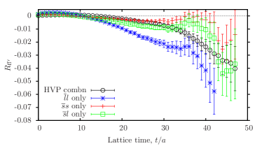
Figure 2: Ratios of disconnected correlators, $D^{\mathrm{ff^{\prime}}}$, to the connected correlator $C^{ll}$, as a function of time in lattice units. Open black circles show the combination of disconnected correlators needed for the hadronic vacuum polarization contribution to $a_{\mu,\mathrm{HVP}}$, described by eq. (8).

The Hadron Spectrum Collaboration has generated an ensemble of anisotropic gauge field configurations Lin et al. (2009) with the lattice spacing in the temporal direction about 3.5 times smaller than in the spatial directions. The gauge action is tree-level Symanzik-improved. The effects of $u,d$ and $s$ quark vacuum fluctuations are included, using a stout-smeared clover quark action. The $u$ and $d$ quarks are taken to be degenerate and have a mass approximately one-third that of the $s$ quark ($m_{\pi}$ = 391 MeV). The $s$ quark mass is tuned to be close to its physical value using the combination of meson masses $2m_{K}^{2}-m_{\pi}^{2}$ fixing the lattice spacing from the mass of the $\Omega$ baryon. In this study we use the $24^{3}\times 128$ lattices with mass parameters $a_{t}m_{l}=-0.0840$ and $a_{t}m_{s}=-0.0743$ and an inverse temporal lattice spacing of 5.6 GeV. The ensemble consists of 553 configurations.

The correlation functions employed in this study have a simple local spatial vector $\gamma_{i}$ operator at source and sink acting between quark and antiquark fields. The quark bilinear is constructed from distilled fields Peardon et al. (2009) $\tilde{\psi}=\Box\psi$ with

$$\Box_{xy}(t)=\sum_{k=1}^{N_{d}}\xi_{x}^{(k)}(t)\xi_{y}^{(k){\dagger}}(t).$$ (13)

Here $\xi_{k}(t)$ is the $k^{\rm th}$ lowest eigenvector of the gauge-covariant three-dimensional Laplace operator on time-slice $t$. In this study $N_{d}=162$. For the disconnected diagrams quark propagation from all time sources is computed.

The distillation method was developed primarily for hadron spectroscopy applications. Combined with the anisotropic lattices this enabled high-resolution and statistically precise determinations of disconnected diagrams Dudek et al. (2013a).

Using distilled quark fields is not ideal for our calculation because we wish to determine the time-moments of correlation functions constructed from local current operators that couple to the photon (as in eq. (4)). We will discuss this further below. A smeared correlation function, however, has the same exponential behaviour as a local correlation function at large times. It simply has a different normalisation for the amplitude. This can be fixed if we compare to correlation functions made from the same operator whose normalisation we know. Here we can compare the quark-line disconnected correlators to the connected correlators to fix the normalisation.

Figure 2 shows the ratio, $R_{\mathrm{f}\mathrm{f}^{\prime}}$, of each quark-line disconnected correlator $D^{\mathrm{ff^{\prime}}}$ to the connected correlator made of light quarks, $C^{ll}$, that uses the same operator at source and sink. The figure also includes the ratio for the combination of disconnected correlators needed for the HVP, as given in eq. (8). Correlators are calculated out to time slice $t=47$, which corresponds to 1.6 fm or $7/m_{\rho}$ for these parameters, giving ample time for ground-state properties to emerge and dominate the connected correlators. We see that all of the disconnected contributions become negative above a time-slice around 10. Not surprisingly $R_{ll}$ has the largest magnitude and $R_{ss}$ the smallest. $R_{ss}$ becomes consistent with zero above time-slice 30, where $R_{sl}$ also becomes small. Thus at large times the disconnected contribution to the HVP is dominated by the $ll$ component. At shorter times there is considerable cancellation between the off-diagonal $ls$ piece and the diagonal $ll$ and $ss$ pieces. Directly from this figure (and taking into account the factor of 1/5 from electric charge factors, see Section III) it is clear that we do not expect the disconnected contribution to $a_{\mu,\mathrm{HVP}}$ to amount to more than 1% of the connected $ll$ contribution.

In principle to determine the contribution of the disconnected correlators to $a_{\mu}$ we simply need to determine the time-moments using eq. (5). However Figure 2 shows that the correlators are too noisy at large times for this to be a feasible approach. Instead we must fit the correlators to their known physical behaviour – and this requires making combinations of connected and disconnected correlators which are physical – and use the fit results at large time values. This enables us to make use of the good statistical accuracy at short to medium times to fix the long time behaviour more precisely.

We first test this by studying the connected correlators, $C^{ll}$ and $C^{ss}$. The SU(2) isovector correlator, corresponding to flavour combinations $(\overline{u}\gamma_{i}u-\overline{d}\gamma_{i}d)/\sqrt{2}$, $\overline{u}\gamma_{i}d$ and $\overline{d}\gamma_{i}u$ has no quark-line disconnected contribution in the SU(2) limit. The ground-state of the connected light vector correlator $C^{ll}$ is then the $\rho$ meson at large times. The ground-state of the $C^{ss}$ correlator will be a version of the $\phi$ meson in which no mixing with other flavourless vector states is allowed. We expect this to be very close to the physical $\phi$ meson because $D^{ss}$ is so small.

We can test the robustness of our correlation function analysis which uses just a single current insertion, by comparing to the spectrum analyses of both the Hadron Spectrum and the HPQCD Collaborations. A multi-exponential model

$$\mathcal{C}_{\mathrm{fit}}(t)=\sum_{i=0}^{\mathrm{n_{exp}}}b_{i}^{2}e^{-E_{i}t},$$ (14)

where $b_{i}$ and $E_{i}$ are the amplitudes and masses respectively. We use a Bayesian approach Lepage et al. (2002) to constrain the parameters taking a prior of $0.85\pm 0.6\,\mathrm{GeV}$ on energy differences between the excitations and a width of 0.3 GeV on the ground-state mass. The amplitudes are given a prior of $0.1\pm 20$ where the normalisation of the correlators is such that the amplitudes of low-lying states are around 7–9. Our fit includes the full range of $t$ except for the first 3 values and stabilises after $\mathrm{n_{exp}}=3$ giving a ground-state mass in lattice units of $am_{\rho}=0.1512(4)$ and $am_{\phi}=0.1777(2)$. This is in good agreement with the Hadron Spectrum analysis in Ref. Dudek et al. (2013a) which used a large number of fermion bilinear operators in a variational basis. The same ensembles were used in a study of P-wave $I=1$ $\pi\pi$ scattering which gives a resonance mass of $a_{t}m_{R}=0.15085(18)(3)$ Dudek et al. (2013b). In addition, the value of $m_{\rho}$ at this value of $m_{\pi}$ is close to that expected from the HPQCD analysis of results at lighter values of $m_{\pi}$ Chakraborty et al. (2015).

Using the fits above we can readily determine the $\hat{\Pi}_{j}$ coefficients of eq. (7). To define a correlation function for any $t$ we combine the calculated correlator at short time separations with the model behaviour of eq. (14). We use

$$C(t)=\left\{\begin{array}[]{cc}C_{\mathrm{data}}(t),&t\leq t^{\ast}\\ \mathcal{C}_{\mathrm{fit}}(t),&t>t^{\ast}\end{array}\right..$$ (15)

From the calculation of the $\hat{\Pi}_{j}$ we obtain the contribution to $a_{\mu,\mathrm{HVP}}$ using eq. (1), with $Q^{2}_{s}=1/9$ and $Q^{2}_{l}=5/9$. We have tested that the results are insensitive to a number of variations of the method. These include: varying $t^{\ast}$ between 20 and 40; varying the total time length of the correlator used in the calculation of the moments from 95 upwards; varying the number of exponentials used in the fit result and varying the order of the Padé approximant between [1,1] and [2,2]. We find the ratio of the $\overline{s}s$ connected contribution to $a_{\mu,\mathrm{HVP}}$ to that of the $\overline{l}l$ connected contribution to be 0.125. This is in reasonable agreement with a linear extrapolation of the HPQCD results to the value of $m_{\pi}$ being used here, giving a value of around 0.15.

The isoscalar correlator, corresponding to flavour combination $(\overline{u}\gamma_{i}u+\overline{d}\gamma_{i}d)/\sqrt{2}$, has the same connected correlator contribution as for the $\rho$ but an additional quark-line disconnected contribution of $2{D}^{ll}$. The ground-state of this correlator is, to a good approximation, the $\omega$ meson. The $\omega$ meson is believed to contain a small admixture of $\overline{s}s$ with a mixing angle of a few degrees and this is seen in the Hadron Spectrum calculations Dudek et al. (2013a). This mixing occurs via the flavour off-diagonal disconnected correlators. We can include this effect, as well as establishing the large-time behaviour of all the correlators, by simultaneously fitting $ll$, $ss$ and $ls$ combinations of correlators with a single set of energy levels as in Dudek et al. (2013a). The $ll$ correlators consist of $C^{ll}+2D^{ll}$, the $ss$ correlators are $C^{ss}+D^{ss}$ and the $ls$ correlators are purely quark-line disconnected ($D^{ls}$). When $m_{u}$ and $m_{d}$ are not equal the $\omega$ can also mix with the neutral $\rho$ meson but, since we are working with $m_{u}=m_{d}$, we neglect this small effect.

We fit the 3 correlator combinations above simultaneously, using the fit form given in eq. (14) for the diagonal elements (but with different amplitudes for the $ll$ and $ss$ elements) and the form

$$\mathcal{C}^{sl}_{\rm fit}(t)=\sum_{i=0}^{\mathrm{n_{exp}}}d_{i}s_{i}e^{-E_{i}t}$$ (16)

for the off-diagonal element $D^{sl}$, where $d_{i}$ and $s_{i}$ do not need to be the same. All combinations share the parameters $E_{i}$. We take very similar priors to our earlier fits. However, we change the prior on the energy differences to of $700\pm 600\,\mathrm{MeV}$ to allow for the interleaving of excited $\phi$ and $\omega$ levels. We also fix a prior on the energy difference between the lowest energy (which we expect to correspond to the $\omega$) and the second lowest (which we expect to correspond to the mass of the $\phi$ meson). This difference is small here because the $\omega$ mass is relatively high at these values of $m_{l}$ (as we saw above for the $\rho$), and the $\phi$ mass is slightly lower than its physical value. We take a prior on the difference of the two energies of $170\pm 100\,\mathrm{MeV}$. The amplitude prior widths are again generally taken to be 20.0. However, we take a smaller prior width of 1.0 on $d_{i}$ and $s_{i}$ in eq. (16), reflecting the smaller size of the purely quark-line disconnected pieces. We also expect only a weak mixing between $\omega$ and $\phi$ states so that the amplitude of the $ss$ combination in the lowest mass state should be small and of the $ll$ combination in the second lowest mass state. We therefore fix the prior widths of these amplitudes also to be 1.0.

The fit, using a time range from 3 to 40 is stable from 6 exponentials upwards with a $\chi^{2}/\mathrm{dof}=1.1$ (Q=0.2). It gives $am_{\omega}=0.1537(10)$ and $am_{\phi}=0.1775(7)$. $am_{\omega}$ is somewhat lower than the value (0.1568(4)) obtained by the Hadron Spectum collaboration which included mixing between light and strange bilinears using more operators and the generalised eigenvalue fit method Dudek et al. (2013b). Our $m_{\omega}$ is higher than the corresponding $\rho$ mass by 14(6) MeV, compatible with the physical mass difference of 8 MeV Beringer et al. (2012). Note that isospin and electromagnetic effects are not included here. We obtain the same value of $am_{\phi}$ to that of simply fitting $C^{ss}$, so the quark-line disconnected contributions seem to have only a small impact, as expected.

From combinations of the fit results we can determine the large time behaviour of the disconnected correlators and therefore their time-moments. We again use the correlator data for $t\leq t^{\ast}$ as in eq. (15). For $D^{ll}$ we use correlator data up to $t^{\ast}$ and then half the difference of the ‘$\omega$’ and ‘$\rho$’ fits. For $D^{ss}$ we similarly take the correlator data up to $t^{\ast}$ and then take the difference of the full $\overline{s}s$ fit just described, and the result of simply fitting $C^{ss}$ above. In fact this gives a very similar result to that of simply including the time-moments of the $D^{ss}$ correlator. For $D^{sl}$ (=$D^{ls}$) we take the correlator data up to $t^{\ast}$ and then the fit result from eq. (16).

Combining this data using eq (8) with effective charge $Q=1/3$ gives a relative contribution to $a_{\mu}^{\mathrm{HVP}}$ of

$$\frac{a_{\mu,\mathrm{HVP}}^{\mathrm{disc}}}{a_{\mu,\mathrm{HVP}}^{ll,\mathrm{conn}}}=-0.14(5)\%.$$ (17)

We have checked that this result is robust (to 50%) to changing $t^{*}$; the order of the Padé approximant and the total time used in determining the time-moments.

The value is made up of -0.36(4)% from $D^{ll}$, +0.27(3)% from $D^{ls}$ (this has a coefficient of -2 in eq. (8)) and -0.05(1)% from $D^{ss}$.

V Discussion

Our result in eq. (17) shows that the disconnected piece of the HVP contribution to $a_{\mu}$ is very small. To obtain this result we have used vector current-current correlators using distilled quark fields and we have worked at rather large values of the $u/d$ quark mass at one value of the lattice spacing. We discuss each of these issues in turn, bearing in mind that the aim is to reduce the uncertainty of the disconnected contributions to the level of 1% of the connected contribution. If, as our result indicates, the size of the disconnected contribution is already itself of this order, then the relative accuracy in the value does not need to be very high.

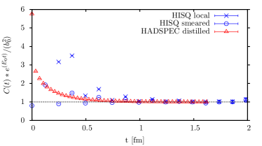
Figure 3: A comparison of local, smeared and distilled vector-vector connected correlators normalised to the contribution of the ground-state. Results for HISQ $u/d$ quarks compare a local operator at source and sink (blue crosses) with a smeared operator of Gaussian type and radius 3.75 at source and sink (blue open circles). Red open triangles give the Hadron Spectrum $C^{ll}$ results using distilled quark fields from 162 distillation vectors.

To understand the size of systematic error we could be making because of the use of distilled quark fields in the vector currents we can compare to results from the HPQCD collaboration. The HPQCD collaboration has connected $ll$ vector-vector correlators for both local and smeared operators using HISQ quarks on a range of gluon field ensembles at various values of $m_{l}$. The reason for using smeared operators in this case is to improve the fitted results for the ground-state behaviour in the local correlators Chakraborty et al. (2015). For a comparison between HPQCD and Hadron Spectrum results we want to choose an approximately matching spatial lattice spacing, since this controls the range of the smearing. The gluon field ensemble used here for the Hadron Spectrum results has a spatial lattice spacing of around 0.12 fm, based on an anisotropy of 3.444 Dudek et al. (2013b). This corresponds to the ‘coarse’ lattice spacing in the MILC gluon field ensembles used by the HPQCD collaboration Chakraborty et al. (2014). The MILC coarse ensemble with $m_{l}/m_{s}=0.2$ has a value for $m_{\pi}$ of 305 MeV Dowdall et al. (2013) which is somewhat lower than the Hadron Spectrum value used here of 391 MeV, but fairly similar. The smearing used by the HPQCD collaboration on these configurations uses a stride-2 covariant Laplacian, applying $[1+(r_{0}^{2}D^{2})/4n]^{n}$ to a local source. $r_{0}$ is set to 3.75 and $n$ to 30. The stride-2 Laplacian is needed to avoid mixing in other staggered tastes of vector meson Follana et al. (2007).

Figure 3 compares results for the HPQCD correlators using local and smeared operators on these coarse lattices. The quantity plotted is the correlator divided by the ground-state contribution so that at large times a result of 1 is guaranteed. The $x$-axis gives the time between source and sink in fm. We see that smeared correlators are closer to the large time behaviour at early times, although this is obscured somewhat by the oscillations present in vector correlators made with staggered quarks. Since the smearing is designed to increase the projection onto the ground-state it is not surprising that smeared correlators are saturated earlier by the ground-state. However there is little difference between smeared and local correlators beyond $t$ = 0.5 fm, equivalent to $2/m_{\rho}$ for this value of $m_{\pi}$. We can determine the contribution to $a_{\mu,\mathrm{HVP}}$ of the smeared and local correlators, using the method described in Section IV. If we normalise the two correlators by the ratio of their ground-state amplitudes, we find that the smeared correlators give a result for $a_{\mu,\mathrm{HVP}}$ that is about 10% low compared to the local result.

Figure 3 also compares the Hadron Spectrum results using distillation. Now the density of points in time is much higher, reflecting the finer discretisation of the time direction in the Hadron Spectrum lattices. The behaviour of the correlators is, however, fairly similar to that of the HPQCD smeared correlators (allowing for the oscillations in the staggered quark results). This gives some indication of the effective size of the Hadron Spectrum smearing. It also implies that we might expect the Hadron Spectrum results for contributions to $a_{\mu,\mathrm{HVP}}$ to be approximately 10% low compared to those obtained from local operators.

To understand to what extent the result might change as $m_{l}$ and hence $m_{\pi}$ is reduced to the physical value, we can compare the results from the Hadron Spectrum analysis Dudek et al. (2013a) at multiple values of $m_{\pi}$ to the picture found in experiment, bearing in mind that experiment also has effects from electromagnetism and $m_{u}\neq m_{d}$ that we are not including.

The impact of the disconnected correlator contributions to ground-state masses is to change the mass of the $\omega$ relative to the $\rho$ and to change the mixing between the $\phi$ and the $\omega$. The Hadron Spectrum analysis finds, even at $m_{\pi}>$ 391 MeV, a picture that is qualitatively and quantitatively very similar to experiment, except that $m_{\rho}$ is too heavy. The impact of the $\rho$ mass being too heavy is largely removed by the fact that we take a ratio of the disconnected contribution to that of the connected contribution. The $\omega$ is found to be slightly heavier than the $\rho$ and the mixing between the $\omega$ and $\phi$ is a few degrees. Excited state masses also agree well with experiment. The mass difference between $\omega$ and $\rho$ is seen to increase slightly as $m_{\pi}$ falls and the mixing angle with the $\phi$ also increases. Large changes are not to be expected, however, if the results are to be compatible with experiment in the continuum and chiral limits. The masses of the $\eta$ and $\eta^{\prime}$, whose correlators have large contributions from quark-line disconnected diagrams, also show good (at the 10% level) agreement with experiment. This demonstrates that quark-line disconnected contributions are not unduly distorted at heavy values of $m_{\pi}$.

The discussion above relates to meson masses which test the correlator time-dependence. We also have to worry about the correlator amplitudes which would be tested through the determination of decay constants. The most that we can do here is test ratios of decay constants because we do not have normalisation factors for our currents. Our fit results for the $\phi$ and $\rho$ yield a ratio for the decay constants of 1.03. This is compatible with experimental results for the relative leptonic widths, given the uncertainties for the $\rho$ discussed in Section III. Our fit results for the $\rho$ and $\omega$ give decay constants that are the same, up to 2% uncertainties. Again this is compatible with experiment.

The key effect that is $m_{\pi}$-dependent and that is being underestimated in these lattice QCD results is that of the $\pi\pi$ contribution, both resonant, from $\rho$ decay, and non-resonant. From Section III we estimated that the disconnected $\pi\pi$ contribution to $a_{\mu,\mathrm{HVP}}$ is -1%. This uncertainty is larger than any of the $m_{\pi}$-dependent effects discussed above.

The fact that only one value of the lattice spacing is being used means that we have no direct way of testing for discretisation effects. The discretisation of QCD used for the Hadron Spectrum results has discretisation errors in principle of order $\alpha_{s}(\Lambda a_{s})$ and $(\Lambda a_{s})^{2}$. Here $\Lambda$ is a suitable QCD scale that sets the size of discretisation effects, say 400 MeV. $a_{s}$ is the spatial lattice spacing, $a_{s}^{-1}$ = 1.6 GeV. We might therefore expect discretisation errors of 5–10%. This is consistent with the comparison to HPQCD results where three values of the lattice spacing have been used for connected correlator calculations so that a clear continuum limit can be taken (and in fact only very small discretisation errors are evident). The Hadron Spectrum results for $m_{\rho}$ and $m_{\phi}$ are consistent with those from HPQCD at a similar value for $m_{\pi}$ within possible 5–10% discretisation errors.

We conclude that uncertainties from the effect of distillation and the use of relatively heavy $\pi$ mesons at one value of the lattice spacing could amount to a total of 50% of the very small value for the ratio of disconnected to connected contributions to the HVP found in Section IV. A larger uncertainty comes from the $\pi\pi$ contributions that are badly distorted at heavy $m_{\pi}$ and this will dominate our final uncertainty.

VI Conclusions

The ultimate aim of lattice QCD calculations of $a_{\mu,\mathrm{HVP}}$ is to improve on results from using, for example, $\sigma(e^{+}e^{-}\rightarrow\mathrm{hadrons})$ that are able to achieve an uncertainty of below 1%. We are not at that stage yet. The ETM Collaboration are the first to include a full calculation from connected correlators including $u/d$, $s$ and $c$ quarks Burger et al. (2014) and quote a 4% uncertainty that includes lattice systematic uncertainties. A 1% uncertainty has now been achieved on the $s$ quark connected contribution Chakraborty et al. (2014) and an improved accuracy on the total $u/d$, $s$ and $c$ quark connected correlator calculation is within reach Chakraborty et al. (2015). However neither of these calculations includes the impact of quark-line disconnected correlators. Although the total disconnected contribution to $a_{\mu,\mathrm{HVP}}$ is expected to be small, it must either be evaluated or constrained at the level of 1% of the total if it is not to undermine our ability to reach the desired accuracy on $a_{\mu,\mathrm{HVP}}$ from lattice QCD calculations.

Here we have given the first estimates of the quark-line disconnected contribution to $a_{\mu,\mathrm{HVP}}$ based on disconnected correlators with a clear signal. We determine the disconnected contribution as a ratio to the connected $u/d$ contribution so that a number of systematic errors cancel or are reduced. The results show that the disconnected contribution is indeed small, at -0.15% of the connected contribution at the relatively heavy value of $m_{\pi}$ (391 MeV) used here. We estimate the uncertainty in this contribution as 1% of the connected contribution coming largely from $\pi\pi$ effects that are badly distorted at heavy $m_{\pi}$. The value is consistent with a simple phenomenological bound based on the experimental properties of the $\rho$ and $\omega$ mesons which gives, again as a ratio to the connected contribution, between 0 and -2%.

In future a more accurate calculation of the quark-line disconnected contributions will be possible with smaller values of $m_{\pi}$, going down to the physical point, and on finer lattices. This should enable us eventually to pin down these contributions at the 0.1% level. The result given here however is enough to make clear that the quark-line disconnected contribution to $a_{\mu,\mathrm{HVP}}$ can safely be assessed to be at the level of 1% of the connected contribution. It will not therefore prevent us, for now, in reaching an accuracy on the total $a_{\mu,\mathrm{HVP}}$ of around 1% from lattice QCD.

Acknowledgements. We are grateful to the Hadron Spectrum Collaboration for the correlators used here and to C. Bernard for useful discussions. Chroma Edwards and Joo (2005) and QUDA Clark et al. (2010); Babich et al. (2010) were used on clusters at Jefferson Laboratory under the USQCD Initiative and the LQCD ARRA project. Gauge configurations were generated using resources awarded from the U.S. Department of Energy INCITE program at Oak Ridge National Lab, the NSF Teragrid at the Texas Advanced Computer Center and the Pittsburgh Supercomputer Center as well as at Jefferson Lab. Calculations were also done on the Darwin Supercomputer as part of STFC’s DiRAC facility jointly funded by STFC, BIS and the Universities of Cambridge and Glasgow. This work was funded by the Gilmour bequest to the University of Glasgow, Science Foundation Ireland (grant 11-RFP.1-PHY-3201), the Science and Technology Facilities Council, the Royal Society, the Wolfson Foundation and the National Science Foundation.

References

- Bennett et al. (2006) G. Bennett et al. (Muon G-2 Collaboration), Phys.Rev. D73, 072003 (2006), eprint hep-ex/0602035.
- Aoyama et al. (2012) T. Aoyama, M. Hayakawa, T. Kinoshita, and M. Nio, Phys.Rev.Lett. 109, 111808 (2012), eprint 1205.5370.
- Hagiwara et al. (2011) K. Hagiwara, R. Liao, A. D. Martin, D. Nomura, and T. Teubner, J.Phys. G38, 085003 (2011), eprint 1105.3149.
- Davier et al. (2011) M. Davier, A. Hoecker, B. Malaescu, and Z. Zhang, Eur.Phys.J. C71, 1515 (2011), eprint 1010.4180.
- Blum et al. (2013) T. Blum, A. Denig, I. Logashenko, E. de Rafael, B. Lee Roberts, et al. (2013), eprint 1311.2198.
- Benayoun et al. (2015) M. Benayoun, P. David, L. DelBuono, and F. Jegerlehner (2015), eprint 1507.02943.
- Blum (2003) T. Blum, Phys.Rev.Lett. 91, 052001 (2003), eprint hep-lat/0212018.
- Burger et al. (2014) F. Burger, X. Feng, G. Hotzel, K. Jansen, M. Petschlies, and D. B. Renner (ETM), JHEP 02, 099 (2014), eprint 1308.4327.
- Chakraborty et al. (2014) B. Chakraborty, C. T. H. Davies, G. C. Donald, R. J. Dowdall, J. Koponen, G. P. Lepage, and T. Teubner (HPQCD), Phys. Rev. D89, 114501 (2014), eprint 1403.1778.
- Guelpers et al. (2014) V. Guelpers, A. Francis, B. Jaeger, H. Meyer, G. von Hippel, and H. Wittig, PoS LATTICE2014, 128 (2014), eprint 1411.7592.
- Peardon et al. (2009) M. Peardon, J. Bulava, J. Foley, C. Morningstar, J. Dudek, R. G. Edwards, B. Joo, H.-W. Lin, D. G. Richards, and K. J. Juge (Hadron Spectrum), Phys. Rev. D80, 054506 (2009), eprint 0905.2160.
- Dudek et al. (2013a) J. J. Dudek, R. G. Edwards, P. Guo, and C. E. Thomas (Hadron Spectrum), Phys. Rev. D88, 094505 (2013a), eprint 1309.2608.
- Lautrup et al. (1972) B. e. Lautrup, A. Peterman, and E. de Rafael, Phys. Rept. 3, 193 (1972).
- Allison et al. (2008) I. Allison et al. (HPQCD Collaboration), Phys.Rev. D78, 054513 (2008), eprint 0805.2999.
- McNeile et al. (2010) C. McNeile, C. Davies, E. Follana, K. Hornbostel, and G. Lepage (HPQCD Collaboration), Phys.Rev. D82, 034512 (2010), eprint 1004.4285.
- (16) The Padé approximant of a function is a ratio of polynomials in , of order in the numerator and in the denominator, whose Taylor expansion is the same as that of through order .
- Follana et al. (2007) E. Follana, Q. Mason, C. Davies, K. Hornbostel, G. P. Lepage, et al. (HPQCD and UKQCD Collaborations), Phys.Rev. D75, 054502 (2007), eprint hep-lat/0610092.
- Kuhn et al. (2007) J. H. Kuhn, M. Steinhauser, and C. Sturm, Nucl. Phys. B778, 192 (2007), eprint hep-ph/0702103.
- Beringer et al. (2012) J. Beringer et al. (Particle Data Group), Phys.Rev. D86, 010001 (2012).
- Jegerlehner and Szafron (2011) F. Jegerlehner and R. Szafron, Eur. Phys. J. C71, 1632 (2011), eprint 1101.2872.
- Della Morte and Juttner (2010) M. Della Morte and A. Juttner, JHEP 11, 154 (2010), eprint 1009.3783.
- Lin et al. (2009) H.-W. Lin et al. (Hadron Spectrum), Phys. Rev. D79, 034502 (2009), eprint 0810.3588.
- Lepage et al. (2002) G. P. Lepage, B. Clark, C. T. H. Davies, K. Hornbostel, P. B. Mackenzie, C. Morningstar, and H. Trottier, Nucl. Phys. Proc. Suppl. 106, 12 (2002), eprint hep-lat/0110175.
- Dudek et al. (2013b) J. J. Dudek, R. G. Edwards, and C. E. Thomas (Hadron Spectrum), Phys. Rev. D87, 034505 (2013b), [Erratum: Phys. Rev.D90,no.9,099902(2014)], eprint 1212.0830.
- Chakraborty et al. (2015) B. Chakraborty, C. Davies, P. G. de Oliveira, J. Koponen, and G. P. Lepage, PoS LATTICE2015, 108 (2015), eprint 1511.05870.
- Dowdall et al. (2013) R. Dowdall, C. Davies, G. Lepage, and C. McNeile (HPQCD Collaboration), Phys.Rev. D88, 074504 (2013), eprint 1303.1670.
- Edwards and Joo (2005) R. G. Edwards and B. Joo (SciDAC, LHPC, UKQCD), Nucl. Phys. Proc. Suppl. 140, 832 (2005), eprint hep-lat/0409003.
- Clark et al. (2010) M. A. Clark, R. Babich, K. Barros, R. C. Brower, and C. Rebbi, Comput. Phys. Commun. 181, 1517 (2010), eprint 0911.3191.
- Babich et al. (2010) R. Babich, M. A. Clark, and B. Joo, in SC 10 (Supercomputing 2010) New Orleans, Louisiana, November 13-19, 2010 (2010), eprint 1011.0024.