The Riemann Solver for Traffic Flow at an Intersection with Buffer of Vanishing Size

Abstract

The paper examines the model of traffic flow at an intersection introduced in [2], containing a buffer with limited size. As the size of the buffer approach zero, it is proved that the solution of the Riemann problem with buffer converges to a self-similar solution described by a specific Limit Riemann Solver (LRS). Remarkably, this new Riemann Solver depends Lipschitz continuously on all parameters.

1 Introduction

Starting with the seminal papers by Lighthill, Witham, and Richards [12, 13], traffic flow on a single road has been modeled in terms of a scalar conservation law:

$$\rho_{t}+(v(\rho)\rho)_{x}~{}=~{}0\,.$$ (1.1)

Here $\rho$ is the density of cars, while $v(\rho)$ is their velocity, which we assume depends of the density alone. To describe traffic flow on an entire network of roads, one needs to further introduce a set of boundary conditions at road junctions [7]. These conditions should relate the traffic densities on incoming roads $i\in{\cal I}$ and outgoing roads $j\in{\cal O}$, depending on two main parameters:

• Driver’s turning preferences. For every $i,j$, one should specify the fraction $\theta_{ij}\in[0,1]$ of drivers arriving to from the $i$-th road, who wish to turn into the $j$-th road.

• Relative priorities assigned to different incoming roads. If the intersection is congested, these describe the maximum influx of cars arriving from each road $i\in{\cal I}$, allowed to cross the intersection.

Various junction models of have been proposed in the literature [4, 5, 7, 9]. See also [1] for a survey. A convenient approach is to introduce a Riemann Solver, i.e. a rule that specifies how to construct the solution in the special case where the initial data is constant on every incoming and each outgoing road. As shown in [4], as soon as a Riemann Solver is given, the general Cauchy problem for traffic flow near a junction can be uniquely solved (under suitable assumptions).

The recent counterexamples in [3] show that, on a network of roads, in general the Cauchy problem can be ill posed. Indeed, two distinct solutions can be constructed for the same measurable initial data. On a network with several nodes, nonuniqueness can occur even if the initial data have small total variation. To readdress this situation, in [2] an alternative intersection model was proposed, introducing a buffer of limited capacity at each road junction. For this new model, given any ${\bf L}^{\infty}$ initial data, the Cauchy problem has a unique solution, which is robust w.r.t. perturbations of the data. Indeed, one has continuous dependence even w.r.t. the topology of weak convergence.

A natural question, addressed in the present paper, is what happens in the limit as the size of the buffer approaches zero. For Riemann initial data, constant along each incoming and outgoing road, we show that this limit is described by a Limit Riemann Solver (LRS) which can be explicitly determined. See (2.15)–(2.17) in Section 2.

We recall that, in a model without buffer, the initial conditions consist of the constant densities $\rho^{\diamondsuit}_{k}$ on all incoming and outgoing roads $k\in{\cal I}\cup{\cal O}$, together with the drivers’ turning preferences $\theta_{ij}^{\diamondsuit}$. On the other hand, in the model with buffer, these initial conditions comprise also the length of the queues $q_{j}^{\diamondsuit}$, $j\in{\cal O}$, inside the buffer. One can think of $q^{\diamondsuit}_{j}$ as the number of cars already inside the intersection (say, a traffic circle) at time $t=0$, waiting to access the outgoing road $j$. Our main results can be summarized as follows.

• For any given Riemann data $\rho^{\diamondsuit}_{k},\,\theta_{ij}^{\diamondsuit}$, one can choose initial queue sizes $q_{j}^{\diamondsuit}$ such that, for all $t>0$ the solution of the problem with buffer is exactly the same as the solution determined by the Riemann Solver (LRS).

• For any Riemann data $\rho^{\diamondsuit}_{k},\,\theta_{ij}^{\diamondsuit}$, and any initial queue sizes $q_{j}^{\diamondsuit}$, as $t\to\infty$ the solution of the problem with buffer approaches asymptotically the solution determined by the Riemann Solver (LRS).

Using the fact that the conservation laws (1.1) are invariant under space and time rescalings, from (ii) we obtain a convergence result as the size of the buffer approaches zero.

Our present results apply only to solutions of the Riemann problem, i.e. with traffic density which is initially constant along each road. Indeed, for a general Cauchy problem the counterexamples in [3] remain valid also for the Riemann Solver (LRS), showing that the initial-value problem with measurable initial data can be ill posed. Hence no convergence result can be expected. This should not appear as a paradox: for every positive size of the buffer, the Cauchy problem has a unique solution, depending continuously on the initial data. However, as the size of the buffer approaches zero, the solution can become more and more sensitive to small changes in the initial conditions. In the limit, uniqueness is lost.

An extension of our results may be possible in the case of initial data with bounded variation, for a network containing one single node. In view of the results in [4, 7], we conjecture that in this case the solution to the Cauchy problem with buffer converges to the solution determined by the Riemann Solver (LRS).

2 Statement of the main results

Consider a family of $n+m$ roads, joining at a node. Indices $i\in\{1,\ldots,m\}={\cal I}$ denote incoming roads, while indices $j\in\{m+1,\ldots,m+n\}={\cal O}$ denote outgoing roads. On the $k$-th road, the density of cars $\rho_{k}(t,x)$ is governed by the scalar conservation law

$$\rho_{t}+f_{k}(\rho)_{x}~{}=~{}0\,.$$ (2.1)

Here $t\geq 0$, while $x\in\,]-\infty,0]$ for incoming roads and $x\in[0,\,+\infty[\,$ for outgoing roads. The flux function is $f_{k}(\rho)=\rho\,v_{k}(\rho)$, where $v_{k}(\rho)$ is the speed of cars on the $k$-th road. We assume that each flux function $f_{k}$ satisfies

$$f_{k}\in{\cal C}^{2},\qquad f_{k}(0)~{}=~{}f_{k}(\rho_{k}^{jam})~{}=~{}0,\qquad f_{k}^{\prime\prime}(\rho)~{}<~{}0\qquad\hbox{for all}~{}~{}\rho\in[0,\rho_{k}^{jam}],$$ (2.2)

where $\rho_{k}^{jam}$ is the maximum possible density of cars on the $k$-th road. Intuitively, this can be thought as a bumper-to-bumper packing, so that the speed of cars is zero. For a given road $k\in\{1,\ldots,m+n\}$, we denote by

$$f_{k}^{max}~{}\doteq~{}\max_{s}~{}f_{k}(s)$$

the maximum flux and

$$\rho_{k}^{max}~{}\doteq~{}\hbox{arg}\!\max_{s}~{}f_{k}(s)$$ (2.3)

the traffic density corresponding to this maximum flux (see Fig. 1).

Figure 1: The flux $f_{k}$ as a function of the density $\rho$, along the $k$-th road.

Moreover, we say that

$$\begin{array}[]{rl}\rho~{}~{}\hbox{is a {\bf free} state if}&~{}~{}\rho\in\,[0,\,\rho_{k}^{max}]\,,\cr\rho~{}~{}\hbox{is a {\bf congested} state if}&~{}~{}\rho\in~{}[\rho_{k}^{max},\,\rho_{k}^{jam}]\,.\end{array}$$

Given initial data on each road

$$\rho_{k}(0,x)~{}=~{}\rho_{k}^{\diamondsuit}(x)\qquad\qquad k=1,\ldots,m+n,$$ (2.4)

in order to determine a unique solution to the Cauchy problem we must supplement the conservation laws (2.1) with a suitable set of boundary conditions. These provide additional constraints on the limiting values of the vehicle densities

$$\bar{\rho}_{k}(t)~{}\doteq~{}\lim_{x\to 0}\rho_{k}(t,x)\qquad\qquad k=1,\ldots,m+n$$ (2.5)

near the intersection. In a realistic model, these boundary conditions should depend on:

• Relative priority given to incoming roads. For example, if the intersection is regulated by a crosslight, the flow will depend on the fraction $\eta_{i}\in\,]0,1[\,$ of time when cars arriving from the $i$-th road get a green light.

• Drivers’ choices. For every $i\in{\cal I}$, $j\in{\cal O}$, these are modeled by assigning the fraction $\theta_{ij}\in[0,1]$ of drivers arriving from the $i$-th road who choose to turn into the $j$-th road. Obvious modeling considerations imply

  $$\theta_{ij}\in[0,1]\,,\qquad\qquad\sum_{j\in{\cal O}}\theta_{ij}~{}=~{}1\quad\hbox{for each}~{}i\in{\cal I}\,.$$ (2.6)

  Since we are only interested in the Riemann problem, throughout the following we shall assume that the $\theta_{ij}$ are given constants, satisfying (2.6).

In [2] a model of traffic flow at an intersection was introduced, including a buffer of limited capacity. The incoming fluxes of cars toward the intersection are constrained by the current degree of occupancy of the buffer. More precisely, consider an intersection with $m$ incoming and $n$ outgoing roads. The state of the buffer at the intersection is described by an $n$-vector

$${\bf q}~{}=~{}(q_{j})_{j\in{\cal O}}\,.$$

Here $q_{j}(t)$ is the number of cars at the intersection waiting to enter road $j\in{\cal O}$ (in other words, the length of the queue in front of road $j$). Boundary values at the junction will be denoted by

$$\left\{\begin{array}[]{rl}\bar{\theta}_{ij}(t)&\doteq~{}\lim_{x\to 0-}\theta_{ij}(t,x),\qquad i\in{\cal I},~{}j\in{\cal O}\,,\cr\cr\bar{\rho}_{i}(t)&\doteq~{}\lim_{x\to 0-}\rho_{i}(t,x),\qquad i\in{\cal I}\,,\cr\cr\bar{\rho}_{j}(t)&\doteq~{}\lim_{x\to 0+}\rho_{j}(t,x),\qquad j\in{\cal O}\,,\cr\cr\bar{f}_{i}(t)&\doteq~{}f_{i}(\bar{\rho}_{i}(t))~{}=~{}\lim_{x\to 0-}f_{i}(\rho_{i}(t,x)),\qquad i\in{\cal I}\,,\cr\cr\bar{f}_{j}(t)&\doteq~{}f_{j}(\bar{\rho}_{j}(t))~{}=~{}\lim_{x\to 0+}f_{j}(\rho_{j}(t,x)),\qquad j\in{\cal O}\,.\end{array}\right.$$ (2.7)

Conservation of the total number of cars implies

$$\dot{q}_{j}(t)~{}=~{}\sum_{i\in{\cal I}}\bar{f}_{i}(t)\bar{\theta}_{ij}-\bar{f}_{j}(t)\qquad\qquad\hbox{for all}~{}j\in{\cal O}\,,$$ (2.8)

at a.e. time $t\geq 0$. Here and in the sequel, the upper dot denotes a derivative w.r.t. time. Following [7], we define the maximum possible flux at the end of an incoming road as

$$\omega_{i}~{}=~{}\omega_{i}(\bar{\rho}_{i})~{}\doteq~{}\left\{\begin{array}[]{rl}f_{i}(\bar{\rho}_{i})&\hbox{if~{}$\bar{\rho}_{i}$ is a free state},\cr\cr f_{i}^{max}&\hbox{if~{}$\bar{\rho}_{i}$ is a congested state},\end{array}\right.\qquad\quad i\in{\cal I}\,.$$ (2.9)

This is the largest flux $f_{i}(\rho)$ among all states $\rho$ that can be connected to $\bar{\rho}_{i}$ with a wave of negative speed. Notice that the two right hand sides in (2.9) coincide if $\bar{\rho}_{i}=\rho_{i}^{max}$.

Similarly, we define the maximum possible flux at the beginning of an outgoing road as

$$\omega_{j}~{}=~{}\omega_{j}(\bar{\rho}_{j})~{}\doteq~{}\left\{\begin{array}[]{rl}f_{j}(\bar{\rho}_{j})&\hbox{if~{}$\bar{\rho}_{j}$ is a congested state},\cr\cr f_{j}^{max}&\hbox{if~{}$\bar{\rho}_{j}$ is a free state},\end{array}\right.\qquad\quad j\in{\cal O}\,.$$ (2.10)

As in [2], we assume that the junction contains a buffer of size $M$. Incoming cars are admitted at a rate depending of the amount of free space left in the buffer, regardless of their destination. Once they are within the intersection, cars flow out at the maximum rate allowed by the outgoing road of their choice. Single Buffer Junction (SBJ).   Consider a constant $M>0$, describing the maximum number of cars that can occupy the intersection at any given time, and constants $c_{i}>0$, $i\in{\cal I}$, accounting for priorities given to different incoming roads.

We then require that the incoming fluxes $\bar{f}_{i}$ satisfy

$$\bar{f}_{i}~{}=~{}\min~{}\left\{\omega_{i}\,,~{}~{}c_{i}\Big{(}M-\sum_{j\in{\cal O}}q_{j}\Big{)}\right\},\qquad\qquad i\in{\cal I}\,.$$ (2.11)

In addition, the outgoing fluxes $\bar{f}_{j}$ should satisfy

$$\left\{\begin{array}[]{l}\hbox{if $q_{j}>0$, then $\bar{f}_{j}=\omega_{j}$,}\cr\cr\hbox{if $q_{j}=0$, then $\bar{f}_{j}=\min\Big{\{}\omega_{j},~{}\sum_{i\in{\cal I}}\bar{f}_{i}\bar{\theta}_{ij}\Big{\}}$,}\end{array}\right.\qquad\qquad j\in{\cal O}\,.$$ (2.12)

Here $\omega_{i}=\omega_{i}(\bar{\rho}_{i})$ and $\omega_{j}=\omega_{j}(\bar{\rho}_{j})$ are the maximum fluxes defined at (2.9)-(2.10). Notice that (SBJ) prescribes all the boundary fluxes $\bar{f}_{k}$, $k\in{\cal I}\cup{\cal O}$, depending on the boundary densities $\bar{\rho}_{k}$. It is natural to assume that the constants $c_{i}$ satisfy the inequalities

$$c_{i}M~{}>~{}f_{i}^{max}\qquad\quad\hbox{for all}~{}i\in{\cal I}\,.$$ (2.13)

These conditions imply that, when the buffer is empty, cars from all incoming roads can access the intersection with the maximum possible flux (2.9). The analysis in [2] shows that, with the above boundary conditions, the Cauchy problem on a network of roads has a unique solution, continuously depending on the initial data.

The main goal of this paper is to understand what happens when the size of the buffer approaches zero. More precisely, assume that (2.11) is replaced by

$$\bar{f}_{i}~{}=~{}\min~{}\left\{\omega_{i}\,,~{}~{}{c_{i}\over\varepsilon}\Big{(}M\varepsilon-\sum_{j\in{\cal O}}q_{j}\Big{)}\right\},\qquad\qquad i\in{\cal I}\,.$$ (2.14)

Notice that (2.14) models a buffer with size $M\varepsilon$. When $\sum_{j}q_{j}=M\varepsilon$, the buffer is full and no more cars are admitted to the intersection.

We will show that, as $\varepsilon\to 0$, the limit of solutions to the Riemann problem with buffer of vanishing size can be described by a specific Limit Riemann Solver.

• At time $t=0$, let the constant densities $\rho_{i}^{\diamondsuit}$, $\rho_{j}^{\diamondsuit}$ be given, together with drivers’ preferences $\theta_{ij}$,   $i\in{\cal I}$, $j\in{\cal O}$.

  Let $\omega_{i}^{\diamondsuit}=\omega_{i}(\rho_{i}^{\diamondsuit})$ and $\omega_{j}^{\diamondsuit}=\omega_{j}(\rho_{j}^{\diamondsuit})$ be the corresponding maximum possible fluxes at the boundary of the incoming and outgoing roads, as in (2.9)-(2.10). Consider the one-parameter curve

  $$s~{}\mapsto~{}\gamma(s)~{}=~{}(\gamma_{1}(s),\ldots,\gamma_{m}(s)),$$

  where

  $$\gamma_{i}(s)~{}\doteq~{}\min\{c_{i}s\,,~{}\omega_{i}^{\diamondsuit}\}.$$

  Then for $t>0$ the Riemann problem is solved by the incoming fluxes

  $$\bar{f}_{i}~{}=~{}\gamma_{i}(\bar{s}),$$ (2.15)

  where

  $$\bar{s}~{}=~{}\max~{}\left\{s\in[0,M]\,;~{}~{}\sum_{i\in{\cal I}}\gamma_{i}(s)\,\theta_{ij}~{}\leq~{}\omega_{j}^{\diamondsuit}\quad\hbox{for all}~{}j\in{\cal O}\right\}.$$ (2.16)

  In turn, by the conservation of the number of drivers, the outgoing fluxes are

  $$\bar{f}_{j}~{}=~{}\sum_{i\in{\cal I}}\bar{f}_{i}\,\theta_{ij}\qquad\qquad j\in{\cal O}\,.$$ (2.17)

By specifying all the incoming and outgoing fluxes $\bar{f}_{i},\bar{f}_{j}$ at the intersection, the entire solution of the Riemann problem is uniquely determined. Indeed:

• For an incoming road $i\in{\cal I}$, there exists a unique boundary state $\rho_{i}^{0}=\rho_{i}(t,0-)$ such that $f_{i}(\rho_{i}^{0})=\bar{f}_{i}$ and moreover

  • If $\bar{f}_{i}=f_{i}(\rho_{i}^{\diamondsuit})$, then $\rho_{i}^{0}=\rho_{i}^{\diamondsuit}$. In this case the density of cars on the $i$-th road remains constant: $\rho_{i}(t,x)\equiv\rho_{i}^{\diamondsuit}$.

  • If $\bar{f}_{i}\not=f_{i}(\rho_{i}^{\diamondsuit})$, then the solution to the Riemann problem

    $$\rho_{t}+f_{i}(\rho)_{x}~{}=~{}0,\qquad\qquad\rho(0,x)~{}=~{}\left\{\begin{array}[]{rl}\rho_{i}^{\diamondsuit}&\qquad\hbox{if}~{}~{}x<0,\\[8.53581pt] \rho_{i}^{0}&\qquad\hbox{if}~{}~{}x>0,\end{array}\right.$$ (2.18)

    contains only waves with negative speed. In this case, the density of cars on the $i$-th road coincides with the solution of (2.18), for $x<0$.

• For an outgoing road $j\in{\cal O}$, there exists a unique boundary state $\rho_{j}^{0}=\rho_{j}(t,0-)$ such that $f_{j}(\rho_{j}^{0})=\bar{f}_{j}$ and moreover

  • If $\bar{f}_{j}=f_{j}(\rho_{j}^{\diamondsuit})$, then $\rho_{j}^{0}=\rho_{j}^{\diamondsuit}$. In this case the density of cars on the $j$-th road remains constant: $\rho_{j}(t,x)\equiv\rho_{j}^{\diamondsuit}$.

  • If $\bar{f}_{j}\not=f_{j}(\rho_{j}^{\diamondsuit})$, then the solution to the Riemann problem

    $$\rho_{t}+f_{j}(\rho)_{x}~{}=~{}0,\qquad\qquad\rho(0,x)~{}=~{}\left\{\begin{array}[]{rl}\rho_{j}^{0}&\qquad\hbox{if}~{}~{}x<0,\\[8.53581pt] \rho_{j}^{\diamondsuit}&\qquad\hbox{if}~{}~{}x>0,\end{array}\right.$$ (2.19)

    contains only waves with positive speed. In this case, the density of cars on the $i$-th road coincides with the solution of (2.19), for $x>0$.

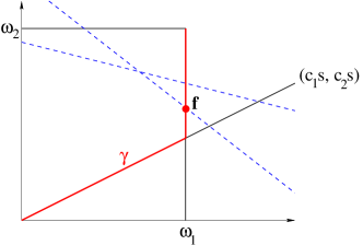
Figure 2: Constructing the solution of the the Riemann problem, according to the limit Riemann solver (LRS), with two incoming and two outgoing roads. The vector ${\bf f}=(\bar{f}_{1},\bar{f}_{2})$ of incoming fluxes is the largest point on the curve $\gamma$ that satisfies the two constraints $\sum_{i\in{\cal I}}\gamma_{i}(s)\theta_{ij}\leq\omega_{j}$, $j\in{\cal O}$.

Remark 1. For the Riemann Solver constructed in [3], the fluxes $\bar{f}_{k}$ are locally Hölder continuous functions of the data $\rho_{k}^{\diamondsuit},\theta_{ij}$, on the domain where $\theta_{ij}>0$, $\omega_{j}>0$ for all $j\in{\cal O}$.
The Riemann Solver (LRS) has even better regularity properties. Namely, the fluxes $\bar{f}_{k}$ defined at (2.15)–(2.17) are locally Lipschitz continuous functions of $\rho_{k}^{\diamondsuit},\theta_{ij}$. Unfortunately, as remarked earlier, this additional regularity is still not sufficient to guarantee the well-posedness of the Cauchy problem, for general measurable initial data. Our first result refers to “well prepared” initial data, where the initial lengths of the queues are suitably chosen. Theorem 1. Let the assumptions (2.2), (2.13) hold. Let Riemann data

$$\rho_{k}(0,x)=\rho_{k}^{\diamondsuit}\in[0,\rho_{k}^{jam}[\,,\qquad\qquad k\in{\cal I}\cup{\cal O},$$ (2.20)

be assigned along each road, together with drivers’ turning preferences $\theta_{ij}$.

Then one can choose initial values $q_{j}^{\diamondsuit}$, $j\in{\cal O}$ for the queues inside the buffer in such a way that the solution to the Riemann problem with buffer coincides with the self-similar solution determined by the Limit Riemann Solver (LRS). Our second result covers the general case, where the initial sizes of the queues are given arbitrarily, and the solution of the initial value problem with buffer is not self-similar. Theorem 2. Let the assumptions (2.2), (2.13) hold. Let Riemann data (2.20) be assigned along each road, together with drivers’ turning preferences $\theta_{ij}>0$ and initial queue sizes

$$q_{j}(0)~{}=~{}q_{j}^{\diamondsuit}\,,\qquad\hbox{with}\quad\sum_{j\in{\cal O}}q_{j}^{\diamondsuit}~{}<~{}M.$$ (2.21)

Then, as $t\to+\infty$, the solution $(\rho_{k}(t,x))_{k\in{\cal I}\cup{\cal O}}$ to the Riemann problem with buffer asymptotically converges to the self-similar solution $(\hat{\rho}_{k}(t,x))_{k\in{\cal I}\cup{\cal O}}$ determined by the Limit Riemann Solver (LRS). More precisely:

$$\lim_{t\to+\infty}~{}{1\over t}\left(\sum_{i\in{\cal I}}\int_{-\infty}^{0}|\rho_{i}(t,x)-\hat{\rho}_{i}(t,x)|\,dx+\sum_{j\in{\cal O}}\int_{0}^{+\infty}|\rho_{j}(t,x)-\hat{\rho}_{j}(t,x)|\,dx\right)~{}=~{}0.$$ (2.22)

A proof of the above theorems will be given in Sections 4 and 5, respectively. By an asymptotic rescaling of time and space, using Theorem 2 we can describe the behavior of the solution to a Riemann problem, as the size of the buffer approaches zero. Corollary (limit behavior for a buffer of vanishing size). Let $f_{k},\theta_{ij},c_{i},M$ be as in Theorem 2. Let Riemann data (2.20) be assigned along each road, together with drivers’ turning preferences $\theta_{ij}>0$ and initial queue sizes as in (2.21).

For $\varepsilon>0$, let $(\rho^{\varepsilon}_{k}(t,x))_{k\in{\cal I}\cup{\cal O}}$ be the solution to the initial value problem with a buffer of size $M\varepsilon$, obtained by replacing (2.11) with (2.14) and choosing $q^{\varepsilon}_{j}(0)=\varepsilon q_{j}^{\diamondsuit}$ as initial sizes of the queues.

Calling $\hat{\rho}_{k}$ the self-similar solution determined by the Limit Riemann Solver (LRS) with the same initial data (2.20), for every $\tau>0$ we have

$$\lim_{\varepsilon\to 0}~{}\left(\sum_{i\in{\cal I}}\int_{-\infty}^{0}|\rho^{\varepsilon}_{i}(\tau,x)-\hat{\rho}_{i}(\tau,x)|\,dx+\sum_{j\in{\cal O}}\int_{0}^{+\infty}|\rho^{\varepsilon}_{j}(\tau,x)-\hat{\rho}_{j}(\tau,x)|\,dx\right)~{}=~{}0.$$ (2.23)

Proof of the Corollary. Let $(\rho_{k}(t,x))_{k\in{\cal I}\cup{\cal O}}$ be the solution constructed in Theorem 2. Then, for every $i\in{\cal I}$, by a rescaling of coordinates we obtain

$$\begin{array}[]{l}\displaystyle\lim_{\varepsilon\to 0}~{}\int_{-\infty}^{0}|\rho^{\varepsilon}_{i}(\tau,x)-\hat{\rho}_{i}(\tau,x)|\,dx~{}=~{}\lim_{\varepsilon\to 0}~{}\int_{-\infty}^{0}\left|\rho_{i}\Big{(}{\tau\over\varepsilon},\,{x\over\varepsilon}\Big{)}-\hat{\rho}_{i}\Big{(}{\tau\over\varepsilon},\,{x\over\varepsilon}\Big{)}\right|\,dx\\[11.38109pt] \qquad\displaystyle=~{}\lim_{\varepsilon\to 0}~{}\varepsilon\int_{-\infty}^{0}\left|\rho_{i}\Big{(}{\tau\over\varepsilon},\,x\Big{)}-\hat{\rho}_{i}\Big{(}{\tau\over\varepsilon},\,x\Big{)}\right|\,dx=~{}\lim_{t\to\infty}~{}{\tau\over t}\,\int_{-\infty}^{0}\bigl{|}\rho_{i}(t,\,x)-\hat{\rho}_{i}(t,\,x)\bigr{|}\,dx~{}=~{}0.\end{array}$$

In the last step we used Theorem 2 in connection with the variable change $t=\tau/\varepsilon$. For $j\in{\cal O}$, the difference $|\rho^{\varepsilon}_{j}-\hat{\rho}_{j}|$ is estimated in an entirely similar way. MM     

3 The Riemann problem with buffer

We consider here an initial value problem with Riemann data, so that the initial density is constant on every incoming and outgoing road.

$$\left\{\begin{array}[]{rl}\rho_{i}(0,x)&=~{}\rho^{\diamondsuit}_{i}\qquad i\in{\cal I}\,,\cr\cr\rho_{j}(0,x)&=~{}\rho^{\diamondsuit}_{j}\,,\qquad j\in{\cal O}\,,\end{array}\right.\qquad\qquad q_{j}(0)~{}=~{}q^{\diamondsuit}_{j}\quad j\in{\cal O}\,.$$ (3.1)

We decompose the sets of indices as

$${\cal I}~{}=~{}{\cal I}^{f}\cup{\cal I}^{c}\,,\qquad\qquad{\cal O}~{}=~{}{\cal O}^{f}\cup{\cal O}^{c},$$

depending on whether these roads are initially free or congested. More precisely:

$$\begin{array}[]{rl}{\cal I}^{f}~{}\doteq~{}\{i\in{\cal I}\,;~{}~{}\rho_{i}^{\diamondsuit}<\rho_{i}^{max}\}\,,&{\cal O}^{f}~{}\doteq~{}\{j\in{\cal O}\,;~{}~{}\rho_{j}^{\diamondsuit}\leq\rho_{j}^{max}\}\,,\cr\cr{\cal I}^{c}~{}\doteq~{}\{i\in{\cal I}\,;~{}~{}\rho_{i}^{\diamondsuit}\geq\rho_{i}^{max}\}\,,&{\cal O}^{c}~{}\doteq~{}\{j\in{\cal O}\,;~{}~{}\rho_{j}^{\diamondsuit}>\rho_{j}^{max}\}\,.\end{array}$$ (3.2)

Observe that

• If $i\in{\cal I}^{c}$, then the $i$-th incoming road will always be congested, i.e. $\rho_{i}(t,x)\geq\rho_{i}^{max}$ for all $t,x$.

• If $j\in{\cal O}^{f}$, then the $j$-th outgoing road will always be free, i.e. $\rho_{j}(t,x)\leq\rho_{j}^{max}$ for all $t,x$.

• If $i\in{\cal I}^{f}$, then part of the $i$-th road can become congested (Fig. 3, left).

• If $j\in{\cal O}^{c}$, then part of the $j$-th road can become free (Fig. 3, right).

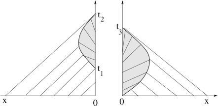
Figure 3: Left: an incoming road which is initially free. For $t_{1}<t<t_{2}$ part of the road is congested (shaded area). Right: an outgoing road which is initially congested. For $0<t<t_{3}$ part of the road is free (shaded area). In both cases, a shock marks the boundary between the free and the congested region.

The next lemma plays a key role in the proof of Theorem 2. It shows that, for any $t>0$, the maximum possible flux at the boundary of any incoming or outgoing road is greater or equal to the maximum flux computed at $t=0$. Lemma 1. Let $\rho_{k}=\rho_{k}(t,x)$, $k\in{\cal I}\cup{\cal O}$ be the solution of the Riemann problem with initial data (3.1). As in (2.9)-(2.10) call $\omega_{k}^{\diamondsuit}=\omega_{k}(\rho_{k}^{\diamondsuit})$ the maximum possible fluxes. Similarly, for $t>0$ call $\omega_{k}(t)=\omega_{k}(\bar{\rho}_{k}(t))$ the corresponding maximum fluxes. Then

$$\omega_{k}(t)~{}\in~{}\bigl{\{}\omega_{k}^{\diamondsuit},\,f_{k}^{max}\bigr{\}}\qquad\qquad\hbox{for all}~{}k\in{\cal I}\cup{\cal O},\quad t\geq 0.$$ (3.3)

Proof. 1. We first consider an incoming road $i\in{\cal I}$.

CASE 1: The road is initially congested, namely $\rho_{i}^{\diamondsuit}\geq\rho_{i}^{max}$. In this case the $i$-th road always remains congested and we have $\omega_{i}(t)=\omega_{i}^{\diamondsuit}=f_{i}^{max}$, for every $t\geq 0$.

CASE 2: The road is initially free, namely $\rho_{i}^{\diamondsuit}<\rho_{i}^{max}$. For a given $t>0$, two subcases may occur.

• There exists a characteristic with positive speed, reaching the point $(t,0)$. Since this characteristic must start at a point $x_{0}<0$, we conclude that $\rho_{i}(t,0-)=\rho_{i}(0,x_{0})=\rho_{i}^{\diamondsuit}$. Hence $\omega_{i}(t)=\omega_{i}^{\diamondsuit}$.

• There exists a neighborhood of $(t,0)$ covered with characteristics having negative speed. In this case $\rho_{i}(t,0-)\geq\rho_{i}^{max}$, hence $\omega_{i}(t)=f_{i}^{max}$.

2. For an outgoing road $j\in{\cal O}$, the analysis is similar.

CASE 1: The road is initially free, namely $\rho_{j}^{\diamondsuit}\leq\rho_{j}^{max}$. In this case the $j$-th road always remains free and we have $\omega_{j}(t)=\omega_{j}^{\diamondsuit}=f_{j}^{max}$, for every $t\geq 0$.

CASE 2: The road is initially congested, namely $\rho_{j}^{\diamondsuit}>\rho_{j}^{max}$. For a given $t>0$, two subcases may occur.

• There exists a characteristic with negative speed, reaching the point $(t,0)$. Since this characteristic must start at a point $x_{0}>0$, we conclude that $\rho_{j}(t,0+)=\rho_{j}(0,x_{0})=\rho_{j}^{\diamondsuit}$. Hence $\omega_{j}(t)=\omega_{j}^{\diamondsuit}$.

• There exists a neighborhood of $(t,0)$ covered with characteristics having positive speed. In this case $\rho_{j}(t,0+)\geq\rho_{j}^{max}$, hence $\omega_{j}(t)=f_{j}^{max}$.

MM     

4 Proof of Theorem 1

Let $\rho_{k}^{\diamondsuit}$, $k\in{\cal I}\cup{\cal O}$ be the initial densities of cars on the incoming and outgoing roads, and let $\theta_{ij}$ be the drivers’ turning preferences, as in (2.6). Call $\omega_{i}^{\diamondsuit},\omega_{j}^{\diamondsuit}$ the maximum possible boundary fluxes on the incoming and outgoing roads, and define $\bar{s}$ as in (2.16). Two cases will be considered, shown in Fig. 4. CASE 1: $\bar{s}=M$, so that $\gamma(\bar{s})~{}=~{}(\omega_{1}^{\diamondsuit},\omega_{2}^{\diamondsuit},\ldots,\omega_{m}^{\diamondsuit})$. This is the case where none of the incoming roads remains congested, and all the drivers arriving at the intersection can immediately proceed to the outgoing road of their choice.

In this case we choose the initial queues

$$q^{\diamondsuit}_{j}~{}=~{}0\qquad\qquad\hbox{for all}~{}~{}~{}j\in{\cal O}\,.$$

With these choices, the solution of the Cauchy problem with buffer coincides with the self-similar solution determined by the Limit Riemann Solver (LRS). The buffer remains always empty: $q_{j}(t)=0$ for all $t\geq 0$ and $j\in{\cal O}$. CASE 2: $\bar{s}<M$. In this case there exists an index $j^{*}\in{\cal O}$ such that

$$\sum_{i\in{\cal I}}\gamma_{i}(\bar{s})\theta_{ij^{*}}~{}=~{}\omega_{j^{*}}^{\diamondsuit}\,.$$ (4.1)

When this happens, the entire flow through the intersection is restricted by the number of cars that can exit toward the single congested road $j^{*}$. We then define

$$q^{*}~{}\doteq~{}M-\bar{s}\,,$$ (4.2)

and choose the initial queues to be

$$q_{j}^{\diamondsuit}~{}=~{}\left\{\begin{array}[]{cl}q^{*}&\hbox{if}~{}~{}~{}j=j^{*}\cr 0&\hbox{if}~{}~{}~{}j\not=j^{*}.\end{array}\right.$$ (4.3)

Then the corresponding solution coincides with the self-similar solution determined by the Limit Riemann Solver (LRS). Indeed, by the definition of $\gamma(\bar{s})$, for every $j\in{\cal O}$ we have

$$\sum_{i}\min\Big{\{}c_{i}(M-q^{*}),~{}\omega_{i}\Big{\}}\cdot\theta_{ij}~{}=~{}\sum_{i}\gamma_{i}(\bar{s})\,\theta_{ij}~{}\leq~{}\omega_{j}\,,$$ (4.4)

with equality holding when $j=j^{*}$. By (4.4), all queues remain constant in time, namely $q_{j^{*}}(t)=q^{*}$ and $q_{j}(t)=0$ for $j\not=j^{*}$.

MM     

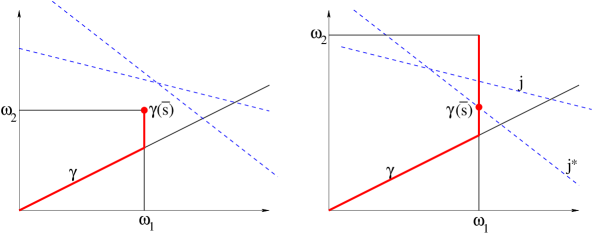
Figure 4: The two cases in the proof of Theorem 1. Left: none of the outgoing roads provides a restriction on the fluxes of the incoming roads. The queues are zero. Right: one of the outgoing roads is congested and restricts the maximum flux through the node.

Remark 2. In the proof of Theorem 1, the queue sizes $q_{j}^{\diamondsuit}$ may not be uniquely determined. Indeed, in Case 2 there may exist two distinct indices $j^{*}_{1},j^{*}_{2}\in{\cal O}$ such that

$$\sum_{i\in{\cal I}}\gamma_{i}(\bar{s})\theta_{ij_{1}^{*}}~{}=~{}\omega_{j_{1}^{*}}\,,\qquad\qquad\sum_{i\in{\cal I}}\gamma_{i}(\bar{s})\theta_{ij_{2}^{*}}~{}=~{}\omega_{j_{2}^{*}}\,.$$

When this happens, we can choose the queue sizes to be

$$q_{j}^{\diamondsuit}~{}=~{}\left\{\begin{array}[]{cl}\alpha q^{*}&\hbox{if}~{}~{}~{}j=j^{*}_{1}\,,\\[8.53581pt] (1-\alpha)q^{*}&\hbox{if}~{}~{}~{}j=j^{*}_{2}\,,\\[8.53581pt] 0&\hbox{if}~{}~{}~{}j\notin\{j^{*}_{1},j^{*}_{2}\},\end{array}\right.$$ (4.5)

for any choice of $\alpha\in[0,1]$.

5 Proof of Theorem 2

In this section we prove that, for any initial data, as $t\to+\infty$ the solution to the Riemann problem with buffer converges as to the self-similar function determined by the Limit Riemann Solver (LRS). The main argument can be divided in three main steps. (i) Establish an upper bound on the size $q=\sum_{j}q_{j}$ of the queue insider the buffer, showing that $\limsup_{t\to\infty}q(t)\leq M-\bar{s}$. (ii) Establish the lower bound $\liminf_{t\to\infty}q(t)\geq M-\bar{s}$. (iii) Using the previous steps, show that as $t\to\infty$ all boundary fluxes in the solution with buffer converge to the corresponding fluxes determined by (LRS). From this fact, the limit (2.22) follows easily. Given the densities $\rho_{i}^{\diamondsuit}$ on the incoming roads $i\in{\cal I}$, call $\omega^{\diamondsuit}_{i}$ the corresponding maximal flows, as in (2.9). Call $\hat{q}_{i}$ the value of the queue such that

$$c_{i}(M-\hat{q}_{i})~{}=~{}\omega_{i}^{\diamondsuit}\,.$$

Without loss of generality, we can assume

$$0~{}\leq~{}\hat{q}_{m}~{}\leq~{}\cdots~{}\leq~{}\hat{q}_{2}~{}\leq~{}\hat{q}_{1}\,.$$ (5.1)

At an intuitive level, we have

• If the queue inside the buffer is small, i.e. $q<\hat{q}_{i}$, then all drivers arriving from the $i$-th road can access the intersection, and the $i$-th road will become free.

• If the queue inside the buffer is large, i.e. $q>\hat{q}_{i}$, then not all drivers coming from the $i$-th road can immediately access the intersection, and the $i$-th road will become congested.

This can be formulated in a more precise way as follows. By the definition (2.16), if $q>M-\bar{s}$ one has

$$\sum_{i\in{\cal I}}\min\{c_{i}(M-q),~{}\omega_{i}^{\diamondsuit}\}\cdot\theta_{ij}~{}<~{}\omega_{j}^{\diamondsuit}\qquad\quad\hbox{for every}~{}~{}j\in{\cal O}\,.$$ (5.2)

On the other hand, if $q<M-\bar{s}$, let $j^{*}\in{\cal O}$ be an index such that (4.1) holds. We then have

$$\sum_{i\in{\cal I}}\min\{c_{i}(M-q),~{}\omega_{i}^{\diamondsuit}\}\cdot\theta_{ij^{*}}~{}>~{}\omega_{j^{*}}^{\diamondsuit}\,.$$ (5.3)

Figure 5: A case with three incoming roads. For large times, the first two roads become free, while the third road remains congested.

The proof is achieved in several steps. 1. We first study the case where, in the solution determined by the Limit Riemann Solver, at least one of the outgoing roads is congested (Fig. 4, right), so that (4.1) holds. Let $\bar{s}$ be as in (2.16). As in (4.2), define the asymptotic size of the queue to be $q^{*}=M-\bar{s}>0$. To fix the ideas, assume

$$0~{}\leq~{}\hat{q}_{m}~{}\leq~{}\cdots~{}\leq~{}\hat{q}_{\nu+1}~{}\leq~{}q^{*}~{}<~{}\hat{q}_{\nu}~{}\leq~{}\cdots~{}\leq~{}\hat{q}_{2}~{}\leq~{}\hat{q}_{1}\,.$$ (5.4)

In this setting, we will show that for $t$ large the incoming roads $i=1,\ldots,\nu$ will be free, while the incoming roads with $\hat{q}_{i}<q^{*}$ will be congested. More precisely, we shall prove the following

Claim. There exist times

$$0~{}=~{}t_{0}~{}=~{}\tau_{0}~{}<~{}t_{1}~{}<~{}\tau_{2}~{}<~{}t_{2}~{}<~{}\cdots~{}<\tau_{\nu}~{}<~{}t_{\nu}$$ (5.5)

and constants $\delta_{\ell},\varepsilon_{\ell}>0$, $\ell=1,\ldots,\nu$, with the following properties.

• If $t\geq t_{\ell-1}$, then we have the implication

  $$q(t)~{}\geq~{}\hat{q}_{\ell}-\delta_{\ell}\qquad\Longrightarrow\qquad\dot{q}(t)~{}\leq~{}-\varepsilon_{\ell}~{}<~{}0\,.$$ (5.6)

• If $t\geq\tau_{\ell}$, then $q(t)\leq\hat{q}_{\ell}-\delta_{\ell}$

• For all times $t\geq t_{\ell}$ the incoming road $\ell$ is free. Hence its flux near the intersection satisfies

  $$f_{\ell}(t)~{}=~{}\omega_{\ell}^{\diamondsuit}\qquad\qquad\hbox{for all}~{}t\geq t_{\ell}\,.$$ (5.7)

The above claim is proved by induction on $\ell=1,\ldots,\nu$.

We begin with $\ell=1$. For any $t\geq 0$, if $q(t)\geq\hat{q}_{1}$ then by (5.4) we have $q(t)>q^{*}$. Using Lemma 1, we thus obtain

$$\dot{q}_{j}(t)~{}\leq~{}\sum_{i}c_{i}(M-q(t))\theta_{ij}-\omega_{j}^{\diamondsuit}\qquad\qquad\hbox{if}~{}~{}q_{j}(t)>0.$$

Therefore, if $q_{j}(t)>0$, then

$$\dot{q}_{j}(t)~{}\leq~{}-2\varepsilon_{1j}~{}<~{}0$$

for some $\varepsilon_{1j}>0$. By continuity, there exists $\delta_{1}>0$ such that

$$q(t)>\hat{q}_{1}-\delta_{1}\,,\qquad q_{j}(t)>0\qquad\Longrightarrow\qquad\dot{q}_{j}(t)~{}\leq~{}-\varepsilon_{1j}\,.$$ (5.8)

We observe that, if $q(t)>\hat{q}_{1}-\delta_{1}>0$, then $q_{j}(t)>0$ for some $j\in{\cal O}$. Setting $\varepsilon_{1}\doteq\min_{j}\varepsilon_{1j}$, we obtain (5.6) for $\ell=1$.

From the implication

$$q(t)~{}\geq~{}\hat{q}_{1}-\delta_{1}\qquad\Longrightarrow\qquad\dot{q}(t)~{}\leq~{}-\varepsilon_{1}\,,$$

it follows $q(t)\leq\hat{q}_{1}-\delta_{1}$ for all $t\geq\tau_{1}$ sufficiently large. This yields (ii), for $\ell=1$.

Next, for $t>\tau_{1}$, the flux of cars arriving to the intersection from road 1 is

$$f_{1}(t)~{}=~{}\min\{\omega_{1}^{\diamondsuit}\,,~{}c_{1}(M-q(t))\}$$

If road 1 is congested near the intersection, then for $t>\tau_{1}$ the outgoing flux is

$$f_{1}(t)~{}=~{}c_{1}(M-q(t))~{}\geq~{}c_{1}(M-\hat{q}_{1}+\delta_{1})\}~{}=~{}\omega_{1}^{\diamondsuit}-\delta_{1}^{\prime}\,,$$

for some $\delta_{1}^{\prime}>0$. As a consequence, road 1 must become free within time

$$t_{1}~{}=~{}\tau_{1}+{1\over\delta_{1}^{\prime}}\cdot\int_{0}^{\tau_{1}}[\omega_{1}^{\diamondsuit}-f_{1}(t)]\,dt\,.$$

This proves (iii), in the case $\ell=1$. The general inductive step is very similar. Assume that the statements (i)–(iii) have been proved for $\ell-1$. Then for $t\geq t_{\ell-1}$ the incoming roads $i=1,\ldots,\ell-1$ are free. The flux of cars reaching the intersection from these roads is $f_{i}(t)=\omega_{i}^{\diamondsuit}$.

Now assume that $t>t_{\ell-1}$ and $q(t)\geq\hat{q}_{\ell}$. In this case, $q(t)\geq\hat{q}_{i}$ for all $i\in{\cal I}$, $i\geq\ell$. Using Lemma 1, for any $j\in{\cal O}$ we thus obtain

$$\dot{q}_{j}(t)~{}\leq~{}\sum_{i<\ell}\omega_{i}^{\diamondsuit}\theta_{ij}+\sum_{i\geq\ell}c_{i}(M-q(t))\theta_{ij}-\omega_{j}^{\diamondsuit}\qquad\qquad\hbox{if}~{}~{}q_{j}(t)>0.$$

Therefore, if $q_{j}(t)>0$, then

$$\dot{q}_{j}(t)~{}\leq~{}-2\varepsilon_{\ell j}~{}<~{}0$$

for some constants $\varepsilon_{\ell j}$. By continuity, there exists $\delta_{\ell}>0$ such that

$$q(t)>\hat{q}_{\ell}-\delta_{\ell}\,,\qquad q_{j}(t)>0\qquad\Longrightarrow\qquad\dot{q}_{j}(t)~{}\leq~{}-\varepsilon_{\ell j}\,.$$ (5.9)

Setting $\varepsilon_{\ell}\doteq\min_{j}\varepsilon_{\ell j}$, we obtain (5.6).

From the implication

$$q(t)~{}\geq~{}\hat{q}_{\ell}-\delta_{\ell}\qquad\Longrightarrow\qquad\dot{q}(t)~{}\leq~{}-\varepsilon_{\ell}\,,$$

it follows $q(t)\leq\hat{q}_{\ell}-\delta_{\ell}$ for all $t\geq\tau_{\ell}$ sufficiently large. This yields (ii).

Finally, for $t>\tau_{\ell}$, the flux of cars arriving to the intersection from road $\ell$ is

$$f_{\ell}(t)~{}=~{}\min\{\omega_{\ell}^{\diamondsuit}\,,~{}c_{\ell}(M-q(t))\}$$

If road $\ell$ is congested near the intersection, then for $t>\tau_{\ell}$ the outgoing flux is

$$f_{\ell}(t)~{}=~{}c_{\ell}(M-q(t))~{}\geq~{}c_{\ell}(M-\hat{q}_{\ell}+\delta_{\ell})\}~{}=~{}\omega_{\ell}^{\diamondsuit}-\delta_{\ell}^{\prime}\,,$$

for some $\delta_{\ell}^{\prime}>0$. As a consequence, road $\ell$ must become free within time

$$t_{\ell}~{}=~{}\tau_{\ell}+{1\over\delta_{\ell}^{\prime}}\cdot\int_{0}^{\tau_{\ell}}[\omega_{\ell}^{\diamondsuit}-f_{\ell}(t)]\,dt\,.$$

This proves (iii). By induction on $\ell$, our claim is proved. 2. We now prove that, for any $\varepsilon>0$, there exists a time $t_{\varepsilon}>t_{\nu}$ large enough so that

$$q(t)~{}\leq~{}q^{*}+\varepsilon\qquad\qquad\hbox{for all}~{}t~{}\geq~{}t_{\varepsilon}\,.$$ (5.10)

Indeed, if $t>t_{\ell}$ , then the same arguments used before yield the implication

$$q(t)~{}\geq~{}q^{*}+\varepsilon\qquad\Longrightarrow\qquad\dot{q}(t)~{}\leq~{}-\delta~{}<~{}0,$$

for some $\delta=\delta(\varepsilon)>0$. Hence, $q(t)\leq q^{*}+\varepsilon$ whenever

$$t~{}\geq~{}t_{\varepsilon}~{}=~{}t_{\nu}+\delta^{-1}q(t_{\nu}).$$

3. In this step we prove a lower bound on the queue. Namely, for any $\varepsilon^{\sharp}>0$ there exists a time $t^{\sharp}>0$ such that

$$q(t)~{}\geq~{}q^{*}-\varepsilon^{\sharp}\qquad\qquad\hbox{for all}~{}t~{}\geq~{}t^{\sharp}\,.$$ (5.11)

Toward this goal, choose $j^{*}\in{\cal O}$ such that (4.1) holds. Then

$$\dot{q}_{j^{*}}(t)~{}=~{}\sum_{i}\min\bigl{\{}c_{i}(M-q(t)),\,\omega_{i}(\bar{\rho}(t))\bigr{\}}\theta_{ij}-\bar{f}_{j^{*}}(t).$$

Now assume $q(t)<q^{*}-\varepsilon^{\sharp}$. If road $j^{*}$ is initially free, then it remains free for all times $t\geq 0$. Hence $f_{j^{*}}(t)\leq f_{j}^{max}=\omega_{j}^{\diamondsuit}$. In this case we have

$$\dot{q}_{j^{*}}(t)~{}\geq~{}\sum_{i}\min\bigl{\{}c_{i}(M-q^{*}+\varepsilon^{\sharp}),~{}\omega_{i}^{\diamondsuit}\bigr{\}}\theta_{ij}-\omega_{j^{*}}^{\diamondsuit}~{}\geq~{}\delta^{\sharp}$$

for some $\delta^{\sharp}~{}>~{}0$. Therefore (5.11) holds with

$$t^{\sharp}~{}\doteq~{}{q_{j^{*}}(0)-q^{*}+\varepsilon^{\sharp}\over\delta^{\sharp}}\,.$$

Next, we consider the more difficult case where the outgoing road $j^{*}$ is initially congested. We claim that, if $q(\tau)\leq q^{*}$ at some time $\tau\geq t_{\nu}$, then $q(t)\leq q^{*}$ for all $t\geq\tau$. Indeed, for any $j\in{\cal O}$, if $q_{j}(t)>0$, then

$$\dot{q}_{j}(t)~{}\leq~{}\sum_{i\leq\nu}\omega_{i}^{\diamondsuit}\theta_{ij}+\sum_{i>\nu}c_{i}(M-q(t))\theta_{ij}-\omega_{j}^{\diamondsuit}\,.$$ (5.12)

Observing that the right hand side of (5.12) is nonpositive when $q(t)=q^{*}$, our claim is proved.

Now call

$$E_{j^{*}}(t)~{}\doteq~{}\omega_{j^{*}}^{\diamondsuit}\,t-\int_{0}^{t}\bar{f}_{j^{*}}(s)\,ds\,,$$

and observe that $E_{j^{*}}(t)\geq 0$ for all $t$, while

$$q(t)~{}\leq~{}q^{*}\qquad\Longrightarrow\qquad\dot{E}_{j^{*}}(t)~{}\leq~{}0.$$ (5.13)

For $t>t_{\nu}$ we have

$$\dot{q}_{j^{*}}(t)-\dot{E}_{j^{*}}(t)~{}\geq~{}\sum_{i\leq\nu}\omega_{i}^{\diamondsuit}\theta_{ij^{*}}+\sum_{i>\nu}\min\left\{c_{i}(M-q(t)),~{}\omega_{i}^{\diamondsuit}\right\}\theta_{ij^{*}}-\omega_{j^{*}}^{\diamondsuit}\,.$$ (5.14)

If $q(t)\leq q^{*}-\varepsilon^{\sharp}$, then

$$\dot{q}_{j^{*}}(t)-\dot{E}_{j^{*}}(t)~{}\geq~{}\delta^{\sharp}$$ (5.15)

for some $\delta^{\sharp}>0$.

Finally, assume that $q(\tau)<q^{*}-\varepsilon^{\sharp}$, for some $\tau\geq t_{\nu}$. Then (5.13) and (5.15) imply (5.11), with

$$t^{\sharp}~{}=~{}\tau+{E_{j^{*}}(\tau)+q^{*}-q(\tau)\over\delta^{\sharp}}\,.$$

4. Denote by $\rho_{k}(t,x)$, $k\in{\cal I}\cup{\cal O}$, the solution to the Riemann problem with buffer, and $\sigma_{k}(t,x)$ the self-similar solution determined by the Limit Riemann Solver (LRS). From the limit $\lim_{t\to\infty}q(t)=q^{*}$ proved in the previous steps, it follows that all boundary fluxes $f_{k}(t)$ converge to the corresponding boundary fluxes $\bar{f}_{k}$ in the self-similar solution determined by (LRS).

Now consider an incoming road $i\in{\cal I}$. Since the initial data coincide

$$\rho_{i}(0,x)~{}=~{}\sigma_{i}(0,x)~{}=~{}\rho_{i}^{\diamondsuit}\qquad\qquad x<0\,,$$

for every $t>0$ by [11] we have the estimate

$$\int_{-\infty}^{0}\bigl{|}\rho_{i}(t,x)-\sigma_{i}(t,x)\bigr{|}\,dx~{}\leq~{}\int_{0}^{t}|f_{i}(s)-\bar{f}_{i}|\,ds\,.$$ (5.16)

From the limit

$$\lim_{t\to\infty}|f_{i}(t)-\bar{f}_{i}|~{}=~{}0$$

it thus follows

$$\lim_{t\to\infty}{1\over t}\int_{-\infty}^{0}\bigl{|}\rho_{i}(t,x)-\sigma_{i}(t,x)\bigr{|}\,dx~{}=~{}0.$$

For outgoing roads $j\in{\cal O}$, the estimates are entirely similar. This achieves a proof of Theorem 2 in the case where (4.1) holds for some $j^{*}\in{\cal O}$. 5. It remains to consider the case (Fig. 4, left) where

$$\sum_{i}\omega_{i}^{\diamondsuit}\theta_{ij}~{}<~{}\omega_{j}^{\diamondsuit}$$ (5.17)

for every $j\in{\cal O}$. In this case, the arguments in step 1 show that, for all $t\geq t_{m}$ sufficiently large, all incoming roads become free. In this case, for all times $t\geq t^{\sharp}$ sufficiently large the incoming fluxes are

$$f_{i}(t)~{}=~{}\omega_{i}^{\diamondsuit}~{}=~{}\bar{f}_{i}\,.\qquad\qquad i\in{\cal I}.$$

Moreover, for $t$ large all queue sizes become $q_{j}(t)=0$, and the outgoing fluxes are

$$f_{j}(t)~{}=~{}\sum_{i}\omega_{i}^{\diamondsuit}\theta_{ij}~{}=~{}\bar{f}_{j}\qquad\qquad j\in{\cal O}.$$

Inserting these identities in (5.16), we conclude the proof as in the previous case. MM     

Acknowledgment. The first author was partially supported by NSF, with grant DMS-1411786: “Hyperbolic Conservation Laws and Applications”. The second author recieved financial support for a stay at Penn State University from Tandberg radiofabrikks fond, Norges tekniske høgskoles fond, and Generaldirektør Rolf Ostbyes stipendfond ved NTNU.

References

[1] A. Bressan, S. Canic, M. Garavello, M. Herty, and B. Piccoli,
Flow on networks: recent results and perspectives,
EMS Surv. Math. Sci.1 (2014), 47–111.
[2] A. Bressan and K. Nguyen,
Conservation law models for traffic flow on a network of roads.
Netw. Heter. Media10 (2015), 255–293.
[3] A. Bressan and F. Yu,
Continuous Riemann solvers for traffic flow at a junction.
Discr. Cont. Dyn. Syst.35 (2015), 4149–4171.
[4] G. M. Coclite, M. Garavello, and B. Piccoli,
Traffic flow on a road network.
SIAM J. Math. Anal.36 (2005), 1862–1886.
[5] M. Garavello, Conservation laws at a node.
Nonlinear Conservation Laws and Applications,
The IMA Volumes in Mathematics and its Applications, Vol. 15.
A. Bressan, G. Q. Chen, M. Lewicka,
and D. Wang Editors, 2011, pp. 293–302.
[6]
M. Garavello and B. Piccoli, Traffic Flow on
Networks. Conservation Laws Models.
AIMS Series on Applied Mathematics, Springfield, Mo., 2006.
[7]
M. Garavello and B. Piccoli,
Conservation laws on complex networks.
Ann. Inst. H. Poincaré26 (2009) 1925–1951.
[8] M. Herty, J. P. Lebacque, and S. Moutari,
A novel model for intersections of vehicular traffic flow.
Netw. Heterog. Media4 (2009), 813–826.
[9]
H. Holden and N. H. Risebro. A mathematical model of traffic flow on a network
of unidirectional roads. SIAM J. Math. Anal.26 (1995), 999–1017.
[10] C. Imbert, R. Monneau, and H. Zidani, A Hamilton-Jacobi approach
to junction problems and application to traffic flows.
ESAIM-COCV19 (2013), 129–166.
[11] P. Le Floch,
Explicit formula for scalar non-linear conservation laws with boundary condition.
Math. Methods Appl. Sciences10 (1988), 265–287.
[12]
M. Lighthill and G. Whitham, On kinematic waves. II.
A theory of traffic flow on long crowded roads.
Proceedings of the Royal Society of London: Series A,229 (1955), 317–345.
[13]
P. I. Richards, Shock waves on the highway,
Oper. Res.4
(1956), 42-51.