Structured Compressive Sensing Based Spatio-Temporal
Joint Channel Estimation for FDD Massive MIMO

Abstract

Massive MIMO is a promising technique for future 5G communications due to its high spectrum and energy efficiency. To realize its potential performance gain, accurate channel estimation is essential. However, due to massive number of antennas at the base station (BS), the pilot overhead required by conventional channel estimation schemes will be unaffordable, especially for frequency division duplex (FDD) massive MIMO. To overcome this problem, we propose a structured compressive sensing (SCS)-based spatio-temporal joint channel estimation scheme to reduce the required pilot overhead, whereby the spatio-temporal common sparsity of delay-domain MIMO channels is leveraged. Particularly, we first propose the non-orthogonal pilots at the BS under the framework of CS theory to reduce the required pilot overhead. Then, an adaptive structured subspace pursuit (ASSP) algorithm at the user is proposed to jointly estimate channels associated with multiple OFDM symbols from the limited number of pilots, whereby the spatio-temporal common sparsity of MIMO channels is exploited to improve the channel estimation accuracy. Moreover, by exploiting the temporal channel correlation, we propose a space-time adaptive pilot scheme to further reduce the pilot overhead. Additionally, we discuss the proposed channel estimation scheme in multi-cell scenario. Simulation results demonstrate that the proposed scheme can accurately estimate channels with the reduced pilot overhead, and it is capable of approaching the optimal oracle least squares estimator.

I Introduction

Massive MIMO employing a large number of antennas at the base station (BS) to simultaneously serve multiple users, has recently emerged as a promising approach to realize high-throughput green wireless communications [1]. By exploiting the large number of degrees of spatial freedom, massive MIMO can boost the system capacity and energy efficiency by orders of magnitude. Therefore, massive MIMO has been widely recognized as a key enabling technique for future spectrum and energy efficient 5G communications [2].

In massive MIMO systems, an accurate acquisition of the channel state information (CSI) is essential for signal detection, beamforming, resource allocation, etc. However, due to massive antennas at the BS, each user has to estimate channels associated with hundreds of transmit antennas, which results in the prohibitively high pilot overhead. Hence, how to realize the accurate channel estimation with the affordable pilot overhead becomes a challenging problem, especially for frequency division duplex (FDD) massive MIMO systems [3]. To date, most of researches on massive MIMO sidestep this challenge by assuming the time division duplex (TDD) protocol, where the CSI in the uplink can be more easily acquired at the BS due to the small number of single-antenna users and the powerful processing capability of the BS, and then the channel reciprocity property can be leveraged to directly obtain the CSI in the downlink [4]. However, due to the calibration error of radio frequency chains and limited coherence time, the CSI acquired in the uplink may not be accurate for the downlink [5, 6]. More importantly, compared with TDD systems, FDD systems can provide more efficient communications with low latency [7], and it has dominated current cellular systems. Therefore, it is of importance to explore the challenging problem of channel estimation for FDD massive MIMO systems, which can facilitate massive MIMO to be backward compatible with current FDD dominated cellular networks.

Recently, there have been extensive studies on channel estimation for conventional small-scale FDD MIMO systems [10, 11, 13, 8, 9, 12, 14]. It has been proven that the equi-spaced and equi-power orthogonal pilots can be optimal to estimate the non-correlated Rayleigh MIMO channels for one OFDM symbol, where the required pilot overhead increases with the number of transmit antennas [8]. By exploiting the spatial correlation of MIMO channels, the pilot overhead to estimate Rician MIMO channels can be reduced [9]. Furthermore, by exploiting the temporal channel correlation, further reduced pilot overhead can be achieved to estimate MIMO channels associated with multiple OFDM symbols [10, 11]. Currently, orthogonal pilots have been widely used in the existing MIMO systems, where the pilot overhead is not a big issue due to the small number of transmit antennas (e.g., up to eight antennas in LTE-Advanced system) [13, 12, 14]. However, this issue can be critical in massive MIMO systems due to massive number of antennas at the BS (e.g., 128 antennas or even more at the BS [2]).

In [15], an approach to exploit the temporal correlation and sparsity of delay-domain channels for the reduced pilot overhead has been proposed for FDD massive MIMO systems, but the interference cancellation of training sequences of different transmit antennas will be difficult when the number of transmit antennas is large. [17, 18, 16] leveraged the spatial correlation and sparsity of delay-domain MIMO channels to estimate channels with the reduced pilot overhead, but the assumption of the known channel sparsity level at the user is unrealistic. By exploiting the spatial channel correlation, the compressive sensing (CS)-based channel estimation schemes were proposed in [19, 20, 21], but the leveraged spatial correlation can be impaired due to the non-ideal antenna array [3, 5]. [22] proposed an open-loop and closed-loop channel estimation scheme for massive MIMO, but the long-term channel statistics perfectly known at the user can be difficult.

On the other hand, for typical broadband wireless communication systems, delay-domain channels intrinsically exhibit the sparse nature due to the limited number of significant scatterers in the propagation environments and large channel delay spread [23, 24, 15, 26, 29, 28, 27, 25]. Meanwhile, for MIMO systems with co-located antenna array at the BS, channels between one user and different transmit antennas at the BS exhibit very similar path delays due to very similar scatterers in the propagation environments, which indicates that delay-domain channels between the user and different transmit antennas at the BS share the common sparsity when the aperture of the antenna array is not very large [3, 30]. Moreover, since the path delays vary much slower than the path gains due to the temporal channel correlation, such sparsity is almost unchanged during the coherence time [31]. In this paper, such channel properties of MIMO channels are referred to as the spatio-temporal common sparsity, which is usually not considered in most of current work.

In this paper, by exploiting the spatio-temporal common sparsity of delay-domain MIMO channels, we propose a structured compressive sensing (SCS)-based spatio-temporal joint channel estimation scheme with significantly reduced pilot overhead for FDD massive MIMO systems. Specifically, at the BS, we propose a non-orthogonal pilot scheme under the framework of CS theory, which is essentially different from the widely used orthogonal pilots under the framework of classical Nyquist sampling theorem. Compared with conventional orthogonal pilots, the proposed non-orthogonal pilot scheme can substantially reduce the required pilot overhead for channel estimation. At the user side, we propose an adaptive structured subspace pursuit (ASSP) algorithm for channel estimation, whereby the spatio-temporal common sparsity of delay-domain MIMO channels is leveraged to improve the channel estimation performance from the limited number of pilots. Furthermore, by leveraging the temporal channel correlation, we propose a space-time adaptive pilot scheme to realize the accurate channel estimation with further reduced pilot overhead, where the specific pilot signals should consider the geometry of antenna array at the BS and the mobility of served users. Additionally, we further extend the proposed channel estimation scheme from the single-cell scenario to the multi-cell scenario. Finally, simulation results verify that the proposed scheme outperforms its conventional counterparts with reduced pilot overhead, where the performance of the SCS-based channel estimation scheme approaches that of the oracle least squares (LS) estimator.

The rest of the paper is organized as follows. Section II illustrates the spatio-temporal common sparsity of delay-domain MIMO channels. In Section III, the proposed SCS-based spatio-temporal joint channel estimation scheme is discussed in detail. In Section IV, we provide the performance analysis. Section V shows the simulation results. Finally, Section VI concludes this paper.

Notation: Boldface lower and upper-case symbols represent column vectors and matrices, respectively. The operator $\circ$ represents the Hadamard product, $\lfloor\cdot\rfloor$ denotes the integer floor operator, and $\rm{diag}\{\bf{x}\}$ is a diagonal matrix with elements of $\mathbf{x}$ on its diagonal. The matrix inversion, transpose, and Hermitian transpose operations are denoted by $(\cdot)^{-1}$, $(\cdot)^{\rm{T}}$, and $(\cdot)^{\rm{H}}$, respectively, while $(\cdot)^{{\dagger}}$ denotes the Moore-Penrose matrix inversion. $|\cdot|_{c}$ denotes the cardinality of a set, the $l_{2}$-norm operation and Frobenius-norm operation are given by $\|\cdot\|_{2}$ and $\|\cdot\|_{F}$, respectively. ${\Omega^{c}}$ denotes the complementary set of the set $\Omega$. $\rm{Tr}\{\cdot\}$ is the trace of a matrix. $\left\langle\cdot,\cdot\right\rangle$ is the Frobenius inner product, and $\left\langle{{\bf{A}}{\rm{,}}{\bf{B}}}\right\rangle{\rm{=Tr\{}}{{\bf{A}}^{\rm{H}}}{\bf{B}}{\rm{\}}}$. Finally, $\mathbf{\Phi}^{(l)}$ denotes the $l$th column vector of the matrix $\mathbf{\Phi}$.

II Spatio-Temporal Common Sparsity of Delay-Domain

Extensive experimental studies have shown that wireless broadband channels exhibit the sparsity in the delay domain. This is caused by the fact that the number of multipath dominating the majority of channel energy is small due to the limited number of significant scatterers in the wireless signal propagation environments, while the channel delay spread can be large due to the large difference between the time of arrival (ToA) of the earliest multipath and the ToA of the latest multipath [23, 24, 15, 26, 29, 28, 27, 25]. Specifically, in the downlink, the delay-domain channel impulse response (CIR) between the $m$th transmit antenna at the BS and one user can be expressed as

$${{\bf{h}}_{m,r}}={\left[{{h_{m,r}}[1],{h_{m,r}}[2],\cdots,{h_{m,r}}[L]}\right]^{\rm{T}}},1\leq m\leq M,$$ (1)

where $r$ is the index of the OFDM symbol in the time domain, $L$ is the equivalent channel length, $D_{m,r}=\text{supp}\{{{\bf{h}}_{m,r}}\}=\left\{{l:\left|{{h_{m,r}}[l]}\right|>p_{\rm{th}}},1\leq l\leq L\right\}$ is the support set of ${{\bf{h}}_{m,r}}$, and $p_{\rm{th}}$ is the noise floor according to [32]. The sparsity level of wireless channels is denoted as ${P_{m,r}}=\left|{{D_{m,r}}}\right|_{c}$, and we have $P_{m,r}\ll L$ due to the sparse nature of delay-domain channels [23, 24, 15, 26].

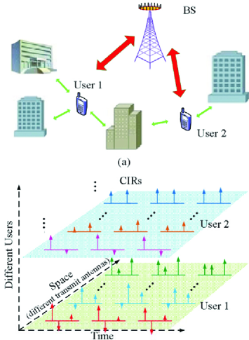
Figure 1: Spatio-temporal common sparsity of delay-domain MIMO channels: (a) Wireless channels exhibit the sparse nature due to the limited number of scatterers; (b) Delay-domain MIMO channels between the co-located antenna array and one user exhibit the spatio-temporal common sparsity.

Moreover, there are measurements showing that CIRs between different transmit antennas and one user exhibit very similar path delays [3, 30]. The reason is that, in typical massive MIMO geometry, the scale of the compact antenna array at the BS is relatively small compared with the large signal transmission distance, and channels associated with different transmit-receive antenna pairs share the common scatterers. Therefore, the sparsity patterns of CIRs of different transmit-receive antenna pairs have a large overlap. Moreover, for MIMO systems with not very large $M$, these CIRs can share the common sparse pattern [17, 3, 30], i.e.,

$$D_{1,r}=D_{2,r}=\cdots=D_{M,r},$$ (2)

which is referred to as the spatial common sparsity of wireless MIMO channels. For example, we consider the LTE-Advanced system working at a carrier frequency of $f_{c}=2~{}\rm{GHz}$ with a signal bandwidth of $f_{s}=10~{}\rm{MHz}$, and the uniform linear array (ULA) with the antenna spacing of half-wavelength. For two transmit antennas with the distance of 8 half-wavelengths, their maximum difference of path delays from the common scatterer is $\frac{{{8\lambda}/2}}{{{c}}}=4/f_{c}=0.002~{}\mu s$, which is negligible compared with the system sample period $T_{s}=1/f_{s}=0.1~{}\mu s$, where $\lambda$ and $c$ are the wavelength and the velocity of light, respectively. It should be pointed out that the path gains of different transmit-receive antenna pairs from the same scatterer can be different or even uncorrelated due to the non-isotropic antennas [5].

Finally, practical wireless channels also exhibit the temporal correlation even in fast time-varying scenarios [31]. It has been demonstrated that the path delays usually vary much slower than the path gains [31]. In other words, although the path gains can vary significantly from one OFDM symbol to another, the path delays remain almost unchanged during several successive OFDM symbols. This is due to the fact that the coherence time of path gains over time-varying channels is inversely proportional to the system carrier frequency, while the duration for path delay variation is inversely proportional to the system bandwidth [31]. For example, in the LTE-Advanced system with $f_{c}=2~{}\rm{GHz}$ and $f_{s}=10~{}\rm{MHz}$, the path delays vary at a rate that is about several hundred times slower than that of the path gains [15]. That is to say, during the coherence time of path delays, CIRs associated with $R$ successive OFDM symbols have the common sparsity due to the almost unchanged path delays, i.e.,

$$D_{m,r}=D_{m,r+1}=\cdots=D_{m,r+R-1},1\leq m\leq M.$$ (3)

This temporal correlation of wireless channels is also referred to as the temporal common sparsity of wireless channels in this paper.

The spatial and temporal channel correlations discussed above are jointly referred to as the spatio-temporal common sparsity of delay-domain MIMO channels, which can be illustrated in Fig. 1. This channel property is usually not considered in existing channel estimation schemes. In this paper, we will exploit this channel property to overcome the challenging problem of channel estimation for FDD massive MIMO.

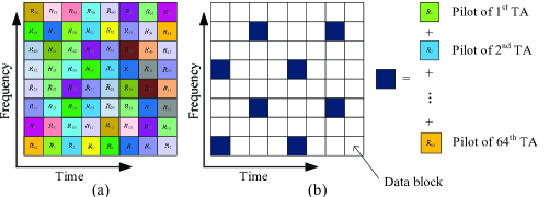
Figure 2: Pilot designs for massive MIMO with $M=64$ in one time-frequency resource block. (a) Conventional orthogonal pilot design; (b) Proposed non-orthogonal pilot design.

III Proposed SCS-Based Spatio-Temporal Joint Channel Estimation Scheme

In this section, the SCS-based spatio-temporal joint channel estimation scheme is proposed for FDD massive MIMO. First, we propose the non-orthogonal pilot scheme at the BS to reduce the pilot overhead. Then, we propose the ASSP algorithm at the user for reliable channel estimation. Moreover, we propose the space-time adaptive pilot scheme for further reduction of the pilot overhead. Finally, we briefly discuss the proposed channel estimation scheme extended to multi-cell scenario.

III-A Non-Orthogonal Pilot Scheme at the BS

The design of conventional orthogonal pilots is based on the framework of classical Nyquist sampling theorem, and this design has been widely used in the existing MIMO systems. The orthogonal pilots can be illustrated in Fig. 2 (a), where pilots associated with different transmit antennas occupy the different subcarriers. For massive MIMO systems with hundreds of transmit antennas, such orthogonal pilots will suffer from the prohibitively high pilot overhead.

In contrast, the design of the proposed non-orthogonal pilot scheme, as shown in Fig. 2 (b), is based on CS theory, and it allows pilots of different transmit antennas to occupy the completely same subcarriers. By leveraging the sparse nature of channels, the pilots used for channel estimation can be reduced substantially.

For the proposed non-orthogonal pilot scheme, we first consider the MIMO channel estimation for one OFDM symbol as an example. Particularly, we denote the index set of subcarriers allocated to pilots as $\xi$, which is uniquely selected from the set of $\left\{{1,2,\cdots,N}\right\}$ and identical for all transmit antennas. Here ${N_{p}}=\left|\xi\right|_{c}$ is the number of pilot subcarriers in one OFDM symbol, and $N$ is the number of subcarriers in one OFDM symbol. Moreover, we denote the pilot sequence of the $m$th transmit antenna as ${{\bf{p}}_{m}}\in\mathbb{C}^{N_{p}\times 1}$. The specific pilot design $\xi$ and $\left\{{{{\bf{p}}_{m}}}\right\}_{m=1}^{M}$ will be detailed in Section IV-A .

III-B SCS-Based Channel Estimation at the User

At the user, after the removal of the guard interval and discrete Fourier transformation (DFT), the received pilot sequence ${{\bf{y}}_{r}}\in\mathbb{C}^{N_{p}\times 1}$ of the $r$th OFDM symbol can be expressed as

$$\begin{array}[]{l}{{\bf{y}}}_{r}=\sum\limits_{m=1}^{M}{{\rm{diag}}\{{{\bf{p}}_{m}}\}{{\left.{\bf{F}}\right|}_{\xi}}\left[{\begin{array}[]{*{20}{l}}{{{\bf{h}}_{m,r}}}\\ {{{\bf{0}}_{(N-L)\times 1}}}\end{array}}\right]}+{\bf{w}}_{r}\\ ~{}~{}~{}=\sum\limits_{m=1}^{M}{{{\bf{P}}_{m}}{{\left.{{{\bf{F}}_{L}}}\right|}_{\xi}}{{\bf{h}}_{m,r}}}+{\bf{w}}_{r}=\sum\limits_{m=1}^{M}{{\bf{\Phi}}_{m}{{\bf{h}}_{m,r}}}+{\bf{w}}_{r},\end{array}$$ (4)

where ${{\bf{P}}_{m}}{\rm{=diag}}\{{{\bf{p}}_{m}}\}$, ${\bf{F}}\in\mathbb{C}^{N\times N}$ is a DFT matrix, ${{\bf{F}}_{L}}\in\mathbb{C}^{N\times L}$ is a partial DFT matrix consisted of the first $L$ columns of ${\bf{F}}$, ${\left.{{{\bf{F}}}}\right|_{\xi}}\in\mathbb{C}^{N_{p}\times N}$ and ${\left.{{{\bf{F}}_{L}}}\right|_{\xi}}\in\mathbb{C}^{N_{p}\times L}$ are the sub-matrices by selecting the rows of ${{{\bf{F}}}}$ and ${{{\bf{F}}_{L}}}$ according to $\xi$, respectively, ${\bf{w}}_{r}\in\mathbb{C}^{N_{p}\times 1}$ is the additive white Gaussian noise (AWGN) vector in the $r$th OFDM symbol, and ${{\bf{\Phi}}_{m}}={{\bf{P}}_{m}}{\left.{{{\bf{F}}_{L}}}\right|_{\xi}}$. Moreover, (4) can be rewritten in a more compact form as

$${\bf{y}}_{r}={{\bf{\Phi}}{\bf{\tilde{h}}}_{r}}+{\bf{w}}_{r},$$ (5)

where ${\bf{\Phi}}=\left[{{{\bf{\Phi}}_{1}},{{\bf{\Phi}}_{2}},\cdots,{{\bf{\Phi}}_{M}}}\right]\in\mathbb{C}^{{N_{p}}\times ML}$, and ${\bf{\tilde{h}}}_{r}={[{\bf{h}}_{1,r}^{\rm{T}},{\bf{h}}_{2,r}^{\rm{T}},\cdots,{\bf{h}}_{M,r}^{\rm{T}}]^{\rm{T}}}\in\mathbb{C}^{ML\times 1}$ is an aggregate CIR vector.

For massive MIMO systems, we usually have ${N_{p}}\ll ML$ due to the large number of transmit antennas $M$ and the limited number of pilots $N_{p}$. This indicates that we cannot reliably estimate ${\bf{\tilde{h}}}_{r}$ from ${\bf{y}}_{r}$ using conventional channel estimation schemes, since (5) is an under-determined system. However, the observation that ${\bf{\tilde{h}}}_{r}$ is a sparse signal due to the sparsity of $\{{{\bf{h}}_{m,r}}\}_{m=1}^{M}$ inspires us to estimate the sparse signal ${\bf{\tilde{h}}}_{r}$ of high dimension from the received pilot sequence ${\bf{y}}_{r}$ of low dimension under the framework of CS theory [33]. Moreover, the inherently spatial common sparsity of wireless MIMO channels can be also exploited for performance enhancement. Specifically, we rearrange the aggregate CIR vector ${\bf{\tilde{h}}}_{r}$ to obtain the equivalent CIR vector ${\bf{\tilde{d}}}_{r}$ as

$${{\bf{\tilde{d}}}}_{r}={[{\bf{d}}_{1,r}^{\rm{T}},{\bf{d}}_{2,r}^{\rm{T}},\cdots,{\bf{d}}_{L,r}^{\rm{T}}]^{\rm{T}}}\in\mathbb{C}^{{ML}\times 1},$$ (6)

where ${\bf{d}}_{l,r}=\left[{{h_{1,r}}[l],{h_{2,r}}[l],\cdots,{h_{M,r}}[l]}\right]^{\rm{T}}$ for $1\leq l\leq L$. Similarly, ${\bf{\Phi}}$ can be rearranged as ${\bf{\Psi}}$, i.e.,

$${\bf{\Psi}}=\left[{{{\bf{\Psi}}_{1}},{{\bf{\Psi}}_{2}},\cdots,{{\bf{\Psi}}_{L}}}\right]\in\mathbb{C}^{{N_{p}}\times ML},$$ (7)

where ${{\bf{\Psi}}_{l}}=\left[{{{{{{\bf{\Phi}}_{1}^{(l)}}}}},{{{{{\bf{\Phi}}_{2}^{(l)}}}}},\cdots,{{{{{\bf{\Phi}}_{M}^{(l)}}}}}}\right]=\left[{{{\bm{\psi}}_{1,l}},{{\bm{\psi}}_{2,l}},\cdots,{{\bm{\psi}}_{M,l}}}\right]\in\mathbb{C}^{{N_{p}}\times M}$. In this way, (5) can be reformulated as

$${{\bf{y}}}_{r}={\bf{\Psi}}{{\bf{\tilde{d}}}}_{r}+{{\bf{w}}}_{r}.\vspace*{-2.0mm}$$ (8)

From (8), it can be observed that due to the spatial common sparsity of wireless MIMO channels, the equivalent CIR vector ${\bf{\tilde{d}}}_{r}$ exhibits the structured sparsity [33].

Furthermore, the temporal correlation of wireless channels indicates that such spatial common sparsity in MIMO systems remains virtually unchanged over $R$ successive OFDM symbols, where $R$ is determined by the coherence time of the path delays [15]. Hence, wireless MIMO channels exhibit the spatio-temporal common sparsity during $R$ successive OFDM symbols. Considering (8) during $R$ adjacent OFDM symbols with the same pilot pattern, we have

$${\bf{Y}}={\bf{\Psi D}}+{\bf{W}},\vspace*{-2.0mm}$$ (9)

where ${\bf{Y}}\!=\!\left[{{{\bf{y}}_{r}},\!{{\bf{y}}_{r+1}},\!\cdots\!,\!{{\bf{y}}_{r+R-1}}}\right]\!\in\!\mathbb{C}^{N_{p}\times R}$ is the measurement matrix, ${\bf{D}}\!=\!\left[{{{{\bf{\tilde{d}}}}_{r}},\!{{{\bf{\tilde{d}}}}_{r+1}},\!\cdots\!,\!{{{\bf{\tilde{d}}}}_{r+R-1}}}\right]\!\in\!\mathbb{C}^{ML\times R}$ is the equivalent CIR matrix, and ${\bf{W}}=\left[{{{\bf{w}}_{r}},{{\bf{w}}_{r+1}},\cdots,{{\bf{w}}_{r+R-1}}}\right]\in\mathbb{C}^{N_{p}\times R}$ is the AWGN matrix. It should be pointed out that ${\bf{D}}$ can be expressed as

$${\bf{D}}={\rm{}}{[{\bf{D}}_{1}^{\rm{T}},{\bf{D}}_{2}^{\rm{T}},\cdots,{\bf{D}}_{L}^{\rm{T}}]^{\rm{T}}},\vspace*{-2.0mm}$$ (10)

where ${{{\bf{D}}_{l}}}$ for $1\leq l\leq L$ has the size of $M\times R$, and the $m$th row and $r$th column element of ${{{\bf{D}}_{l}}}$ is the channel gain of the $l$th path delay associated with the $m$th transmit antenna in the $r$th OFDM symbol.

It is clear that the equivalent CIR matrix $\bf{D}$ in (10) exhibits the structured sparsity due to the spatio-temporal common sparsity of wireless MIMO channels, and this intrinsic sparsity in $\bf{D}$ can be exploited for better channel estimation performance. In this way, we can jointly estimate channels associated with $M$ transmit antennas in $R$ OFDM symbols by jointly processing the received pilots of $R$ OFDM symbols.

By exploiting the structured sparsity of ${{\bf{D}}}$ in (9), we propose the ASSP algorithm as described in Algorithm 1 to estimate channels for massive MIMO systems. Developed from the classical subspace pursuit (SP) algorithm [34], the proposed ASSP algorithm exploits the structured sparsity of $\bf{D}$ for further improved sparse signal recovery performance.

Algorithm 1 Proposed ASSP Algorithm.

0:  Noisy measurement matrix ${\bf{Y}}$ and sensing matrix ${\bf{\Psi}}$.

0:  The estimation of channels $\left\{{{{\bf{h}}_{m,t}}}\right\}_{m=1,t=r}^{m=M,t=r+R-1}$. $\bullet$ Step 1 (Initialization) The initial channel sparsity level $s=1$, the iterative index $k=1$, the support set $\Omega^{k-1}=\emptyset$, and the residual matrices ${\bf{R}}^{k-1}=\bf{Y}$ and ${\left\|{\bf{R}}_{s-1}\right\|_{F}}=+\inf$.$\bullet$ Step 2 (Solve the Structured Sparse Matrix $\bf{D}$ to (9)) repreat 1. (Correlation)       ${\bf{Z}}={{\bf{\Psi}}^{\rm{H}}}{{\bf{R}}^{k-1}}$;2. (Support Estimate) $\tilde{\Omega}^{{}^{\prime}k}={\Omega^{k-1}}\cup{\Pi^{s}}\left({\left\{{{{\left\|{{{\bf{Z}}_{l}}}\right\|}_{F}}}\right\}_{l=1}^{L}}\right)$;3. (Support Pruning) ${\bf{{{\bf{\mathord{\buildrel{\lower 3.0pt\hbox{$\scriptscriptstyle\smile$}}\over{D}}}}}}}_{\tilde{\Omega}^{{}^{\prime}k}}={\bf{\Psi}}_{{\tilde{\Omega}}^{{}^{\prime}k}}^{\dagger}{\bf{Y}}$; ${\bf{{{\bf{\mathord{\buildrel{\lower 3.0pt\hbox{$\scriptscriptstyle\smile$}}\over{D}}}}}}}_{(\tilde{\Omega}^{{}^{\prime}k})^{c}}={\bf{0}}$;                          ${\tilde{\Omega}^{k}}={\Pi^{s}}\left({\left\{{{{\left\|{{{{\bf{\mathord{\buildrel{\lower 3.0pt\hbox{$\scriptscriptstyle\smile$}}\over{D}}}}}_{l}}}\right\|}_{F}}}\right\}_{l=1}^{L}}\right)$;4. (Matrix Estimate) ${\bf{{{{\mathord{\buildrel{\lower 3.0pt\hbox{$\scriptscriptstyle\smile$}}\over{D}}}}}}}_{\tilde{\Omega}^{k}}={\bf{\Psi}}_{{\tilde{\Omega}^{k}}}^{\dagger}{\bf{Y}}$; ${\bf{{{{\mathord{\buildrel{\lower 3.0pt\hbox{$\scriptscriptstyle\smile$}}\over{D}}}}}}}_{(\tilde{\Omega}^{k})^{c}}={\bf{0}}$;5. (Residue Update) ${\bf{R}}^{k}={\bf{Y}}-{{\bf{\Psi}}}{\bf{\mathord{\buildrel{\lower 3.0pt\hbox{$\scriptscriptstyle\smile$}}\over{D}}}}$;6. (Matrix Update)  ${{\bf{\mathord{\buildrel{\lower 3.0pt\hbox{$\scriptscriptstyle\smile$}}\over{D}}}}^{k}}={\bf{\mathord{\buildrel{\lower 3.0pt\hbox{$\scriptscriptstyle\smile$}}\over{D}}}}$;   if ${\left\|{{{\bf{R}}^{k-1}}}\right\|_{F}}>{\left\|{\bf{R}}^{k}\right\|_{F}}$7. (Iteration with Fixed Sparsity Level) ${\Omega}^{k}={\tilde{\Omega}^{k}}$; $k=k+1$;   else8. (Update Sparsity Level) ${{\bf{\mathord{\buildrel{\lower 3.0pt\hbox{$\scriptscriptstyle\smile$}}\over{D}}}}_{s}}={{\bf{\mathord{\buildrel{\lower 3.0pt\hbox{$\scriptscriptstyle\smile$}}\over{D}}}}}^{k-1}$; ${{\bf{R}}_{{s}}}={\bf{R}}^{k-1}$;                                 $\Omega_{s}={\Omega}^{k-1}$; $s=s+1$;  end ifuntil stopping criteria are met $\bullet$ Step 3 (Obtain Channels) $\widehat{\bf{D}}={{\bf{\mathord{\buildrel{\lower 3.0pt\hbox{$\scriptscriptstyle\smile$}}\over{D}}}}_{s-1}}$ and obtain the estimation of channels $\left\{{{{\bf{h}}_{m,t}}}\right\}_{m=1,t=r}^{m=M,t=r+R-1}$ according to (4)-(9).

For Algorithm 1, some notations should be further detailed. First, both ${\bf{Z}}\in\mathbb{C}^{{ML}\times R}$ and ${\bf{\mathord{\buildrel{\lower 3.0pt\hbox{$\scriptscriptstyle\smile$}}\over{D}}}}\in\mathbb{C}^{{ML}\times R}$ are consisted of $L$ sub-matrices with the equal size of ${{M}\times R}$, i.e., ${\bf{Z}}={[{\bf{Z}}{{}_{1}^{\rm{T}}},{\bf{Z}}{{}_{2}^{\rm{T}}},\cdots,{\bf{Z}}{{}_{L}^{\rm{T}}}]^{\rm{T}}}$ and ${\bf{\mathord{\buildrel{\lower 3.0pt\hbox{$\scriptscriptstyle\smile$}}\over{D}}}}={[{\bf{\mathord{\buildrel{\lower 3.0pt\hbox{$\scriptscriptstyle\smile$}}\over{D}}}}{{}_{1}^{\rm{T}}},{\bf{\mathord{\buildrel{\lower 3.0pt\hbox{$\scriptscriptstyle\smile$}}\over{D}}}}{{}_{2}^{\rm{T}}},\cdots,{\bf{\mathord{\buildrel{\lower 3.0pt\hbox{$\scriptscriptstyle\smile$}}\over{D}}}}{{}_{L}^{\rm{T}}}]^{\rm{T}}}$. Second, we have ${{\bf{\mathord{\buildrel{\lower 3.0pt\hbox{$\scriptscriptstyle\smile$}}\over{D}}}}_{\tilde{\Omega}}}={\left[{{\bf{\mathord{\buildrel{\lower 3.0pt\hbox{$\scriptscriptstyle\smile$}}\over{D}}}}_{{\tilde{\Omega}(1)}}^{\rm{T}},{\bf{\mathord{\buildrel{\lower 3.0pt\hbox{$\scriptscriptstyle\smile$}}\over{D}}}}_{{\tilde{\Omega}(2)}}^{\rm{T}},\cdots,{\bf{\mathord{\buildrel{\lower 3.0pt\hbox{$\scriptscriptstyle\smile$}}\over{D}}}}_{{\tilde{\Omega}({|\tilde{\Omega}|_{c}})}}^{\rm{T}}}\right]^{\rm{T}}}$ and ${{\bf{\Psi}}_{\tilde{\Omega}}}={\left[{{\bf{\Psi}}_{{\tilde{\Omega}(1)}},{\bf{\Psi}}_{{\tilde{\Omega}(2)}},\cdots,{\bf{\Psi}}_{{\tilde{\Omega}({|\tilde{\Omega}|_{c}})}}}\right]}$, where ${\tilde{\Omega}(1)}<{\tilde{\Omega}(2)}<\cdots<{\tilde{\Omega}({|\tilde{\Omega}|_{c}})}$ are elements in the set $\tilde{\Omega}$. Third, ${\Pi^{s}}\left({\cdot}\right)$ is a set, whose elements are the indices of the largest $s$ elements of its argument. Finally, to reliably acquire the channel sparsity level, we stop the iteration if ${\left\|{{{\bf{R}}^{k}}}\right\|_{F}}>{\left\|{\bf{R}}_{s-1}\right\|_{F}}$ or ${\left\|{{{{\bf{\mathord{\buildrel{\lower 3.0pt\hbox{$\scriptscriptstyle\smile$}}\over{D}}}}}_{\tilde{l}}}}\right\|_{F}}\leq\sqrt{MR}{p_{{\rm{th}}}}$, where ${\left\|{{{{\bf{\mathord{\buildrel{\lower 3.0pt\hbox{$\scriptscriptstyle\smile$}}\over{D}}}}}_{\tilde{l}}}}\right\|_{F}}$ is the smallest ${\left\|{{{{\bf{\mathord{\buildrel{\lower 3.0pt\hbox{$\scriptscriptstyle\smile$}}\over{D}}}}}_{l}}}\right\|_{F}}$ for ${l}\in{\tilde{\Omega}^{k}}$, and $p_{\rm{th}}$ is the noise floor according to [32]. The proposed stopping criteria will be further discussed in Section IV-B.

Here we further explain the main steps in Algorithm 1 as follows. First, for step 2.1$\sim$2.7, the ASSP algorithm aims to acquire the solution $\bf{D}$ to (9) with the fixed sparsity level $s$ in a greedy way, which is similar to the classical SP algorithm. Second, ${\left\|{{{\bf{R}}^{k-1}}}\right\|_{F}}\leq{\left\|{\bf{R}}^{k}\right\|_{F}}$ indicates that the $s$-sparse solution $\bf{D}$ to (9) has been obtained, and then the sparsity level is updated to find the $(s+1)$-sparse solution $\bf{D}$. Finally, if the stopping criteria are met, the iteration quits, and we consider the estimated solution to (9) with the last sparsity level as the estimated channels, i.e., $\widehat{\bf{D}}={{\bf{\mathord{\buildrel{\lower 3.0pt\hbox{$\scriptscriptstyle\smile$}}\over{D}}}}_{s-1}}$.

Compared to the SP algorithm and the model-based SP algorithm [35], the proposed ASSP algorithm has the following distinctive features:

• The classical SP algorithm reconstructs one high-dimensional sparse vector from one low-dimensional measurement vector without exploiting the structured sparsity of the sparse vector. The model-based SP algorithm reconstructs one high-dimensional sparse vector from one low-dimensional measurement vector by exploiting the structured sparsity of the sparse vector for improved performance. In contrast, the proposed ASSP algorithm recovers the high-dimensional sparse matrix with the inherently structured sparsity from the low-dimensional measurement matrix, whereby the inherently structured sparsity of the sparse matrix is exploited for the improved matrix reconstruction performance.

• Both the classical SP algorithm and model-based SP algorithm require the sparsity level as the priori information for reliable sparse signal reconstruction. In contrast, the proposed ASSP algorithm does not need this priori information, since it can adaptively acquire the sparsity level of the structured sparse matrix. By exploiting the practical physical property of wireless channels, the proposed stopping criteria enable ASSP algorithm to estimate channels with good mean square error (MSE) performance, which will be detailed in Section IV-B. Moreover, simulation results in Section V verify its accurate acquisition of channel sparsity level.

Hence, the conventional SP algorithm and model-based SP algorithm can be considered as two special cases of the proposed ASSP algorithm.

It should be pointed out that, most of the state-of-the-art CS-based channel estimation schemes usually require the channel sparsity level as the priori information for reliable channel estimation [15, 17, 26]. In contrast, the proposed ASSP algorithm removes this unrealistic assumption, since it can adaptively acquire the sparsity level of wireless MIMO channels.

III-C Space-Time Adaptive Pilot Scheme

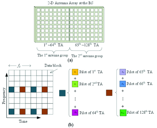
Figure 3: Space-time adaptive pilot scheme, where $M=128$, $N_{G}=2$, $f_{d}=4$, and the adjacent antenna spacing $\lambda/2$ are considered as an example. (a) 2-D antenna array at the BS; (b) Space-time adaptive pilot scheme.

As we have demonstrated in Section II, the spatial common sparsity of MIMO channels is due to the co-located antenna array at the BS. However, for massive MIMO with large antenna array, such common sparsity may not be ensured for antennas spaced apart. To address this problem, we propose that $M$ transmit antennas are divided into $N_{G}$ antenna groups, where $M_{G}=M/N_{G}$ antennas with close distance in the spatial domain are assigned to the same antenna group, so that the spatial common sparsity of wireless MIMO channels in each antenna group can be guaranteed. For example, we consider the $M=128$ planar antenna array as shown in Fig. 3 (a), which can be divided into two array groups according to the criterion above. If we consider $f_{c}=2~{}\rm{GHz}$, $f_{s}=10~{}\rm{MHz}$, and the maximum distance for a pair of antennas in each antenna group as shown in Fig. 3 (a) is $4\sqrt{2}\lambda$, their maximum difference of path delays from the common scatterer is $\frac{{{4\sqrt{2}\lambda}}}{{{c}}}=4\sqrt{2}/f_{c}=0.0028~{}\mu s$, which is negligible compared with the system sample period $T_{s}=1/f_{s}=0.1~{}\mu s$. For a certain antenna group, pilots of different transmit antennas are non-orthogonal and occupy the identical subcarriers, while pilots of different antenna groups are orthogonal in the time domain or frequency domain, which can be illustrated in Fig. 3 (b). For the specific parameter $N_{G}$, we should consider the geometry and scale of the antenna array at the BS, $f_{c}$, and $f_{s}$.

On the other hand, wireless MIMO channels exhibit the temporal correlation. Such temporal channel correlation indicates that during the coherence time of path gains, channels in several successive OFDM symbols can be considered to be quasi-static, and the channel estimation in one OFDM symbol can be used to estimate channels of several adjacent OFDM symbols. This motivates us to further reduce the pilot overhead and increase the available spectrum and energy resources for effective data transmission. To be specific, as illustrated in Fig. 3, every $f_{d}$ adjacent OFDM symbols share the common pilots, where $f_{d}$ is determined by the coherence time of path gains or the mobility of served users.

By exploiting such temporal channel correlation, we can use large $f_{d}$ to reduce the pilot overhead. To estimate channels of OFDM symbols without pilots, we can use interpolation algorithms according to the estimated channels of adjacent OFDM symbols with pilots, e.g., we can adopt the linear interpolation algorithm as follows

$${\hat{\bf{h}}}_{m,r}=[(f_{p}+1-r){{\hat{\bf{h}}}}_{m,1}+(r-1){{\hat{\bf{h}}}}_{m,f_{p}+1}]/f_{p},$$ (11)

where $1<r\leq f_{p}$, ${{\hat{\bf{h}}}}_{m,1}$ and ${{\hat{\bf{h}}}}_{m,f_{p}+1}$ are the estimated channels of the first and ($f_{p}+1$)th OFDM symbols, respectively, and ${\hat{\bf{h}}}_{m,r}$ is the interpolated channel estimation of the $r$th OFDM symbol.

The proposed space-time adaptive pilot scheme considers both the geometry of the antenna array at the BS and the mobility of served users, which can achieve the reliable channel estimation and further reduce the required pilot overhead. For the space-time adaptive pilot scheme, the proposed ASSP algorithm is used at the user to estimate channels associated with different transmit antennas in each antenna group, where the received pilots associated with different antenna groups are processed separately. In Section V, the simulation results will show that the proposed space-time adaptive pilot scheme can further reduce the required pilot overhead with a negligible performance loss, even for the high speed scenario where the users’ mobile velocity is 60 km/h.

III-D Channel Estimation in Multi-Cell Massive MIMO

In this subsection, we extend the proposed channel estimation scheme from the single-cell scenario to the multi-cell scenario. We consider a cellular network composed of ${\cal{L}}=7$ hexagonal cells, each consisting of a central $M$-antenna BS and $K$ single-antenna users that share the same bandwidth, where the users of the central target cell suffer from the interference of the surrounding ${\cal{L}}-1$ interfering cells. One straightforward solution to solve the pilot contamination from the interfering cells is the frequency-division multiplexing (FDM) scheme, i.e., pilots of adjacent cells are orthogonal in the frequency domain. FDM scheme can perfectly mitigate the pilot contamination if the training time used for channel estimation is less than the channel coherence time, but it can lead to the ${\cal{L}}$ times pilot overhead in multi-cell system than that in single-cell system. An alternative solution is the time-division multiplexing (TDM) scheme [36], where pilots of adjacent cells are transmitted in different time slots. The pilot overhead with TDM scheme in multi-cell scenario is the same with that in single-cell scenario. However, the downlink precoded data from adjacent cells may degrade the channel estimation performance of users in the target cell. In Section V, we will verify that the TDM scheme can be the viable approach to mitigate the pilot contamination in multi-cell FDD massive MIMO systems due to the obviously reduced pilot overhead and the slightly performance loss compared to the FDM scheme.

IV Performance Analysis

In this section, we first provide the design of the proposed non-orthogonal pilot scheme for reliable channel estimation under the framework of CS theory. Then we analyze the convergence analysis and complexity of the proposed ASSP algorithm.

IV-A Non-Orthogonal Pilot Design Under the Framework of CS Theory

In CS theory, design of the sensing matrix ${\bf{\Psi}}$ in (9) is very important to effectively and reliably compress the high-dimensional sparse signal $\bf{D}$. For the problem of channel estimation, the design of ${\bf{\Psi}}$ is converted to the design of the pilot placement $\xi$ and the pilot sequences $\left\{{{{\bf{p}}_{m}}}\right\}_{m=1}^{M}$, since the sensing matrix ${\bf{\Psi}}$ is only determined by the parameters $\xi$ and $\left\{{{{\bf{p}}_{m}}}\right\}_{m=1}^{M}$. According to CS theory, the small column correlation of ${\bf{\Psi}}$ is desired for the reliable sparse signal recovery [33], which enlightens us to appropriately design $\xi$ and $\left\{{{{\bf{p}}_{m}}}\right\}_{m=1}^{M}$.

For the specific pilot design, we commence by considering the design of $\left\{{{{\bf{p}}_{m}}}\right\}_{m=1}^{M}$ to achieve the small cross-correlation for columns of ${{\bf{\Psi}}_{l}}$ given any $l$, since this kind of cross-correlation is only determined by $\left\{{{{\bf{p}}_{m}}}\right\}_{m=1}^{M}$, i.e.,

$$\begin{array}[]{l}\!\!\!\!\!\!\!\!({\bm{\psi}}_{{m_{1}},l})^{\rm{H}}{{\bm{\psi}}_{{m_{2}},l}}=({\bf{\Psi}}_{{l}}^{(m_{1})})^{\rm{H}}{\bf{\Psi}}_{{l}}^{(m_{2})}=({\bf{\Phi}}_{{m_{1}}}^{(l)})^{\rm{H}}{\bf{\Phi}}_{{m_{2}}}^{(l)}\\ \!\!\!\!\!\!\!\!{\kern 59.0pt}={({{\bf{p}}_{{m_{1}}}}\circ{\bf{F}}_{p}^{(l)})^{\rm{H}}}({{\bf{p}}_{{m_{2}}}}\circ{\bf{F}}_{p}^{(l)})=({\bf{p}}_{{m_{1}}})^{\rm{H}}{{\bf{p}}_{{m_{2}}}}.\end{array}$$ (12)

where ${\bf{F}}_{p}={\left.{{{\bf{F}}_{L}}}\right|_{\xi}}$ and $1\leq m_{1}<m_{2}\leq M$.

To achieve the small $\left|({{\bm{\psi}}_{{m_{1}},l})^{\rm{H}}{{\bm{\psi}}_{{m_{2}},l}}}\right|$, we consider $\left\{{{\theta_{\kappa,m}}}\right\}_{\kappa=1,m=1}^{{N_{p}},M}$ to follow the independent and identically distributed (i.i.d.) uniform distribution ${\cal{U}}\left[{0,2\pi}\right)$, where ${e^{j{\theta}_{\kappa,m}}}$ denotes the $\kappa$th element of ${{{\bf{p}}_{m}}}\in\mathbb{C}^{{N_{p}}\times 1}$. For the proposed pilot sequences, the $l_{2}$-norm of each column of ${\bf{\Psi}}$ is a constant, i.e., ${\left\|{{{\bm{\psi}}_{m,l}}}\right\|_{2}}=\sqrt{{N_{p}}}$. Meanwhile, we have

$$\mathop{\lim}\limits_{{N_{p}}\to\infty}\frac{{\left|({{\bm{\psi}}_{{m_{1}},{l}})^{\rm{H}}{{\bm{\psi}}_{{m_{2}},{l}}}}\right|}}{{{{\left\|{{{\bm{\psi}}_{{m_{1}},{l}}}}\right\|}_{2}}{{\left\|{{{\bm{\psi}}_{{m_{2}},{l}}}}\right\|}_{2}}}}=\mathop{\lim}\limits_{{N_{p}}\to\infty}\frac{{({\bf{p}}_{{m_{1}}})^{\rm{H}}{{\bf{p}}_{{m_{2}}}}}}{{{N_{p}}}}=0,$$ (13)

which indicates that for the limited $N_{p}$ in practice, the proposed pilot sequences can achieve the good cross-correlation of columns of ${{\bf{\Psi}}_{l}}$ for any $l$ according to the random matrix theory (RMT).

Given the proposed $\left\{{{{\bf{p}}_{m}}}\right\}_{m=1}^{M}$, we further investigate the cross-correlation of ${\bm{\psi}}_{{m_{1}},{l_{1}}}$ and ${{\bm{\psi}}_{{m_{2}},{l_{2}}}}$ with $l_{1}\neq l_{2}$, which enlightens us to design $\xi$ to achieve the small $\left|({\bm{\psi}}_{{m_{1}},{l_{1}}})^{\rm{H}}{{\bm{\psi}}_{{m_{2}},{l_{2}}}}\right|$. In typical massive MIMO systems (e.g., $M\geq 64$), we usually have $N_{p}>L$, which is due to the two following reasons. First, since the number of pilots for estimating the channel associated with one transmit antenna is at least one, the number of the total pilot overhead $N_{p}$ can be at least $64$. Second, since the maximum channel delay spread is $3\sim 5~{}\mu s$ and the typical system bandwidth is $10$ MHz if we refer to the LTE-Advanced system parameters, we have $L\leq 64$ [12]. Based on the condition of $N_{p}>L$, we propose to adopt the widely used uniformly-spaced pilots with the pilot interval $\left\lfloor{\frac{N}{{{N_{p}}}}}\right\rfloor$ to acquire the small $\left|({\bm{\psi}}_{{m_{1}},{l_{1}}})^{\rm{H}}{{\bm{\psi}}_{{m_{2}},{l_{2}}}}\right|$. Specifically, we consider $\xi$ is selected from the set of $\left\{{1,2,\cdots,N}\right\}$ with the equal interval, and the inner product of ${\bm{\psi}}_{{m_{1}},{l_{1}}}$ and ${{\bm{\psi}}_{{m_{2}},{l_{2}}}}$ can be expressed as

$$\!\!\!\!\!\!\!\!\begin{array}[]{l}({\bm{\psi}}_{{m_{1}},{l_{1}}})^{\rm{H}}{{\bm{\psi}}_{{m_{2}},{l_{2}}}}=({\bf{\Phi}}_{{m_{1}}}^{({l_{1}})})^{\rm{H}}{\bf{\Phi}}_{{m_{2}}}^{({l_{2}})}={({{\bf{p}}_{{m_{1}}}}\circ{\bf{F}}_{p}^{({l_{1}})})^{\rm{H}}}({{\bf{p}}_{{m_{2}}}}\circ{\bf{F}}_{p}^{({l_{2}})})\\ {\kern 74.0pt}=\sum\limits_{\kappa=1}^{{N_{p}}}{\exp{{\left({j\frac{{2\pi}}{N}{l_{1}}I\left(\kappa\right)+j{\theta_{\kappa,m_{1}}}}\right)}^{\rm{H}}}}\\ {\kern 90.0pt}\times{\exp{{\left({j\frac{{2\pi}}{N}{l_{2}}I\left(\kappa\right)+j{\theta_{\kappa,m_{2}}}}\right)}}}\\ {\kern 74.0pt}=\sum\limits_{\kappa=1}^{{N_{p}}}{\exp\left({j\frac{{2\pi}}{N}\tilde{l}I\left(\kappa\right)}+{j\Delta{\theta_{\kappa,m}}}\right)},\end{array}$$ (14)

where $\left\{{I\left(\kappa\right)}\right\}_{\kappa=1}^{{N_{p}}}=\xi$ is the indices set of pilot subcarriers, $1\leq{\tilde{l}}=l_{2}-l_{1}\leq L-1$, and $\Delta{\theta_{\kappa,m}}{\rm{=}}{\theta_{\kappa,{m_{2}}}}{\rm{-}}{\theta_{\kappa,{m_{1}}}}$. Furthermore, since $\left\{{I\left(\kappa\right)}\right\}_{\kappa=1}^{{N_{p}}}$ is selected from the set of $\left\{{1,2,\cdots,N}\right\}$ with the equal interval $\left\lfloor{\frac{N}{{{N_{p}}}}}\right\rfloor$, $I\left(\kappa\right)={I_{0}}+(\kappa-1)\left\lfloor{\frac{N}{{{N_{p}}}}}\right\rfloor$ for $1\leq\kappa\leq N_{p}$, where $I_{0}$ is the subcarrier index of the first pilot with $1\leq{I_{0}}<\left\lfloor{\frac{N}{{{N_{p}}}}}\right\rfloor$. Hence, (14) can be also expressed as

$$\!\!\!\begin{array}[]{l}({\bm{\psi}}_{{m_{1}},{l_{1}}})^{\rm{H}}{{\bm{\psi}}_{{m_{2}},{l_{2}}}}=\\ {\kern 15.0pt}{\sum\limits_{\kappa=1}^{{N_{p}}}{\exp\left({j\frac{{2\pi}}{N}\tilde{l}\left({{I_{0}}+(\kappa-1)\left\lfloor{\frac{N}{{{N_{p}}}}}\right\rfloor}\right)+j\Delta{\theta_{\kappa,m}}}\right)}}.\end{array}$$ (15)

Let $\varepsilon=\frac{N}{{{N_{p}}}}-\left\lfloor{\frac{N}{{{N_{p}}}}}\right\rfloor$ with $\varepsilon\in\left[{0,1}\right)$, we can further obtain

$$\!\!\!\!\!\!\!\begin{array}[]{l}({\bm{\psi}}_{{m_{1}},{l_{1}}})^{\rm{H}}{{\bm{\psi}}_{{m_{2}},{l_{2}}}}={c_{0}}\sum\limits_{\kappa=1}^{{N_{p}}}{\exp\left({j\frac{{2\pi}}{N}\tilde{l}\kappa\left({\frac{N}{{{N_{p}}}}-\varepsilon}\right)+{j\Delta{\theta_{\kappa,m}}}}\right)},\end{array}$$ (16)

where $c_{0}=\exp\left({j\frac{{2\pi}}{N}\tilde{l}\left({{I_{0}}-\left\lfloor{\frac{N}{{{N_{p}}}}}\right\rfloor}\right)}\right)$. To investigate $\left|({\bm{\psi}}_{{m_{1}},{l_{1}}})^{\rm{H}}{{\bm{\psi}}_{{m_{2}},{l_{2}}}}\right|$ with $\l_{1}\neq l_{2}$, we consider the following two cases. For the first case, if $m_{1}=m_{2}$, then $\Delta\theta_{\kappa,m}=0$, and (16) can be simplified as

$$\begin{array}[]{l}({\bm{\psi}}_{{m_{1}},{l_{1}}})^{\rm{H}}{{\bm{\psi}}_{{m_{2}},{l_{2}}}}={c_{0}}\sum\limits_{\kappa=1}^{{N_{p}}}{\exp\left({j\frac{{2\pi}}{{{N_{p}}}}\tilde{l}\kappa\left({1-\eta\varepsilon}\right)}\right)},\end{array}$$ (17)

where $\eta=\frac{{{N_{p}}}}{N}<1$ denotes the pilot occupation ratio. Thus, ${\eta\varepsilon\approx 0}$, and we can obtain

$$\mathop{\lim}\limits_{{N_{p}}\to\infty}\frac{({{\bm{\psi}}_{{m_{1}},{l_{1}}})^{\rm{H}}{{\bm{\psi}}_{{m_{2}},{l_{2}}}}}}{{{N_{p}}}}=\mathop{\lim}\limits_{{N_{p}}\to\infty}\frac{{c_{0}\left({1-{e^{j2\pi\tilde{l}\left({1-\eta\varepsilon}\right)}}}\right)}}{{{N_{p}}\left({1-{e^{j\frac{{2\pi}}{{{N_{p}}}}\tilde{l}\left({1-\eta\varepsilon}\right)}}}\right)}}=0,$$ (18)

where ${e^{j\frac{{2\pi}}{{{N_{p}}}}\tilde{l}\left({1-\eta\varepsilon}\right)}}\approx e^{\left({j\frac{{2\pi}}{{{N_{p}}}}\tilde{l}}\right)}\neq 1$ guarantees the validity of (18) due to $1\leq{\tilde{l}}\leq L-1$ and $L<N_{p}$. For the second case, if $m_{1}\neq m_{2}$, then (16) can be expressed as

$$\begin{array}[]{l}({\bm{\psi}}_{{m_{1}},{l_{1}}})^{\rm{H}}{{\bm{\psi}}_{{m_{2}},{l_{2}}}}=\sum\limits_{\kappa=1}^{{N_{p}}}{\exp\left({j{\tilde{\theta}_{\kappa}}}\right)},\end{array}$$ (19)

where ${\tilde{\theta}_{\kappa}}=\frac{{2\pi}}{N}\tilde{l}I\left(\kappa\right){\rm{+}}\Delta{\theta_{\kappa,m}}$ for $1\leq\kappa\leq N_{p}$ follow the i.i.d. distribution ${\cal{U}}\left[{0,2\pi}\right)$. Similar to (13), we further have

$$\begin{array}[]{l}\mathop{\lim}\limits_{{N_{p}}\to\infty}\frac{({{\bm{\psi}}_{{m_{1}},{l_{1}}})^{\rm{H}}{{\bm{\psi}}_{{m_{2}},{l_{2}}}}}}{{{N_{p}}}}=\mathop{\lim}\limits_{{N_{p}}\to\infty}\frac{{\sum\limits_{\kappa=1}^{{N_{p}}}{\exp\left({j{{\tilde{\theta}}_{\kappa}}}\right)}}}{{{N_{p}}}}=0.\end{array}$$ (20)

According to RMT, the asymptotic orthogonality of (13), (18), and (20) indicates that the proposed $\xi$ and $\left\{{{{\bf{p}}_{m}}}\right\}_{m=1}^{M}$ can achieve the good cross-correlation between any two columns of ${{\bf{\Psi}}}$ with the limited $N_{p}$ in practice. Moreover, compared with the conventional random pilot placement scheme widely used in CS-based channel estimation schemes [23], the proposed uniformly-spaced pilot placement scheme can be more easily implemented in practical systems due to its regular pattern. Moreover, it can also facilitate massive MIMO to be backward compatible with current cellular networks, since the uniformly-spaced pilot placement scheme has been widely used in existing cellular networks [13]. Finally, its reliable sparse signal recovery performance can be verified through simulations in Section V.

IV-B Convergence Analysis of Proposed ASSP Algorithm

For the proposed ASSP algorithm, we first provide the convergence with the correct sparsity level $s=P$. Then we provide the convergence for the case of $s\neq P$, where the proposed stopping criteria are also discussed. It should be pointed out that conventional SP algorithm and model-based SP algorithm analyze the convergence for the recovery of a single sparse vector. By contrast, we provide the convergence for the reconstruction of structured sparse matrix.

The convergence for the case of $s=P$ can be guaranteed due to the following theorem.

Theorem 1.

For ${\bf{Y}}={\bf{\Psi D}}+{\bf{W}}$ and the ASSP algorithm with the sparsity level $s=P$, we have

$$\small{\left\|{{\bf{D}}{\rm{-}}{\bf{\hat{D}}}}\right\|_{F}}\leq{c}_{P}{\left\|{\bf{W}}\right\|_{F}},$$ (21)

$$\small{\left\|{{{\bf{R}}^{k}}}\right\|_{F}}<{{c^{\prime}}_{P}}{\left\|{{{\bf{R}}^{k-1}}}\right\|_{F}}+{{c^{\prime\prime}}_{P}}{\left\|{\bf{W}}\right\|_{F}},$$ (22)

where ${\bf{\hat{D}}}$ is the estimation of $\bf{D}$ with $s=P$, and ${c}_{P}$, ${{c^{\prime}}_{P}}$, and ${{c^{\prime\prime}}_{P}}$ are constants.

Here ${c}_{P}$, ${{c^{\prime}}_{P}}$, and ${{c^{\prime\prime}}_{P}}$ are determined by the structured restricted isometry property (SRIP) constants $\delta_{P}$, $\delta_{2P}$, and $\delta_{3P}$, which will be further detailed in Appendix -A. The proof of Theorem 1 will be provided in Appendix -A.

Moreover, we investigate the convergence of the case with $s\neq P$. We consider ${\bf{D}}={\left.{\bf{D}}\right\rangle_{s}}+\left({{\bf{D}}-{{\left.{\bf{D}}\right\rangle}_{s}}}\right)$, where the matrix ${\left.{\bf{D}}\right\rangle_{s}}$ preserves the largest $s$ sub-matrices $\left\{{{{\bf{D}}_{l}}}\right\}_{l=1}^{L}$ according to their $F$-norms and sets other sub-matrices to $\bf{0}$. In this way, (9) can be further expressed as

$${\bf{Y}}={\bf{\Psi}}{\left.{\bf{D}}\right\rangle_{s}}+{\bf{\Psi}}\left({{\bf{D}}-{{\left.{\bf{D}}\right\rangle}_{s}}}\right)+{\bf{W}}={\bf{\Psi}}{\left.{\bf{D}}\right\rangle_{s}}+{\bf{W^{\prime}}},$$ (23)

where ${\bf{W^{\prime}}}={\bf{\Psi}}\left({{\bf{D}}-{{\left.{\bf{D}}\right\rangle}_{s}}}\right)+{\bf{W}}$. For the case of $s\neq P$, we may not reliably reconstruct the $P$-sparse signal $\bf{D}$ even the $s$-sparse signal ${\bf{\mathord{\buildrel{\lower 3.0pt\hbox{$\scriptscriptstyle\smile$}}\over{D}}}}_{s}$ is estimated. However, with the appropriate SRIP, Theorem 1 indicates that we can acquire partial correct support set from the estimated $s$-sparse matrix, i.e., ${\Omega_{s}}\cap{\Omega_{T}}\neq\phi$, where ${\Omega_{s}}$ is the support set of the estimated $s$-sparse matrix, ${\Omega_{T}}$ is the true support set of ${\bf{D}}$, and $\phi$ denotes the null set. Hence ${\Omega_{s}}\cap{\Omega_{T}}\neq\phi$ can reduce the number of iterations for the convergence with the sparsity level $s+1$, since the first iteration with the sparsity level $s+1$ uses ${\Omega_{s}}$ as the priori information (Step 2.2 in Algorithm 1). It should be pointed out that the proof of Theorem 1 does not rely on the estimated support set with the last sparsity level.

Additionally, by exploiting the practical channel property, the proposed stopping criteria enable ASSP algorithm to achieve good MSE performance, and we will discuss the proposed stopping criteria as follows. The stopping criterion ${\left\|{{{\bf{R}}^{k}}}\right\|_{F}}>{\left\|{\bf{R}}_{s-1}\right\|_{F}}$ is clear as it implies that the residue of the current sparsity level is larger than that of the last sparsity level, and stopping the iteration can help the algorithm to acquire the good MSE performance. On the other hand, the stopping criterion ${\left\|{{{{\bf{\mathord{\buildrel{\lower 3.0pt\hbox{$\scriptscriptstyle\smile$}}\over{D}}}}}_{\tilde{l}}}}\right\|_{F}}\leq\sqrt{M_{G}R}{p_{{\rm{th}}}}$ implies that the $\tilde{l}$th path is dominated by AWGN. That is to say, the channel sparsity level is over estimated, although MSE performance with the current sparsity level is better than that with the last sparsity level. Actually, the improvement of MSE performance is due to “reconstructing” noise.

IV-C Computational Complexity of ASSP Algorithm

In each iteration of the proposed ASSP algorithm, the computational complexity mainly comes from the several operations as follows, where the space-time adaptive pilot scheme with $M_{G}$ transmit antennas in each antenna group is considered. For Step 2.1, the correlation operation has the complexity of ${\cal{O}}(RLM_{G}N_{p})$. For Step 2.2, both the support merger and ${\Pi^{s}}\left({\cdot}\right)$ have the complexity of ${\cal{O}}(L)$ [39, 38], while the norm operation has the complexity of ${\cal{O}}(RLM_{G})$. For Step 2.3, the Moore-Penrose matrix inversion operation has the complexity of ${\cal{O}}(2N_{p}({{M_{G}s}})^{2}+({{M_{G}s}})^{3})$ [40], ${\Pi^{s}}\left({\cdot}\right)$ has the complexity of ${\cal{O}}(L)$, and the norm operation has the complexity of ${\cal{O}}(RLM_{G})$. For Step 2.4, the Moore-Penrose matrix inversion operation has the complexity of ${\cal{O}}(2N_{p}({{M_{G}s}})^{2}+({{M_{G}s}})^{3})$. For Step 2.5, the residue update has the complexity of ${\cal{O}}(RLM_{G}N_{p})$. To quantitatively compare the computational complexity of different operations, we consider the parameters used in Fig. 4 when the performance of the proposed ASSP algorithm approaches that of the oracle LS algorithm. In this case, the ratios of the complexity of the correlation operation, the support merger or ${\Pi^{s}}\left({\cdot}\right)$ operation, the norm operation, and the residue update to that of the Moore-Penrose matrix inversion operation are $2.3\times 10^{-2}$, $1.7\times 10^{-6}$, $5.7\times 10^{-5}$, and $2.3\times 10^{-2}$, respectively. Therefore, the main computational complexity of the ASSP algorithm comes from the Moore-Penrose matrix inversion operation with the complexity of ${\cal{O}}(2N_{p}({{M_{G}s}})^{2}+({{M_{G}s}})^{3})$.

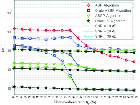
Figure 4: MSE performance comparison of different channel estimation algorithms against pilot overhead ratio and SNR.

V Simulation Results

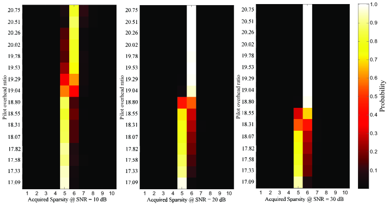
Figure 5: Estimated channel sparsity level of the proposed ASSP algorithm against SNR and pilot overhead ratio.

In this section, a simulation study was carried out to investigate the performance of the proposed channel estimation scheme for FDD massive MIMO systems. To provide a benchmark for performance comparison, we consider the oracle LS algorithm by assuming the true channel support set known at the user and the oracle ASSP algorithm by assuming the true channel sparsity level known at the user. Moreover, to investigate the performance gain from the exploitation of the spatial common sparsity of CIRs, we provide the MSE performance of adaptive subspace pursuit (ASP) algorithm, which is a special case of the proposed ASSP algorithm without leveraging such spatial common sparsity of CIRs. Simulation system parameters were set as: system carrier was $f_{c}=2~{}\rm{GHz}$, system bandwidth was $f_{s}=10~{}\rm{MHz}$, DFT size was $N=4096$, and the length of the guard interval was $N_{g}=64$, which could combat the maximum delay spread of $6.4~{}\mu s$ [12, 41]. We consider the 4 $\times$ 16 planar antenna array ($M=64$), and $M_{G}=32$ is considered to guarantee the spatial common sparsity of channels in each antenna group, the number of pilots to estimate channels for one antenna group is $N_{p}$, and the pilot overhead ratio is $\eta_{p}=(N_{p}M)/(Nf_{p}M_{G})$. The International Telecommunications Union Vehicular-A (ITU-VA) channel model with $P=6$ paths was adopted [12]. Finally, $p_{\rm{th}}$ was set as 0.1, 0.08, 0.06, 0.05, and 0.04 for $\rm{SNR}=10~{}\rm{dB}$, $15~{}\rm{dB}$, $20~{}\rm{dB}$, $25~{}\rm{dB}$, and $30~{}\rm{dB}$, respectively.

Fig. 4 compares the MSE performance of the ASSP algorithm, the oracle ASSP algorithm, the ASP algorithm, and the oracle LS algorithm over static ITU-VA channel. In the simulation, we only consider the channel estimation for one OFDM symbol with $R=1$ and $f_{p}=1$. From Fig. 4, it can be observed that the ASP algorithm performs poorly. The proposed ASSP algorithm outperforms the ASP algorithm, since the spatial common sparsity of MIMO channels is leveraged for the enhanced channel estimation performance. Moreover, for $\eta_{p}\geq 19.04\%$, the ASSP algorithm and the oracle ASSP algorithm have the similar MSE performance, and their performance approaches that of the oracle LS algorithm. This indicates that the proposed ASSP algorithm can reliably acquire the channel sparsity level and the support set for $\eta_{p}\geq 19.04\%$. Moreover, the low pilot overhead implies that the average pilot overhead to estimate the channel associated with one transmit antenna is $N_{p\_{\rm{avg}}}=N_{p}/M_{G}=12.18$, which approaches $2P=12$, the minimum number of observations to reliably recover a $P$-sparse signal [37]. Therefore, the good sparse signal recovery performance of the proposed non-orthogonal pilot scheme and the near-optimal channel estimation performance of the proposed ASSP algorithm are confirmed.

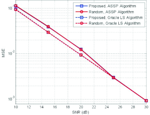
Figure 6: MSE performance comparison of the proposed pilot placement scheme and the conventional random pilot placement scheme.

From Fig. 4, we observe that the ASSP algorithm outperforms the oracle ASSP algorithm for $\eta_{p}<19.04\%$, and its performance is even better than the performance bound obtained by the oracle LS algorithm with $N_{p\_{\rm{avg}}}<2P$ at $\rm{SNR}=10~{}\rm{dB}$. This is because the ASSP algorithm can adaptively acquire the effective channel sparsity level, denoted by $P_{\rm{eff}}$, instead of $P$ can be used to achieve better channel estimation performance. Consider $\eta_{p}=17.09\%$ at $\rm{SNR}=10~{}\rm{dB}$ as an example, we can find that $P_{\rm{eff}}=5$ with high probability for the ASSP algorithm if we refer to Fig. 5. Hence, the average pilot overhead for each transmit antenna $N_{p\_{\rm{avg}}}=N_{p}/M_{G}=10.9$ is still larger than $2P_{\rm{eff}}=10$. From the analysis above, we come to the conclusion that, when $N_{p}$ is insufficient to estimate channels with $P$, the ASSP algorithm will estimate sparse channels with $P_{\rm{eff}}<P$, where path gains accounting for the majority of the channel energy will be estimated, while those with the small energy are discarded as noise. It should be pointed out that the MSE performance fluctuation of the ASSP algorithm at SNR = 10 dB is caused by the fact that $P_{\rm{eff}}$ increases from 5 to 6 when ${\eta_{p}}$ increases, which leads some strong noise to be estimated as the channel paths, and thus degrades the MSE performance.

Fig. 5 depicts the estimated channel sparsity level of the proposed ASSP algorithm against SNR and pilot overhead ratio, where the vertical axis and the horizontal axis represent the used pilot overhead ratio and the adaptively estimated channel sparsity level, respectively, and the chroma denotes the probability of the estimated channel sparsity level. In the simulation, we consider $R=1$ and $f_{p}=1$ without exploiting the temporal channel correlation. Clearly, the proposed ASSP algorithm can acquire the true channel sparsity level with high probability when SNR and pilot overhead ratio increase. Moreover, even in the case of insufficient number of pilots which cannot guarantee the reliable recovery of sparse channels, the proposed ASSP algorithm can still acquire the channel sparsity level with a slight deviation from the true channel sparsity level.

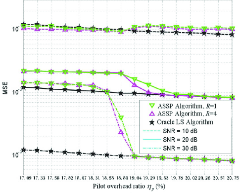
Figure 7: MSE performance comparison of the ASSP algorithm with different $R$’s over time-varying ITU-VA channel with the mobile speed of 60 km/h.

Fig. 6 compares the MSE performance of the proposed pilot placement scheme and the conventional random pilot placement scheme [23], where the proposed ASSP algorithm and the oracle LS algorithm are used. In the simulation, we consider $R=1$, $f_{p}=1$, and ${\eta_{p}}=19.53~{}\%$. Clearly, the proposed pilot placement scheme and the conventional random pilot placement scheme have very similar performance. Due to the regular pilot placement, the proposed uniformly-spaced pilot placement scheme can be more easily implemented in practical systems. Moreover, the uniformly-spaced pilot placement scheme has been used in LTE-Advanced systems, which can facilitate massive MIMO to be backward compatible with current cellular networks [13].

Fig. 7 provides the MSE performance comparison of the proposed ASSP algorithm with ($R=4$) and without ($R=1$) exploiting the temporal common support of wireless channels, where the time-varying ITU-VA channel with the user’s mobile speed of 60 km/h is considered. In the simulation, $f_{p}=1$, and $R=1$ or $4$ denotes the joint processing of the received pilot signals in $R$ successive OFDM symbols. It can be observed that the channel estimation exploiting the temporal channel correlation performs better than that without considering such channel property, especially at low SNR, since more measurements can be used for the improved channel estimation performance. Additionally, by jointly estimating MIMO channels associated with multiple OFDM symbols, we can further reduce the required computational complexity. To be specific, the main computational burden comes from the Moore-Penrose matrix inversion operation as discussed in Section IV-C, and the joint processing of received pilot signals in $R$ OFDM symbols can share the Moore-Penrose matrix inversion operation, which indicates that the complexity can be reduced to $1/R$ of the complexity without using the temporal channel correlation.

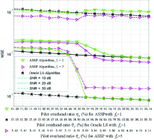
Figure 8: MSE performance comparison of ASSP algorithm with different $f_{d}$’s over time-varying ITU-VA channel with the mobile speed of 60 km/h.

Fig. 8 investigates the performance of the proposed space-time adaptive pilot scheme with different $f_{p}$’s in practical massive MIMO systems, where $R=1$, the time-varying ITU-VA channel with the user’s mobile speed of $60~{}\rm{km/h}$ is considered, and the pilot overhead ratios with different $f_{p}$’s are provided. In the simulation, $f_{d}=1$ and $f_{d}=5$ are considered, and the linear interpolation algorithm is used to estimate channels for OFDM symbols without pilots. From Fig. 8, it can be observed that the case with $f_{d}=5$ only suffers from a negligible performance loss compared to that with $f_{d}=1$ at $\rm{SNR}=30~{}\rm{dB}$. While for $\rm{SNR}\leq 20~{}\rm{dB}$, the case with $f_{d}=5$ is better than that with $f_{d}=1$, since the linear interpolation can reduce the effective noise. By exploiting the temporal channel correlation, the proposed space-time adaptive pilot scheme can substantially reduce the required pilot overhead for channel estimation without the obvious performance loss.

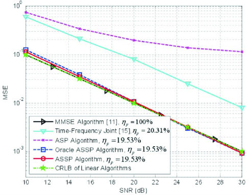
Figure 9: MSE performance comparison of different channel estimation schemes for FDD massive MIMO systems.

Fig. 9 provides the MSE performance comparison of several channel estimation schemes for FDD massive MIMO systems, where we consider the channel estimation for one OFDM symbol with $R=1$ and $f_{p}=1$. The Cramer-Rao lower bound (CRLB) of conventional linear channel estimation schemes (e.g., minimum mean square error (MMSE) algorithm and LS algorithm) is also plotted as the performance benchmark, where ${\mathop{\rm CRLB}}=1/{\rm{SNR}}$ [15]. The ASP algorithm does not perform well due to the insufficient pilots. The time-frequency joint training based scheme [15] works poorly since the mutual interferences of time-domain training sequences of different transmit antennas degrade the channel estimation performance when $M$ is large. Both the MMSE algorithm [10] and the proposed ASSP algorithm achieves 9 dB gain over the scheme proposed in [15], and both of them approach the CRLB of conventional linear algorithms. It is worth mentioning that the proposed scheme enjoys the significantly reduced pilot overhead compared with the MMSE algorithm, since the MMSE algorithm work well only when (8) is well-determined or over-determined. Finally, since the proposed ASSP algorithm can adaptively acquire the channel sparsity level and discards the multipath components buried by the noise at low SNR for improved channel estimation, we can find the proposed scheme even works better than the oracle ASSP algorithm at low SNR.

Fig. 10 and Fig. 11 compare the downlink bit error rate (BER) performance and average achievable throughput per user, respectively, where the BS using zero-forcing (ZF) precoding is assumed to know the estimated downlink channels. In the simulations, the BS with $M=64$ antennas simultaneously serves $K=8$ users using 16-QAM, and the ZF precoding is based on the estimated channels corresponding to Fig. 9 under the same setup. It can be observed that the proposed channel estimation scheme outperforms its counterparts.

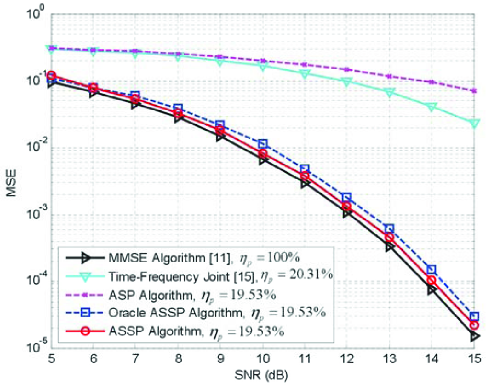
Figure 10: BER performance comparison of different channel estimation schemes for FDD massive MIMO systems.

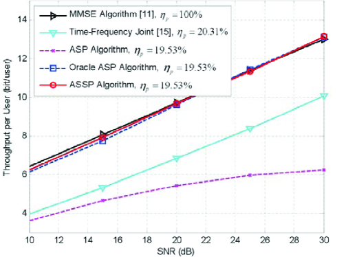
Figure 11: Comparison of average achievable throughput per user of different channel estimation schemes for FDD massive MIMO systems.

Figure 12: Comparison of average achievable throughput per user of different pilot decontamination schemes for multi-cell FDD massive MIMO systems.

Fig. 12 compares the average achievable throughput per user of different pilot decontamination schemes. In the simulations, we consider a multi-cell massive MIMO system with ${\cal{L}}=7$, $M=64$, $K=8$ sharing the same bandwidth, where the average achievable throughput per user in the central target cell suffering from the pilot contamination is investigated. Moreover, we consider $R=1$, $f_{d}=7$, the path loss factor is 3.8 dB/km, the cell radius is 1 km, the distance ${\cal{D}}$ between the BS and its users can be from 100 m to 1 km, the SNR (the power of the unprecoded signal from the BS is considered in SNR) for cell-edge user is 10 dB, the mobile speed of users is 3 km/h. The BSs using zero-forcing (ZF) precoding is assumed to know the estimated downlink channels achieved by the proposed ASSP algorithm. For the FDM scheme, pilots of ${\cal{L}}=7$ cells are orthogonal in the frequency domain. The optimal performance is achieved by the FDM scheme when the users are static. Pilots of ${\cal{L}}=7$ cells in TDM are transmitted in ${\cal{L}}=7$ successive different time slots. In TDM scheme, the channel estimation of users in central target cells suffers from the precoded downlink data transmission of other cells, where two cases are considered. The “cell-edge” case indicates that when users in the central target cell estimate the channels, the precoded downlink data transmission in other cells can guarantee SNR = 10 dB for their cell-edge users. While the “ergodic” case indicates that when users in the central target cell estimate the channels, the precoded downlink data transmission in other cells can guarantee SNR = 10 dB for their users with the the ergodic distance ${\cal{D}}$ from 100 m to 1 km. The negligible performance gap between the FDM scheme and the optimal one is due to the variation of time-varying channels, but it suffers from the high pilot overhead. The TDM scheme with the “cell-edge” case performs worst. While the performance of the TDM scheme with the “ergodic” case approaches that of the optimal one. The simulation results in Fig. 12 indicates that the TDM scheme with low pilot overhead can achieve the good performance when dealing the pilot contamination in multi-cell FDD massive MIMO systems. Moreover, if some appropriate scheduling strategies are considered [36], the performance of the TDM scheme can be further improved.

VI Conclusions

In this paper, we have proposed the SCS-based spatio-temporal joint channel estimation scheme for FDD massive MIMO systems, whereby the intrinsically spatio-temporal common sparsity of wireless MIMO channels is exploited to reduce the pilot overhead. First, the non-orthogonal pilot scheme at the BS and the ASSP algorithm at the user can reliably estimate channels with significantly reduced pilot overhead. Then, the space-time adaptive pilot scheme can further reduce the required pilot overhead according to the mobility of users. Moreover, we discuss the proposed channel estimation scheme in multi-cell scenario. Additionally, we discuss the non-orthogonal pilot design to achieve the reliable channel estimation under the framework of CS theory, and the convergence analysis as well as the complexity analysis of the proposed ASSP algorithm are also provided. Simulation results have shown that the proposed channel estimation scheme can achieve much better channel estimation performance than its counterparts with substantially reduced pilot overhead, and it only suffers from a negligible performance loss when compared with the performance bound.

-A Proof of Theorem 1

We first provide the definition of SRIP for ${\bf{\Psi}}$ in our problem ${\bf{Y}}={\bf{\Psi D}}+{\bf{W}}$ (9), where $\bf{D}$ has the structured sparsity as illustrated in (10). Particularly, the SRIP can be expressed as

$$\small\sqrt{1-\delta}\left\|{\bf{D}}_{\Omega}\right\|_{F}\leq\left\|{{{\bf{\Psi}}_{\Omega}}{\bf{D}}_{\Omega}}\right\|_{F}\leq\sqrt{1+\delta}\left\|{\bf{D}}_{\Omega}\right\|_{F},$$ (24)

where $\delta\in\left[{0,1}\right)$, ${\Omega}$ is an arbitrary set with ${\left|{\Omega}\right|_{c}}\leq P$, and ${\delta_{P}}$ is the infimum of all $\delta$ satisfying (24). Note that for (24), ${\bf{\Psi}}=\left[{{{\bf{\Psi}}_{1}},{{\bf{\Psi}}_{2}},\cdots,{{\bf{\Psi}}_{L}}}\right]\in\mathbb{C}^{{N_{p}}\times ML}$ with ${{\bf{\Psi}}_{l}}\in\mathbb{C}^{{N_{p}}\times M}$ for $1\leq l\leq L$, ${\bf{D}}={\rm{}}{[{\bf{D}}_{1}^{\rm{T}},{\bf{D}}_{2}^{\rm{T}},\cdots,{\bf{D}}_{L}^{\rm{T}}]^{\rm{T}}}\in\mathbb{C}^{ML\times{R}}$ with ${\bf{D}}_{l}\in\mathbb{C}^{M\times{R}}$ for $1\leq l\leq L$, ${{\bf{\Psi}}_{\Omega}}={\left[{{\bf{\Psi}}_{{\Omega(1)}},{\bf{\Psi}}_{{\Omega(2)}},\cdots,{\bf{\Psi}}_{{\Omega({|\Omega|_{c}})}}}\right]}$ and ${{\bf{D}}_{\Omega}}={\left[{{\bf{D}}_{{\Omega(1)}}^{\rm{T}},{\bf{D}}_{{\Omega(2)}}^{\rm{T}},\cdots,{\bf{D}}_{{\Omega({|\Omega|_{c}})}}^{\rm{T}}}\right]^{\rm{T}}}$, and ${\Omega(1)}<{\Omega(2)}<\cdots<{\Omega({|\Omega|_{c}})}$ are elements in the set $\Omega$. Clearly, for two different sparsity levels $P_{1}$ and $P_{2}$ with $P_{1}<P_{2}$, we have $\delta_{P_{1}}\leq\delta_{P_{2}}$. Moreover, for two sets with ${\Omega_{1}}\cap{\Omega_{2}}=\phi$ and the structured sparse matrix $\bf{D}$ with the support set ${\Omega_{2}}$, we have

$$\small{\left\|{{\bf{\Psi}}_{{\Omega_{1}}}^{\rm{H}}{{\bf{\Psi}}}{\bf{D}}}\right\|_{F}}={\left\|{{\bf{\Psi}}_{{\Omega_{1}}}^{\rm{H}}{{\bf{\Psi}}_{{\Omega_{2}}}}{\bf{D}}_{{\Omega_{2}}}}\right\|_{F}}\leq{\delta_{{{\left|{{\Omega_{1}}}\right|}_{c}}+{{\left|{{\Omega_{2}}}\right|}_{c}}}}{\left\|{\bf{D}}\right\|_{F}},$$ (25)

$$\small\begin{array}[]{l}\!\!\!\!(1-\frac{{{\delta_{{{\left|{{\Omega_{1}}}\right|}_{c}}+{{\left|{{\Omega_{2}}}\right|}_{c}}}}}}{{\sqrt{(1-{\delta_{{{\left|{{\Omega_{1}}}\right|}_{c}}}})(1-{\delta_{{{\left|{{\Omega_{2}}}\right|}_{c}}}})}}}){\left\|{{{\bf{\Psi}}_{{\Omega_{2}}}}{{\bf{D}}_{{\Omega_{2}}}}}\right\|_{F}}\\ ~{}~{}~{}~{}~{}~{}~{}~{}\leq{\left\|{({\bf{I}}{\rm{-}}{{\bf{\Psi}}_{{\Omega_{1}}}}{\bf{\Psi}}_{{\Omega_{1}}}^{\dagger}){{\bf{\Psi}}_{{\Omega_{2}}}}{{\bf{D}}_{{\Omega_{2}}}}}\right\|_{F}}\leq{\left\|{{{\bf{\Psi}}_{{\Omega_{2}}}}{{\bf{D}}_{{\Omega_{2}}}}}\right\|_{F}},\end{array}$$ (26)

which will be proven in Appendix -B and -C, respectively.

To prove (21), we need to investigate the upper bound of ${\left\|{{\bf{D}}{\rm{-}}{\bf{\hat{D}}}}\right\|_{F}}$, which can be expressed as

$$\small\begin{array}[]{l}\!\!\!\!\!\!\!\!\!\!{\left\|{{\bf{D}}-{\bf{\hat{D}}}}\right\|_{F}}\leq{\left\|{{{\bf{D}}_{\hat{\Omega}}}-{\bf{\Psi}}_{\hat{\Omega}}^{\dagger}{\bf{Y}}}\right\|_{F}}+{\left\|{{{\bf{D}}_{{\Omega_{T}}/\hat{\Omega}}}}\right\|_{F}}\\ ~{}~{}~{}~{}~{}~{}~{}~{}~{}={\left\|{{{\bf{D}}_{\hat{\Omega}}}-{\bf{\Psi}}_{\hat{\Omega}}^{\dagger}({{\bf{\Psi}}_{{\Omega_{T}}}}{{\bf{D}}_{{\Omega_{T}}}}+{\bf{W}})}\right\|_{F}}+{\left\|{{{\bf{D}}_{{\Omega_{T}}/\hat{\Omega}}}}\right\|_{F}}\\ ~{}~{}~{}~{}~{}~{}~{}~{}~{}\leq{\left\|{{{\bf{D}}_{\hat{\Omega}}}-{\bf{\Psi}}_{\hat{\Omega}}^{\dagger}{{\bf{\Psi}}_{{\Omega_{T}}}}{{\bf{D}}_{{\Omega_{T}}}}}\right\|_{F}}+{\left\|{{\bf{\Psi}}_{\hat{\Omega}}^{\dagger}{\bf{W}}}\right\|_{F}}+{\left\|{{{\bf{D}}_{{\Omega_{T}}/\hat{\Omega}}}}\right\|_{F}}\\ ~{}~{}~{}~{}~{}~{}~{}~{}~{}={\left\|{{\bf{\Psi}}_{\hat{\Omega}}^{\dagger}{{\bf{\Psi}}_{{\Omega_{T}}/\hat{\Omega}}}{{\bf{D}}_{{\Omega_{T}}/\hat{\Omega}}}}\right\|_{F}}+{\left\|{{\bf{\Psi}}_{\hat{\Omega}}^{\dagger}{\bf{W}}}\right\|_{F}}+{\left\|{{{\bf{D}}_{{\Omega_{T}}/\hat{\Omega}}}}\right\|_{F}},\end{array}$$ (27)

where $\hat{\Omega}$ is the estimated support set, $\Omega_{T}$ is the correct support set, and ${{\Omega_{T}}/\hat{\Omega}}$ denotes a set whose elements belong to ${\Omega_{T}}$ except for ${\hat{\Omega}}$. The first inequality is due to $\left\|{\bf{D}}\right\|_{F}^{2}=\left\|{{{\bf{D}}_{\hat{\Omega}}}}\right\|_{F}^{2}+\left\|{{{\bf{D}}_{{\Omega_{T}}/\hat{\Omega}}}}\right\|_{F}^{2}$. The second equality is due to ${{\bf{\Psi}}_{{\Omega_{T}}}}{{\bf{D}}_{{\Omega_{T}}}}={{\bf{\Psi}}_{{\Omega_{T}}/\hat{\Omega}}}{{\bf{D}}_{{\Omega_{T}}/\hat{\Omega}}}+{{\bf{\Psi}}_{{\Omega_{T}}\cap\hat{\Omega}}}{{\bf{D}}_{{\Omega_{T}}\cap\hat{\Omega}}}$ and ${{\bf{D}}_{\hat{\Omega}}}={\bf{\Psi}}_{\hat{\Omega}}^{\dagger}{{\bf{\Psi}}_{{\Omega_{T}}\cap\hat{\Omega}}}{{\bf{D}}_{{\Omega_{T}}\cap\hat{\Omega}}}$.

For ${\left\|{{\bf{\Psi}}_{\hat{\Omega}}^{\dagger}{{\bf{\Psi}}_{{\Omega_{T}}/\hat{\Omega}}}{{\bf{D}}_{{\Omega_{T}}/\hat{\Omega}}}}\right\|_{F}}$, we have

$$\small\begin{array}[]{l}\!\!\!\!\!\!\!\!\!{\left\|{{\bf{\Psi}}_{\hat{\Omega}}^{\dagger}{{\bf{\Psi}}_{{\Omega_{T}}/\hat{\Omega}}}}{{\bf{D}}_{{\Omega_{T}}/\hat{\Omega}}}\right\|_{F}}\\ ={\left\|{{{({\bf{\Psi}}_{\hat{\Omega}}^{\rm{H}}{\bf{\Psi}}_{\hat{\Omega}})}^{-1}}{\bf{\Psi}}_{\hat{\Omega}}^{\rm{H}}{{\bf{\Psi}}_{{\Omega_{T}}/\hat{\Omega}}}}{{\bf{D}}_{{\Omega_{T}}/\hat{\Omega}}}\right\|_{F}}\leq\frac{{{\delta_{2P}}}}{{1-{\delta_{P}}}}{\left\|{{\bf{D}}_{{\Omega_{T}}/\hat{\Omega}}}\right\|_{F}},\end{array}$$ (28)

where the inequality of (28) is due to (24) and (25). Similarly, we have ${\left\|{{\bf{\Psi}}_{\hat{\Omega}}^{\dagger}}{\bf{W}}\right\|_{F}}\leq\frac{{\sqrt{1+{\delta_{P}}}}}{{1-{\delta_{P}}}}{\left\|{\bf{W}}\right\|_{F}}$. Thus we have

$$\small\begin{array}[]{l}\!\!\!\!\!\!\!\!{\left\|{{\bf{D}}-{\bf{\hat{D}}}}\right\|_{F}}\leq\frac{{1-{\delta_{P}}+{\delta_{2P}}}}{{1-{\delta_{P}}}}{\left\|{{{\bf{D}}_{{\Omega_{T}}/\hat{\Omega}}}}\right\|_{F}}+\frac{{\sqrt{1+{\delta_{P}}}}}{{1-{\delta_{P}}}}{\left\|{\bf{W}}\right\|_{F}}.\end{array}$$ (29)

Then we will investigate the relationship between ${\left\|{{{\bf{D}}_{{\Omega_{T}}/\hat{\Omega}}}}\right\|_{F}}$ and ${\left\|{\bf{W}}\right\|_{F}}$. It should be pointed out that, after we get $\hat{\Omega}$, we have ${\left\|{{{\bf{R}}^{k-1}}}\right\|_{F}}\leq{\left\|{\bf{R}}^{k}\right\|_{F}}$, which inspires us to first study the relationship between ${\left\|{{{\bf{R}}^{k}}}\right\|_{F}}$ and ${\left\|{{{\bf{R}}^{k-1}}}\right\|_{F}}$.

For ${\left\|{{{\bf{R}}^{k}}}\right\|_{F}}$, we can obtain

$$\small\begin{array}[]{l}{\left\|{{{\bf{R}}^{k}}}\right\|_{F}}={\left\|{{\bf{\Psi D}}{\rm{+}}{\bf{W}}{\rm{-}}{{\bf{\Psi}}_{{{\tilde{\Omega}}^{k}}}}{\bf{\Psi}}_{{{\tilde{\Omega}}^{k}}}^{\dagger}({\bf{\Psi D}}{\rm{+}}{\bf{W}})}\right\|_{F}}\\ ~{}~{}~{}~{}\leq{\left\|{({\bf{I}}{\rm{-}}{{\bf{\Psi}}_{{{\tilde{\Omega}}^{k}}}}{\bf{\Psi}}_{{{\tilde{\Omega}}^{k}}}^{\dagger}){{\bf{\Psi}}_{{\Omega_{T}}/{{\tilde{\Omega}}^{k}}}}{{\bf{D}}_{{\Omega_{T}}/{{\tilde{\Omega}}^{k}}}}}\right\|_{F}}{\rm{+}}{\left\|{{\bf{W}}{\rm{-}}{{\bf{\Psi}}_{{{\tilde{\Omega}}^{k}}}}{\bf{\Psi}}_{{{\tilde{\Omega}}^{k}}}^{\dagger}{\bf{W}}}\right\|_{F}}\\ ~{}~{}~{}~{}\leq{\left\|{{{\bf{\Psi}}_{{\Omega_{T}}/{{\tilde{\Omega}}^{k}}}}{{\bf{D}}_{{\Omega_{T}}/{{\tilde{\Omega}}^{k}}}}}\right\|_{F}}{\rm{+}}{\left\|{\bf{W}}\right\|_{F}}\\ ~{}~{}~{}~{}\leq\sqrt{1{\rm{+}}{\delta_{P}}}{\left\|{{{\bf{D}}_{{\Omega_{T}}/{{\tilde{\Omega}}^{k}}}}}\right\|_{F}}{\rm{+}}{\left\|{\bf{W}}\right\|_{F}}.\end{array}$$ (30)

where we have ${\bf{\Psi D}}{\rm{=}}{{\bf{\Psi}}_{{\Omega_{T}}\cap{{\tilde{\Omega}}^{k}}}}{{\bf{D}}_{{\Omega_{T}}\cap{{\tilde{\Omega}}^{k}}}}{\rm{+}}{{\bf{\Psi}}_{{\Omega_{T}}/{{\tilde{\Omega}}^{k}}}}{{\bf{D}}_{{\Omega_{T}}/{{\tilde{\Omega}}^{k}}}}$, ${{{\bf{\Psi}}_{{\Omega_{T}}\cap{{\tilde{\Omega}}^{k}}}}{{\bf{D}}_{{\Omega_{T}}\cap{{\tilde{\Omega}}^{k}}}}{\rm{=}}{{\bf{\Psi}}_{{{\tilde{\Omega}}^{k}}}}{\bf{\Psi}}_{{{\tilde{\Omega}}^{k}}}^{\dagger}{{\bf{\Psi}}_{{\Omega_{T}}\cap{{\tilde{\Omega}}^{k}}}}{{\bf{D}}_{{\Omega_{T}}\cap{{\tilde{\Omega}}^{k}}}}}$, and the second inequality is due to (26) and ${\left\|{{\bf{W}}{\rm{-}}{{\bf{\Psi}}_{{{\tilde{\Omega}}^{k}}}}{\bf{\Psi}}_{{{\tilde{\Omega}}^{k}}}^{\dagger}{\bf{W}}}\right\|_{F}}\leq{\left\|{\bf{W}}\right\|_{F}}$.

On the other hand, we consider ${\left\|{{{\bf{R}}^{k-1}}}\right\|_{F}}$, which can be expressed as

$$\small\begin{array}[]{l}\!\!\!{\left\|{{{\bf{R}}^{k{\rm{-}}1}}}\right\|_{F}}\geq{\left\|({\bf{I}}{\rm{-}}{\bf{\Psi}}_{{{\tilde{\Omega}}^{k}}}{{\bf\Psi}}_{{{\tilde{\Omega}}^{k}}}^{\dagger}){{{\bf{\Psi}}_{{\Omega_{T}}/{{\tilde{\Omega}}^{k{\rm{-}}1}}}}{{\bf{D}}_{{\Omega_{T}}/{{\tilde{\Omega}}^{k{\rm{-}}1}}}}}\right\|_{F}}{\rm{-}}{\left\|{\bf{W}}\right\|_{F}}\\ ~{}~{}~{}~{}~{}~{}~{}~{}~{}~{}~{}\geq\frac{{1{\rm{-}}{\delta_{P}}{\rm{-}}{\delta_{2P}}}}{{1{\rm{-}}{\delta_{P}}}}{\left\|{{{\bf{\Psi}}_{{\Omega_{T}}/{{\tilde{\Omega}}^{k{\rm{-}}1}}}}{{\bf{D}}_{{\Omega_{T}}/{{\tilde{\Omega}}^{k{\rm{-}}1}}}}}\right\|_{F}}{\rm{-}}{\left\|{\bf{W}}\right\|_{F}}\\ ~{}~{}~{}~{}~{}~{}~{}~{}~{}~{}~{}\geq\frac{{1{\rm{-}}{\delta_{P}}{\rm{-}}{\delta_{2P}}}}{{\sqrt{1{\rm{-}}{\delta_{P}}}}}{\left\|{{{\bf{D}}_{{\Omega_{T}}/{{\tilde{\Omega}}^{k{\rm{-}}1}}}}}\right\|_{F}}{\rm{-}}{\left\|{\bf{W}}\right\|_{F}},\end{array}$$ (31)

where the second inequality is due to (26).

To further investigate the relationship between (30) and (31), we will derive the relationship between ${\left\|{{{\bf{D}}_{{\Omega_{T}}/{{\tilde{\Omega}}^{k{\rm{}}}}}}}\right\|_{F}}$ and ${\left\|{{{\bf{D}}_{{\Omega_{T}}/{{\tilde{\Omega}}^{k{\rm{-}}1}}}}}\right\|_{F}}$. For convenience, we denote $\Omega_{\Delta}={\Pi^{s}}\left({\left\{{{{\left\|{{{\bf{Z}}_{l}}}\right\|}_{F}}}\right\}_{l=1}^{L}}\right)$ in Step 2.3 of Algorithm 1, then we can get

$$\small\begin{array}[]{l}\!\!\!\!{\left\|{\left.{{\bf{\Psi}}_{{\Omega_{\Delta}}}^{\rm{H}}{\bf{R}}^{k-1}}\right\|}\right._{F}}={\left\|{{\bf{\Psi}}_{{\Omega_{\Delta}}}^{\rm{H}}({\bf{Y}}-{\bf{\Psi}}_{{{\tilde{\Omega}}^{k-1}}}{\bf{\Psi}}_{{{\tilde{\Omega}}^{k-1}}}^{\dagger}{\bf{Y}})}\right\|_{F}}\\ ~{}~{}~{}~{}~{}~{}={\left\|{{\bf{\Psi}}_{{\Omega_{\Delta}}}^{\rm{H}}({\bf{\Psi D}}+{\bf{W}}-{\bf{\Psi}}_{{{\tilde{\Omega}}^{k-1}}}{\bf{\Psi}}_{{{\tilde{\Omega}}^{k-1}}}^{\dagger}({\bf{\Psi D}}+{\bf{W}}))}\right\|_{F}}\\ ~{}~{}~{}~{}~{}~{}\leq{\left.{\left\|{{\bf{\Psi}}_{{\Omega_{\Delta}}}^{\rm{H}}({\bf{\Psi D}}-{\bf{\Psi}}_{{{\tilde{\Omega}}^{k-1}}}{\bf{\Psi}}_{{{\tilde{\Omega}}^{k-1}}}^{\dagger}{\bf{\Psi D}})}\right.}\right\|_{F}}\\ ~{}~{}~{}~{}~{}~{}~{}~{}~{}~{}~{}~{}~{}~{}~{}~{}~{}~{}~{}~{}~{}~{}+{\left.{\left\|{{\bf{\Psi}}_{{\Omega_{\Delta}}}^{\rm{H}}({\bf{W}}-{\bf{\Psi}}_{{{\tilde{\Omega}}^{k-1}}}{\bf{\Psi}}_{{{\tilde{\Omega}}^{k-1}}}^{\dagger}{\bf{W}})}\right.}\right\|_{F}}.\end{array}$$ (32)

For the first part of the right-hand in the inequality of (32), we denote ${\bf{R^{\prime}}}^{k-1}={\bf{\Psi D}}-{\bf{\Psi}}_{{{\tilde{\Omega}}^{k-1}}}{\bf{\Psi}}_{{{\tilde{\Omega}}^{k-1}}}^{\dagger}{\bf{\Psi D}}$, and

$$\small\begin{array}[]{l}\!\!\!{\bf{R^{\prime}}}^{k-1}{\rm{=(}}{\bf{I}}{\rm{-}}{\bf{\Psi}}_{{{\tilde{\Omega}}^{k-1}}}{\bf{\Psi}}_{{{\tilde{\Omega}}^{k-1}}}^{\dagger})({{\bf{\Psi}}_{{\Omega_{T}}/{{\tilde{\Omega}}^{k-1}}}}{{\bf{D}}_{{\Omega_{T}}/{{\tilde{\Omega}}^{k-1}}}}\\ ~{}~{}~{}~{}~{}~{}~{}~{}~{}~{}~{}~{}~{}~{}~{}~{}~{}~{}~{}~{}~{}~{}~{}~{}~{}~{}~{}+{{\bf{\Psi}}_{{\Omega_{T}}\cap{{\tilde{\Omega}}^{k-1}}}}{{\bf{D}}_{{\Omega_{T}}\cap{{\tilde{\Omega}}^{k-1}}}})\\ ~{}~{}~{}~{}~{}~{}=[{{\bf{\Psi}}_{{\Omega_{T}}/{{\tilde{\Omega}}^{k-1}}}},{\bf{\Psi}}_{{{\tilde{\Omega}}^{k-1}}}]\left[{\begin{array}[]{*{20}{c}}{{\bf{D}}_{{\Omega_{T}}/{{\tilde{\Omega}}^{k-1}}}}\\ {-{\bf{\Psi}}_{{{\tilde{\Omega}}^{k-1}}}^{\dagger}{{\bf{\Psi}}_{{\Omega_{T}}/{{\tilde{\Omega}}^{k-1}}}}{{\bf{D}}_{{\Omega_{T}}/{{\tilde{\Omega}}^{k-1}}}}}\end{array}}\right]\\ ~{}~{}~{}~{}~{}~{}={{\bf{\Psi}}_{{\Omega_{T}}\cup{{\tilde{\Omega}}^{k-1}}}}{\bf{\tilde{D}}}^{k-1},\end{array}$$ (33)

where ${\bf{\Psi}}_{{\Omega_{T}}\cup{{\tilde{\Omega}}^{k-1}}}=[{\bf{\Psi}}_{{\Omega_{T}}/{{\tilde{\Omega}}^{k-1}}},{\bf{\Psi}}_{{{\tilde{\Omega}}^{k-1}}}]$ and ${\bf{\tilde{D}}}^{k-1}={[{\bf{D}}_{{\Omega_{T}}/{{\tilde{\Omega}}^{k-1}}}^{\rm{T}},-{({\bf{\Psi}}_{{{\tilde{\Omega}}^{k-1}}}^{\dagger}{{\bf{\Psi}}_{{\Omega_{T}}/{{\tilde{\Omega}}^{k-1}}}}{{\bf{D}}_{{\Omega_{T}}/{{\tilde{\Omega}}^{k-1}}}})^{\rm{T}}}]^{\rm{T}}}$. The second equality of (33) is due to ${{\bf{\Psi}}_{{\Omega_{T}}\cap{{\tilde{\Omega}}^{k-1}}}}{{\bf{D}}_{{\Omega_{T}}\cap{{\tilde{\Omega}}^{k-1}}}}-{\bf{\Psi}}_{{{\tilde{\Omega}}^{k-1}}}{\bf{\Psi}}_{{{\tilde{\Omega}}^{k-1}}}^{\dagger}{{\bf{\Psi}}_{{\Omega_{T}}\cap{{\tilde{\Omega}}^{k-1}}}}{{\bf{D}}_{{\Omega_{T}}\cap{{\tilde{\Omega}}^{k-1}}}}={\bf{0}}$. It should be pointed out that if ${\bf{W}}={\bf{0}}$, we have ${\bf{R^{\prime}}}^{k-1}={\bf{R}}^{k-1}$. For the second part of the right-hand in the inequality of (32), we have

$$\small\begin{array}[]{l}\!\!\!\!\!\!\!\!\!\!{\left.{\left\|{{\bf{\Psi}}_{{\Omega_{\Delta}}}^{\rm{H}}({\bf{W}}-{\bf{\Psi}}_{{{\tilde{\Omega}}^{k-1}}}{\bf{\Psi}}_{{{\tilde{\Omega}}^{k-1}}}^{\dagger}{\bf{W}})}\right.}\right\|_{F}}\\ ~{}={\left.{\left\|{{\bf{\Psi}}_{{\Omega_{\Delta}}}^{\rm{H}}({\bf{I}}-{\bf{\Psi}}_{{{\tilde{\Omega}}^{k-1}}}{\bf{\Psi}}_{{{\tilde{\Omega}}^{k-1}}}^{\dagger}){\bf{W}}}\right.}\right\|_{F}}\leq\sqrt{1+{\delta_{P}}}{\left\|{\bf{W}}\right\|_{F}}.\end{array}$$ (34)

By substituting (33) and (34) into (32), we have

$$\small\begin{array}[]{l}{\left\|{\left.{{\bf{\Psi}}_{{\Omega_{\Delta}}}^{\rm{H}}{\bf{R}}^{k-1}}\right\|}\right._{F}}\leq{\left\|{{\bf{\Psi}}_{{\Omega_{\Delta}}}^{\rm{H}}{{\bf{\Psi}}_{{\Omega_{T}}\cup{{\tilde{\Omega}}^{k-1}}}}{\bf{\tilde{D}}}^{k-1}}\right\|_{F}}+\sqrt{1+{\delta_{P}}}{\left\|{\bf{W}}\right\|_{F}}\\ ~{}~{}~{}~{}~{}~{}~{}~{}~{}~{}~{}~{}~{}~{}~{}~{}~{}~{}~{}={\left\|{{\bf{\Psi}}_{{\Omega_{\Delta}}}^{\rm{H}}}{\bf{R^{\prime}}}^{k-1}\right\|_{F}}+\sqrt{1+{\delta_{P}}}{\left\|{\bf{W}}\right\|_{F}},\end{array}$$ (35)

On the other hand, we have

$$\small\begin{array}[]{l}\!\!\!\!\!\!\!\!\!\!\!\!\!{\left\|{\left.{{\bf{\Psi}}_{{\Omega_{\Delta}}}^{\rm{H}}{\bf{R}}^{k-1}}\right\|}\right._{F}}\mathop{\geq}\limits{\left\|{{\bf{\Psi}}_{{\Omega_{T}}}^{\rm{H}}{\bf{R}}^{k-1}}\right\|_{F}}\\ ~{}~{}~{}~{}~{}~{}~{}~{}~{}~{}~{}~{}\mathop{\geq}\limits{\left.{\left\|{{\bf{\Psi}}_{{\Omega_{T}}}^{\rm{H}}({\bf{\Psi D}}-{\bf{\Psi}}_{{{\tilde{\Omega}}^{k-1}}}{\bf{\Psi}}_{{{\tilde{\Omega}}^{k-1}}}^{\dagger}{\bf{\Psi D}})}\right.}\right\|_{F}}\\ ~{}~{}~{}~{}~{}~{}~{}~{}~{}~{}~{}~{}~{}~{}~{}~{}~{}~{}~{}~{}~{}~{}~{}-{\left.{\left\|{{\bf{\Psi}}_{{\Omega_{T}}}^{\rm{H}}({\bf{W}}-{\bf{\Psi}}_{{{\tilde{\Omega}}^{k-1}}}{\bf{\Psi}}_{{{\tilde{\Omega}}^{k-1}}}^{\dagger}{\bf{W}})}\right.}\right\|_{F}}\\ ~{}~{}~{}~{}~{}~{}~{}~{}~{}~{}~{}~{}\mathop{\geq}\limits{\left.{\left\|{{\bf{\Psi}}_{{\Omega_{T}}}^{\rm{H}}{\bf{R^{\prime}}}^{k-1}}\right.}\right\|_{F}}-\sqrt{1+{\delta_{P}}}{\left\|{\bf{W}}\right\|_{F}}.\end{array}$$ (36)

Combining (35) and (36), we have

$$\small\begin{array}[]{l}\!\!\!\!\!\!\!{\left\|{{\bf{\Psi}}_{{\Omega_{\Delta}}}^{\rm{H}}}{\bf{R^{\prime}}}^{k-1}\right\|_{F}}\geq{\left.{\left\|{{\bf{\Psi}}_{{\Omega_{T}}}^{\rm{H}}{\bf{R^{\prime}}}^{k-1}}\right.}\right\|_{F}}-2\sqrt{1+{\delta_{P}}}{\left\|{\bf{W}}\right\|_{F}}.\end{array}$$ (37)

Due to the following inequality

$$\small{\left\|{{\bf{\Psi}}_{{\Omega_{\Delta}}}^{\rm{H}}}{\bf{R^{\prime}}}^{k-1}\right\|_{F}}\geq{\left\|{{\bf{\Psi}}_{{\Omega_{T}}}^{\rm{H}}{\bf{R}}^{{}^{\prime}k-1}}\right\|_{F}}\geq{\left\|{{\bf{\Psi}}_{{\Omega_{T}}/{\tilde{\Omega}^{k-1}}}^{\rm{H}}{\bf{R}}^{{}^{\prime}k-1}}\right\|_{F}},$$ (38)

(37) can be further expressed as the following inequality by removing the common set of ${\Omega_{\Delta}}$ and ${\Omega_{T}}/{\tilde{\Omega}^{k-1}}$, i.e.,

$$\small\begin{array}[]{l}\!\!\!\!\!\!{\left\|{{\bf{\Psi}}_{{\Omega_{\Delta}}/{\Omega_{T}}}^{\rm{H}}{\bf{R}}^{{}^{\prime}k-1}}\right\|_{F}}\geq{\left\|{{\bf{\Psi}}_{\{{\Omega_{T}}/{\tilde{\Omega}^{k-1}}\}/{\Omega_{\Delta}}}^{\rm{H}}{\bf{R}}^{{}^{\prime}k-1}}\right\|_{F}}-2\sqrt{1+{\delta_{P}}}{\left\|{\bf{W}}\right\|_{F}},\end{array}$$ (39)

here ${\left\|{{\bf{\Psi}}_{\{{\Omega_{T}}/{\tilde{\Omega}^{k-1}}\}/{\Omega_{\Delta}}}^{\rm{H}}{\bf{R}}^{{}^{\prime}k-1}}\right\|_{F}}$ can be expressed as

$$\small\begin{array}[]{l}\!\!\!\!\!\!\!\!\!\!\!\!\!\!{\left\|{{\bf{\Psi}}_{\{{\Omega_{T}}/{\tilde{\Omega}^{k-1}}\}/{\Omega_{\Delta}}}^{\rm{H}}{\bf{R}}^{{}^{\prime}k-1}}\right\|_{F}}={\left\|{{\bf{\Psi}}_{{\Omega_{T}}/{{\tilde{\Omega}}^{{}^{\prime}k}}}^{\rm{H}}{\bf{R}}^{{}^{\prime}k-1}}\right\|_{F}}\\ ={\left\|{{\bf{\Psi}}_{{\Omega_{T}}/{{\tilde{\Omega}}^{{}^{\prime}k}}}^{\rm{H}}{{\bf{\Psi}}_{{\Omega_{T}}\cup{{\tilde{\Omega}}^{k-1}}}}{\bf{\tilde{D}}}^{k-1}}\right\|_{F}}\\ =\left\|{{\bf{\Psi}}_{{\Omega_{T}}/{{\tilde{\Omega}}^{{}^{\prime}k}}}^{\rm{H}}({{\bf{\Psi}}_{\{{\Omega_{T}}\cup{{\tilde{\Omega}}^{k-1}}\}/\{{\Omega_{T}}/{{\tilde{\Omega}}^{{}^{\prime}k}}\}}}{\bf{\tilde{D}}}_{\{{\Omega_{T}}\cup{{\tilde{\Omega}}^{k-1}}\}/\{{\Omega_{T}}/{{\tilde{\Omega}}^{{}^{\prime}k}}\}}^{k-1}}\right.\\ ~{}~{}~{}~{}~{}~{}~{}~{}~{}~{}~{}~{}~{}~{}+{\left.{{{\bf{\Psi}}_{{\Omega_{T}}/{{\tilde{\Omega}}^{{}^{\prime}k}}}}{\bf{\tilde{D}}}_{{\Omega_{T}}/{{\tilde{\Omega}}^{{}^{\prime}k}}}^{k-1})}\right\|_{F}}\\ \geq{\left.{\left\|{{{\bf{\Psi}}^{\rm{H}}_{{\Omega_{T}}/{{\tilde{\Omega}}^{{}^{\prime}k}}}}{{\bf{\Psi}}_{{\Omega_{T}}/{{\tilde{\Omega}}^{{}^{\prime}k}}}}{\bf{\tilde{D}}}_{{\Omega_{T}}/{{\tilde{\Omega}}^{{}^{\prime}k}}}^{k-1}}\right.}\right\|_{F}}\\ ~{}~{}~{}~{}-{\left.{\left\|{{\bf{\Psi}}_{{\Omega_{T}}/{{\tilde{\Omega}}^{{}^{\prime}k}}}^{\rm{H}}{{\bf{\Psi}}_{\{{\Omega_{T}}\cup{{\tilde{\Omega}}^{k-1}}\}/\{{\Omega_{T}}/{{\tilde{\Omega}}^{{}^{\prime}k}}\}}}{\bf{\tilde{D}}}_{\{{\Omega_{T}}\cup{{\tilde{\Omega}}^{k-1}}\}/\{{\Omega_{T}}/{{\tilde{\Omega}}^{{}^{\prime}k}}\}}^{k-1}}\right.}\right\|_{F}}\\ \geq(1-{\delta_{P}}){\left\|{{\bf{\tilde{D}}}_{{\Omega_{T}}/{{\tilde{\Omega}}^{{}^{\prime}k}}}^{k-1}}\right\|_{F}}-{\delta_{3P}}{\left\|{{\bf{\tilde{D}}}^{k-1}}\right\|_{F}}\\ =(1-{\delta_{P}}){\left\|{{\bf{D}}_{{\Omega_{T}}/{{\tilde{\Omega}}^{{}^{\prime}k}}}}\right\|_{F}}-{\delta_{3P}}{\left\|{{\bf{\tilde{D}}}^{k-1}}\right\|_{F}},\end{array}$$ (40)

where the first equality is due to ${\Omega_{\Delta}}\cap{{\tilde{\Omega}}^{k-1}}=\phi$ and ${\Omega_{\Delta}}\cup{\tilde{\Omega}^{k-1}}={\tilde{\Omega}^{\prime k}}$, the second equality is due to (33), and the last equality is due to the definition of ${\bf{\tilde{D}}}^{k-1}$. Since ${\left\|{{\bf{\Psi}}_{{\Omega_{\Delta}}/{\Omega_{T}}}^{\rm{H}}{\bf{R}}^{{}^{\prime}k-1}}\right\|_{F}}={\left\|{{\bf{\Psi}}_{{\Omega_{\Delta}}/{\Omega_{T}}}^{\rm{H}}{{\bf{\Psi}}_{{\Omega_{T}}\cup{{\tilde{\Omega}}^{k-1}}}}{\bf{\tilde{D}}}^{k-1}}\right\|_{F}}\leq{\delta_{3P}}{\left\|{{\bf{\tilde{D}}}^{k-1}}\right\|_{F}}$, by substituting (40) into (39), we have

$$\begin{array}[]{l}(1-{\delta_{P}}){\left\|{{\bf{D}}_{{\Omega_{T}}/{{\tilde{\Omega}}^{{}^{\prime}k}}}}\right\|_{F}}\leq 2{\delta_{3P}}{\left\|{{\bf{\tilde{D}}}^{k-1}}\right\|_{F}}+2\sqrt{1+{\delta_{P}}}{\left\|{\bf{W}}\right\|_{F}}.\end{array}$$ (41)

It should be pointed out that for ${\left\|{{\bf{\tilde{D}}}^{k-1}}\right\|_{F}}$, we can further get

$$\small\begin{array}[]{l}{\left\|{{\bf{\tilde{D}}}^{k-1}}\right\|_{F}}\leq{\left\|{{\bf{D}}_{{\Omega_{T}}/{{\tilde{\Omega}}^{k-1}}}}\right\|_{F}}+{\left\|{{\bf{\Psi}}_{{{\tilde{\Omega}}^{k-1}}}^{\dagger}{{\bf{\Psi}}_{{\Omega_{T}}/{{\tilde{\Omega}}^{k-1}}}}{{\bf{D}}_{{\Omega_{T}}/{{\tilde{\Omega}}^{k-1}}}}}\right\|_{F}}\\ ~{}~{}~{}~{}~{}~{}~{}~{}~{}~{}~{}~{}={\left\|{{\bf{D}}_{{\Omega_{T}}/{{\tilde{\Omega}}^{k-1}}}}\right\|_{F}}\\ ~{}~{}~{}~{}~{}~{}~{}~{}~{}~{}~{}~{}~{}~{}+{\left\|{{{({\bf{\Psi}}_{{{\tilde{\Omega}}^{k-1}}}^{\rm{H}}{\bf{\Psi}}_{{{\tilde{\Omega}}^{k-1}}})}^{-1}}{\bf{\Psi}}_{{{\tilde{\Omega}}^{k-1}}}^{\rm{H}}{{\bf{\Psi}}_{{\Omega_{T}}/{{\tilde{\Omega}}^{k-1}}}}{{\bf{D}}_{{\Omega_{T}}/{{\tilde{\Omega}}^{k-1}}}}}\right\|_{F}}\\ ~{}~{}~{}~{}~{}~{}~{}~{}~{}~{}~{}~{}\leq{\left\|{{\bf{D}}_{{\Omega_{T}}/{{\tilde{\Omega}}^{k-1}}}}\right\|_{F}}+\frac{{{\delta_{2P}}}}{{1-{\delta_{P}}}}{\left\|{{{\bf{D}}_{{\Omega_{T}}/{{\tilde{\Omega}}^{k-1}}}}}\right\|_{F}}\\ ~{}~{}~{}~{}~{}~{}~{}~{}~{}~{}~{}~{}=\frac{1-{\delta_{P}}+{\delta_{2P}}}{{1-{\delta_{P}}}}{\left\|{{{\bf{D}}_{{\Omega_{T}}/{{\tilde{\Omega}}^{k-1}}}}}\right\|_{F}},\end{array}$$ (42)

where the first inequality is due to the definition of ${\bf{\tilde{D}}}^{k-1}$. By substituting (41) into (42), we have

$$\small\begin{array}[]{l}{\left\|{{{\bf{D}}_{{\Omega_{T}}/{{\tilde{\Omega}}^{k-1}}}}}\right\|_{F}}\geq\frac{{{{(1-{\delta_{P}})}^{2}}}}{{2{\delta_{3P}}(1{\rm{-}}{\delta_{P}}{\rm{+}}{\delta_{2P}})}}{\left\|{{{\bf{D}}_{{\Omega_{T}}/{{\tilde{\Omega}}^{{}^{\prime}k}}}}}\right\|_{F}}\\ ~{}~{}~{}~{}~{}~{}~{}~{}~{}~{}~{}~{}~{}~{}~{}~{}~{}~{}~{}~{}~{}~{}~{}-\frac{{\sqrt{1+{\delta_{P}}}(1{\rm{-}}{\delta_{P}})}}{{{\delta_{3P}}(1{\rm{-}}{\delta_{P}}{\rm{+}}{\delta_{2P}})}}{\left\|{\bf{W}}\right\|_{F}}.\end{array}$$ (43)

Then, we investigate ${{{\bf{D}}_{{\Omega_{T}}/{{\tilde{\Omega}}^{k}}}}}$, which can be expressed as

$$\small\begin{array}[]{l}{\left\|{{{\bf{D}}_{{\Omega_{T}}/{{\tilde{\Omega}}^{k}}}}}\right\|_{F}}={\left\|{{{\bf{D}}_{{\Omega_{T}}\cap\{{{\tilde{\Omega}}^{{}^{\prime}k}}/{{\tilde{\Omega}}^{k}}\}+{\Omega_{T}}/{{\tilde{\Omega}}^{{}^{\prime}k}}}}}\right\|_{F}}\\ ~{}~{}~{}~{}~{}~{}~{}~{}~{}~{}~{}~{}~{}~{}~{}\leq{\left\|{{{\bf{D}}_{{\Omega_{T}}\cap\{{{\tilde{\Omega}}^{{}^{\prime}k}}/{{\tilde{\Omega}}^{k}}\}}}}\right\|_{F}}+{\left\|{{{\bf{D}}_{{\Omega_{T}}/{{\tilde{\Omega}}^{{}^{\prime}k}}}}}\right\|_{F}}\\ ~{}~{}~{}~{}~{}~{}~{}~{}~{}~{}~{}~{}~{}~{}~{}={\left\|{{{\bf{D}}_{{{\tilde{\Omega}}^{{}^{\prime}k}}/{{\tilde{\Omega}}^{k}}}}}\right\|_{F}}+{\left\|{{{\bf{D}}_{{\Omega_{T}}/{{\tilde{\Omega}}^{{}^{\prime}k}}}}}\right\|_{F}},\end{array}$$ (44)

where we use the fact that ${{\tilde{\Omega}}^{k}}\subset{{\tilde{\Omega}}^{{}^{\prime}k}}$. For ${\left\|{{{\bf{D}}_{{{\tilde{\Omega}}^{{}^{\prime}k}}/{{\tilde{\Omega}}^{k}}}}}\right\|_{F}}$, we can further obtain

$$\small\begin{array}[]{l}{\left\|{{{\bf{D}}_{{{\tilde{\Omega}}^{{}^{\prime}k}}/{{\tilde{\Omega}}^{k}}}}}\right\|_{F}}={\left\|{{{{{{\bf{\mathord{\buildrel{\lower 3.0pt\hbox{$\scriptscriptstyle\smile$}}\over{D}}}}}_{{{\tilde{\Omega}}^{{}^{\prime}k}}\cap\{{{{\tilde{\Omega}}^{{}^{\prime}k}}/{{\tilde{\Omega}}^{k}}}\}}}+{\bf{E}}}_{{{\tilde{\Omega}}^{{}^{\prime}k}}/{{\tilde{\Omega}}^{k}}}}}\right\|_{F}}\\ ~{}~{}~{}~{}~{}~{}~{}~{}~{}~{}~{}~{}~{}~{}~{}~{}\leq{\left\|{{{\bf{\mathord{\buildrel{\lower 3.0pt\hbox{$\scriptscriptstyle\smile$}}\over{D}}}}}_{{{\tilde{\Omega}}^{{}^{\prime}k}}\cap\{{{{\tilde{\Omega}}^{{}^{\prime}k}}/{{\tilde{\Omega}}^{k}}}\}}}\right\|_{F}}+{\left\|{{{\bf{E}}_{{{\tilde{\Omega}}^{{}^{\prime}k}}/{{\tilde{\Omega}}^{k}}}}}\right\|_{F}}\\ ~{}~{}~{}~{}~{}~{}~{}~{}~{}~{}~{}~{}~{}~{}~{}~{}\leq{\left\|{{{\bf{\mathord{\buildrel{\lower 3.0pt\hbox{$\scriptscriptstyle\smile$}}\over{D}}}}}_{{{\tilde{\Omega}}^{{}^{\prime}k}}\cap{\Omega^{\prime}}}}\right\|_{F}}+{\left\|{{{\bf{E}}_{{{\tilde{\Omega}}^{{}^{\prime}k}}/{{\tilde{\Omega}}^{k}}}}}\right\|_{F}}\\ ~{}~{}~{}~{}~{}~{}~{}~{}~{}~{}~{}~{}~{}~{}~{}~{}={\left\|{{{{\bf{D}}_{{{\tilde{\Omega}}^{{}^{\prime}k}}\cap{\Omega^{\prime}}}-{\bf{E}}}_{\Omega^{\prime}}}}\right\|_{F}}+{\left\|{{{\bf{E}}_{{{\tilde{\Omega}}^{{}^{\prime}k}}/{{\tilde{\Omega}}^{k}}}}}\right\|_{F}}\\ ~{}~{}~{}~{}~{}~{}~{}~{}~{}~{}~{}~{}~{}~{}~{}~{}\leq{\left\|{{{\bf{D}}_{\Omega^{\prime}}}}\right\|_{F}}+{\left\|{{{\bf{E}}_{\Omega^{\prime}}}}\right\|_{F}}+{\left\|{{{\bf{E}}_{{{\tilde{\Omega}}^{{}^{\prime}k}}/{{\tilde{\Omega}}^{k}}}}}\right\|_{F}}\\ ~{}~{}~{}~{}~{}~{}~{}~{}~{}~{}~{}~{}~{}~{}~{}~{}={\bf{0}}+{\left\|{{{\bf{E}}_{\Omega^{\prime}}}}\right\|_{F}}+{\left\|{{{\bf{E}}_{{{\tilde{\Omega}}^{{}^{\prime}k}}/{{\tilde{\Omega}}^{k}}}}}\right\|_{F}}\\ ~{}~{}~{}~{}~{}~{}~{}~{}~{}~{}~{}~{}~{}~{}~{}~{}\leq 2{\left\|{\bf{E}}\right\|_{F}},\end{array}$$ (45)

where we introduce the error variable ${\bf{E}}={\bf{D}}_{{{\tilde{\Omega}}^{{}^{\prime}k}}}-{{{\bf{\mathord{\buildrel{\lower 3.0pt\hbox{$\scriptscriptstyle\smile$}}\over{D}}}}}_{{{\tilde{\Omega}}^{{}^{\prime}k}}}}$ (${{{\bf{\mathord{\buildrel{\lower 3.0pt\hbox{$\scriptscriptstyle\smile$}}\over{D}}}}}_{{{\tilde{\Omega}}^{{}^{\prime}k}}}}$ is obtained in Step 2.3 of Algorithm 1), and $\Omega^{\prime}$ is an arbitrary set satisfying ${\left|{\Omega^{\prime}}\right|_{c}}=P$, $\Omega^{\prime}\subset{{\tilde{\Omega}}^{{}^{\prime}k}}$, and $\Omega^{\prime}\cap{\Omega_{T}}=\phi$. The second inequality in (45) is due to the fact that ${{{\tilde{\Omega}}^{{}^{\prime}k}}/{{\tilde{\Omega}}^{k}}}$ is the discarded support in the step of support pruning in Algorithm 1. According to the definition of ${\bf{E}}$, we further obtain

$$\small\begin{array}[]{l}{\left\|{\bf{E}}\right\|_{F}}={\left\|{{{\bf{D}}_{{{\tilde{\Omega}}^{{}^{\prime}k}}}}-{{{\bf{\mathord{\buildrel{\lower 3.0pt\hbox{$\scriptscriptstyle\smile$}}\over{D}}}}}_{{{\tilde{\Omega}}^{{}^{\prime}k}}}}}\right\|_{F}}{\rm{=}}{\left\|{{{\bf{D}}_{{{\tilde{\Omega}}^{{}^{\prime}k}}}}-{\bf{\Psi}}_{{{\tilde{\Omega}}^{{}^{\prime}k}}}^{\dagger}{\bf{Y}}}\right\|_{F}}\\ ~{}~{}~{}~{}~{}~{}~{}~{}{\rm{=}}{\left\|{{{\bf{D}}_{{{\tilde{\Omega}}^{{}^{\prime}k}}}}-{\bf{\Psi}}_{{{\tilde{\Omega}}^{{}^{\prime}k}}}^{\dagger}({\bf{\Psi D}}+{\bf{W}})}\right\|_{F}}\\ ~{}~{}~{}~{}~{}~{}~{}\leq{\left\|{{{\bf{D}}_{{{\tilde{\Omega}}^{{}^{\prime}k}}}}-{\bf{\Psi}}_{{{\tilde{\Omega}}^{{}^{\prime}k}}}^{\dagger}{\bf{\Psi D}}}\right\|_{F}}{\rm{+}}{\left\|{{\bf{\Psi}}_{{{\tilde{\Omega}}^{{}^{\prime}k}}}^{\dagger}{\bf{W}}}\right\|_{F}}\\ ~{}~{}~{}~{}~{}~{}~{}={\left\|{{{\bf{D}}_{{{\tilde{\Omega}}^{{}^{\prime}k}}}}-{\bf{\Psi}}_{{{\tilde{\Omega}}^{{}^{\prime}k}}}^{\dagger}{\bf{\Psi}}_{\Omega_{T}}{{\bf D}}_{\Omega_{T}}}\right\|_{F}}{\rm{+}}{\left\|{{\bf{\Psi}}_{{{\tilde{\Omega}}^{{}^{\prime}k}}}^{\dagger}{\bf{W}}}\right\|_{F}}.\end{array}$$ (46)

For ${\left\|{{{\bf{D}}_{{{\tilde{\Omega}}^{{}^{\prime}k}}}}-{\bf{\Psi}}_{{{\tilde{\Omega}}^{{}^{\prime}k}}}^{\dagger}{{\bf{\Psi}}_{{\Omega_{T}}}}{{\bf{D}}_{{\Omega_{T}}}}}\right\|_{F}}$, we can have

$$\small\begin{array}[]{l}{\left\|{{{\bf{D}}_{{{\tilde{\Omega}}^{{}^{\prime}k}}}}-{\bf{\Psi}}_{{{\tilde{\Omega}}^{{}^{\prime}k}}}^{\dagger}{{\bf{\Psi}}_{{\Omega_{T}}}}{{\bf{D}}_{{\Omega_{T}}}}}\right\|_{F}}\\ ={\left\|{{{\bf{D}}_{{{\tilde{\Omega}}^{{}^{\prime}k}}}}-{\bf{\Psi}}_{{{\tilde{\Omega}}^{{}^{\prime}k}}}^{\dagger}({{\bf{\Psi}}_{{\Omega_{T}}\cap{{\tilde{\Omega}}^{{}^{\prime}k}}}}{{\bf{D}}_{{\Omega_{T}}\cap{{\tilde{\Omega}}^{{}^{\prime}k}}}}+{{\bf{\Psi}}_{{\Omega_{T}}/{{\tilde{\Omega}}^{{}^{\prime}k}}}}{{\bf{D}}_{{\Omega_{T}}/{{\tilde{\Omega}}^{{}^{\prime}k}}}})}\right\|_{F}}\\ ={\left\|{({{\bf{D}}_{{{\tilde{\Omega}}^{{}^{\prime}k}}}}\!\!-\!\!{\bf{\Psi}}_{{{\tilde{\Omega}}^{{}^{\prime}k}}}^{\dagger}{{\bf{\Psi}}_{{\Omega_{T}}\cap{{\tilde{\Omega}}^{{}^{\prime}k}}}}{{\bf{D}}_{{\Omega_{T}}\cap{{\tilde{\Omega}}^{{}^{\prime}k}}}})\!\!-\!\!{\bf{\Psi}}_{{{\tilde{\Omega}}^{{}^{\prime}k}}}^{\dagger}{{\bf{\Psi}}_{{\Omega_{T}}/{{\tilde{\Omega}}^{{}^{\prime}k}}}}{{\bf{D}}_{{\Omega_{T}}/{{\tilde{\Omega}}^{{}^{\prime}k}}}}}\!\right\|_{F}}\\ ={\left\|{({{\bf{D}}_{{{\tilde{\Omega}}^{{}^{\prime}k}}}}-{\bf{\Psi}}_{{{\tilde{\Omega}}^{{}^{\prime}k}}}^{\dagger}{{\bf{\Psi}}_{{{\tilde{\Omega}}^{{}^{\prime}k}}}}{{\bf{D}}_{{{\tilde{\Omega}}^{{}^{\prime}k}}}})-{\bf{\Psi}}_{{{\tilde{\Omega}}^{{}^{\prime}k}}}^{\dagger}{{\bf{\Psi}}_{{\Omega_{T}}/{{\tilde{\Omega}}^{{}^{\prime}k}}}}{{\bf{D}}_{{\Omega_{T}}/{{\tilde{\Omega}}^{{}^{\prime}k}}}}}\right\|_{F}}\\ ={\left\|{{{\bf{D}}_{{{\tilde{\Omega}}^{{}^{\prime}k}}}}-{{\bf{D}}_{{{\tilde{\Omega}}^{{}^{\prime}k}}}}-{\bf{\Psi}}_{{{\tilde{\Omega}}^{{}^{\prime}k}}}^{\dagger}{{\bf{\Psi}}_{{\Omega_{T}}/{{\tilde{\Omega}}^{{}^{\prime}k}}}}{{\bf{D}}_{{\Omega_{T}}/{{\tilde{\Omega}}^{{}^{\prime}k}}}}}\right\|_{F}}\\ ={\left\|{{\bf{\Psi}}_{{{\tilde{\Omega}}^{{}^{\prime}k}}}^{\dagger}{{\bf{\Psi}}_{{\Omega_{T}}/{{\tilde{\Omega}}^{{}^{\prime}k}}}}{{\bf{D}}_{{\Omega_{T}}/{{\tilde{\Omega}}^{{}^{\prime}k}}}}}\right\|_{F}}\\ \leq\frac{{{\delta_{3P}}}}{{1{\rm{-}}{\delta_{2P}}}}{\left\|{{{\bf{D}}_{{\Omega_{T}}/{{\tilde{\Omega}}^{{}^{\prime}k}}}}}\right\|_{F}},\end{array}$$ (47)

where the last inequality is due to $|{{\tilde{\Omega}}^{{}^{\prime}k}}|_{c}=2P$. While for ${\left\|{{\bf{\Psi}}_{{{\tilde{\Omega}}^{{}^{\prime}k}}}^{\dagger}{\bf{W}}}\right\|_{F}}$ in (46), we have

$$\small{\left\|{{\bf{\Psi}}_{{{\tilde{\Omega}}^{{}^{\prime}k}}}^{\dagger}{\bf{W}}}\right\|_{F}}\leq{\delta_{2P}}/\sqrt{1{\rm{-}}{\delta_{2P}}}{\left\|{\bf{W}}\right\|_{F}}.$$ (48)

By substituting (45)-(48) into (44), we can obtain

$$\small{\left\|{{{\bf{D}}_{{\Omega_{T}}/{{\tilde{\Omega}}^{{}^{\prime}k}}}}}\right\|_{F}}\geq\frac{{(1{\rm{-}}{\delta_{2P}}){{\left\|{{{\bf{D}}_{{\Omega_{T}}/{{\tilde{\Omega}}^{k}}}}}\right\|}_{F}}-2{\delta_{P}}\sqrt{1{\rm{-}}{\delta_{2P}}}{{\left\|{\bf{W}}\right\|}_{F}}}}{{1{\rm{-}}{\delta_{2P}}+2{\delta_{3P}}}}.$$ (49)

Furthermore, by substituting (49) into (43), we can obtain

$$\small\begin{array}[]{*{20}{l}}\!\!\!\!\!{{{\left\|{{{\bf{D}}_{{\Omega_{T}}/{{\tilde{\Omega}}^{k-1}}}}}\right\|}_{F}}\geq\underbrace{\frac{{{{(1-{\delta_{P}})}^{2}}(1-{\delta_{2P}})}}{{2{\delta_{3P}}(1-{\delta_{P}}+{\delta_{2P}})(1-{\delta_{2P}}+{\delta_{3P}})}}}_{{C_{1}}}{{\left\|{{{\bf{D}}_{{\Omega_{T}}/{{\tilde{\Omega}}^{k}}}}}\right\|}_{F}}}\\ \!\!\!\!\!-\underbrace{\frac{{(1-{\delta_{P}})}}{{{\delta_{3P}}(1-{\delta_{P}}+{\delta_{2P}})}}(\frac{{{\delta_{P}}(1-{\delta_{P}})\sqrt{1-{\delta_{2P}}}}}{{(1-{\delta_{2P}}+2{\delta_{3P}})}}+\sqrt{1+{\delta_{P}}})}_{{C_{2}}}{\left\|{\bf{W}}\right\|_{F}}.\end{array}$$ (50)

As we have discussed, if ${\left\|{{{\bf{R}}^{k-1}}}\right\|_{F}}\leq{\left\|{\bf{R}}^{k}\right\|_{F}}$, the iteration quits, which indicates that the estimation of the $P$-sparse signal $\bf{D}$ is obtained, and $\hat{\Omega}={{\tilde{\Omega}}^{k-1}}$. Then we can combine (30), (31), and (50) to obtain

$$\small{\left\|{{{\bf{D}}_{{\Omega_{T}}/\hat{\Omega}}}}\right\|_{F}}\leq C_{3}{\left\|{\bf{W}}\right\|_{F}},$$ (51)

where ${C_{3}}=\frac{{2{C_{1}}\sqrt{1-\delta_{P}}+{C_{2}}\sqrt{1-\delta_{P}^{2}}}}{{{C_{1}}(1-{\delta_{P}}-{\delta_{2P}})-\sqrt{1-\delta_{P}^{2}}}}$. By substituting (29) into (51), we have

$$\small{\left\|{{\bf{D}}-{\bf{\hat{D}}}}\right\|_{F}}\leq C_{4}{\left\|{\bf{W}}\right\|_{F}},$$ (52)

where ${C_{4}}=\frac{{{C_{3}}(1-{\delta_{P}}+{\delta_{2P}})+\sqrt{1+\delta_{P}}}}{{1-\delta_{P}}}$. Thus we prove (21). Finally, in the iterative process, we have ${\left\|{{{\bf{R}}^{k-1}}}\right\|_{F}}>{\left\|{\bf{R}}^{k}\right\|_{F}}$, and by substituting (30) and (31) into (50), we can obtain

$$\small\begin{array}[]{l}{\left\|{{\bf{R}}^{k-1}}\right\|_{F}}>\frac{{{C_{1}}(1-{\delta_{P}}-{\delta_{2P}})}}{{\sqrt{1-\delta_{P}^{2}}}}{\left\|{{\bf{R}}^{k}}\right\|_{F}}\\ ~{}~{}~{}~{}~{}~{}~{}~{}~{}~{}~{}~{}~{}~{}~{}~{}~{}-(1+\frac{{(1-{\delta_{P}}-{\delta_{2P}})({C_{1}}+{C_{2}}\sqrt{1+\delta_{P}})}}{{\sqrt{1-\delta_{P}^{2}}}}){\left\|{\bf{W}}\right\|_{F}}.\end{array}$$ (53)

In this way, we prove (22).

-B Proof of (25)

We consider two matrices ${\bf{D}}^{\prime}$ and ${\bf{D}}$ have the structured sparsity as illustrated in (10), and both of them have the respective structured support set ${\Omega_{1}}$ and ${\Omega_{1}}$, where ${\Omega_{1}}\cap{\Omega_{2}}=\phi$. Moreover, we consider ${\bf{\bar{D}^{\prime}}}={\bf{D^{\prime}}}/{\left\|{{\bf{D^{\prime}}}}\right\|_{F}}$ and ${\bf{\bar{D}}}={\bf{D}}/{\left\|{\bf{D}}\right\|_{F}}$. According to (24), we can obtain

$$\small\begin{array}[]{l}\!\!\!\!2(1-{\delta_{{{\left|{{\Omega_{1}}}\right|}_{c}}+{{\left|{{\Omega_{2}}}\right|}_{c}}}})\leq{\left\|{[{{\bf{\Psi}}_{{\Omega_{1}}}},{{\bf{\Psi}}_{{\Omega_{2}}}}]\left[\!\!{\begin{array}[]{*{20}{c}}{{{{\bf{\bar{D}^{\prime}}}}_{{\Omega_{1}}}}}\\ {{{{\bf{\bar{D}}}}_{{\Omega_{2}}}}}\end{array}}\!\!\!\right]}\!\right\|_{F}^{2}}\!\!\!\!\leq 2(1+{\delta_{{{\left|{{\Omega_{1}}}\right|}_{c}}+{{\left|{{\Omega_{2}}}\right|}_{c}}}}\!),\end{array}$$ (54)

$$\small\begin{array}[]{l}\!\!\!\!\!\!\!2(1-{\delta_{{{\left|{{\Omega_{1}}}\right|}_{c}}+{{\left|{{\Omega_{2}}}\right|}_{c}}}})\leq{\left\|{[\!{{\bf{\Psi}}_{{\Omega_{1}}}},{{\bf{\Psi}}_{{\Omega_{2}}}}\!]\left[\!\!{\begin{array}[]{*{20}{c}}{{{{\bf{\bar{D}^{\prime}}}}_{{\Omega_{1}}}}}\\ {{{-{\bf{\bar{D}}}}_{{\Omega_{2}}}}}\end{array}}\!\!\right]}\!\right\|_{F}^{2}}\!\!\!\leq\!\!2(1+{\delta_{{{\left|{{\Omega_{1}}}\right|}_{c}}+{{\left|{{\Omega_{2}}}\right|}_{c}}}}).\end{array}$$ (55)

From (54) and (55), we obtain

$$\small{\rm{-}}{\delta_{{{\left|{{\Omega_{1}}}\right|}_{c}}+{{\left|{{\Omega_{2}}}\right|}_{c}}}}\leq{\mathop{\rm Re}\nolimits}{\rm{\{}}\left\langle{{{\bf{\Psi}}_{{\Omega_{1}}}}{{{\bf{\bar{D}^{\prime}}}}_{{\Omega_{1}}}},{{\bf{\Psi}}_{{\Omega_{2}}}}{{{\bf{\bar{D}}}}_{{\Omega_{2}}}}}\right\rangle{\rm{\}}}\leq{\delta_{{{\left|{{\Omega_{1}}}\right|}_{c}}+{{\left|{{\Omega_{2}}}\right|}_{c}}}},$$ (56)

where for two matrices $\bf{A}$ and $\bf{B}$, we have ${\mathop{\rm Re}\nolimits}{\rm{\{}}\left\langle{{\bf{A}},{\bf{B}}}\right\rangle{\rm{\}}}=\frac{{\left\|{{\bf{A}}{\rm{+}}{\bf{B}}}\right\|_{F}^{2}{\rm{-}}\left\|{{\bf{A}}{\rm{-}}{\bf{B}}}\right\|_{F}^{2}}}{4}$. Moreover, we exploit the Cauchy-Schwartz inequality ${\left\|{\bf{A}}\right\|_{F}}{\left\|{\bf{B}}\right\|_{F}}\geq{\left|{\left\langle{{\bf{A}}{\rm{,}}{\bf{B}}}\right\rangle}\right|}$, where the equality holds only for ${\bf{A}}=c{\bf{B}}$ and $c$ is a complex constant. Particularly,

$$\small\begin{array}[]{l}\left\|{{\bf{\bar{D}}}_{{\Omega_{1}}}^{{}^{\prime}}}\right\|_{F}\left\|{{\bf{\Psi}}_{{\Omega_{1}}}^{\rm{H}}{{\bf{\Psi}}_{{\Omega_{2}}}}{{{\bf{\bar{D}}}}_{{\Omega_{2}}}}}\right\|_{F}\\ =\mathop{\max}\limits_{{{{\bf{\bar{D}}}}^{{}^{\prime}}_{{\Omega_{1}}}}{\rm{=c^{\prime}}}{\bf{\Psi}}_{{\Omega_{1}}}^{\rm{H}}{{\bf{\Psi}}_{{\Omega_{2}}}}{{{\bf{\bar{D}}}}_{{\Omega_{2}}}}}\left|{\left\langle{{{\bf{\Psi}}_{{\Omega_{1}}}}{{{\bf{\bar{D}}}}^{{}^{\prime}}_{{\Omega_{1}}}}{\rm{,}}{{\bf{\Psi}}_{{\Omega_{2}}}}{{{\bf{\bar{D}}}}_{{\Omega_{2}}}}}\right\rangle}\right|\\ =\mathop{\max}\limits_{{{{{\bf{\bar{D}}}}^{{}^{\prime}}_{{\Omega_{1}}}}{\rm{=c^{\prime}}}{\bf{\Psi}}_{{\Omega_{1}}}^{\rm{H}}{{\bf{\Psi}}_{{\Omega_{2}}}}{{{\bf{\bar{D}}}}_{{\Omega_{2}}}}}}(\left|{\rm{Re}\{\left\langle{{{\bf{\Psi}}_{{\Omega_{1}}}}{{{\bf{\bar{D}}}}^{{}^{\prime}}_{{\Omega_{1}}}}{\rm{,}}{{\bf{\Psi}}_{{\Omega_{2}}}}{{{\bf{\bar{D}}}}_{{\Omega_{2}}}}}\right\rangle\}}\right|)\\ \leq{\delta_{{{\left|{{\Omega_{1}}}\right|}_{c}}+{{\left|{{\Omega_{2}}}\right|}_{c}}}},\end{array}$$ (57)

where $c^{\prime}$ is a complex constant, and the second equality of (57) is due to ${\rm{Im}}\{\left\langle{{{\bf{\Psi}}_{{\Omega_{1}}}}{{{\bf{\bar{D}^{\prime}}}}_{{\Omega_{1}}}},{{\bf{\Psi}}_{{\Omega_{2}}}}{{{\bf{\bar{D}}}}_{{\Omega_{2}}}}}\right\rangle\}=c^{\prime}{\rm{Im}}\{\left\langle{{\bf{\Psi}}_{{\Omega_{1}}}^{\rm{H}}{{\bf{\Psi}}_{{\Omega_{2}}}}{{{\bf{\bar{D}}}}_{{\Omega_{2}}}},{\bf{\Psi}}_{{\Omega_{1}}}^{\rm{H}}{{\bf{\Psi}}_{{\Omega_{2}}}}{{{\bf{\bar{D}}}}_{{\Omega_{2}}}}}\right\rangle\}{\rm{=}}0$. In this way, we have

$$\small\left\|{{\bf{\Psi}}_{{\Omega_{1}}}^{\rm{H}}{{\bf{\Psi}}_{{\Omega_{2}}}}{{\bf{D}}_{{\Omega_{2}}}}}\right\|_{F}\leq{\delta_{{{\left|{{\Omega_{1}}}\right|}_{c}}+{{\left|{{\Omega_{2}}}\right|}_{c}}}}{\left\|{{{\bf{D}}_{{\Omega_{2}}}}}\right\|_{F}},\vspace*{-2.0mm}$$ (58)

and (25) is proven.

-C Proof of (26)

Clearly, we have

$$\small\begin{array}[]{l}{\left\|\!{({\bf{I}}{\rm{-}}{{\bf{\Psi}}_{{\Omega_{1}}}}{\bf{\Psi}}_{{\Omega_{1}}}^{\dagger}){{\bf{\Psi}}_{{\Omega_{2}}}}{{\bf{D}}_{{\Omega_{2}}}}}\right\|_{F}}\!\!\!\geq\!{\left\|\!{{{\bf{\Psi}}_{{\Omega_{2}}}}{{\bf{D}}_{{\Omega_{2}}}}}\!\right\|_{F}}{\rm{\!-\!}}{\left\|{{{\bf{\Psi}}_{{\Omega_{1}}}}{\bf{\Psi}}_{{\Omega_{1}}}^{\dagger}{{\bf{\Psi}}_{{\Omega_{2}}}}{{\bf{D}}_{{\Omega_{2}}}}}\!\right\|_{F}},\end{array}$$ (59)

For ${\left\|{{{\bf{\Psi}}_{{\Omega_{1}}}}{\bf{\Psi}}_{{\Omega_{1}}}^{\dagger}{{\bf{\Psi}}_{{\Omega_{2}}}}{{\bf{D}}_{{\Omega_{2}}}}}\right\|_{F}^{2}}$, we have

$$\small\begin{array}[]{l}{\left\|{{{\bf{\Psi}}_{{\Omega_{1}}}}{\bf{\Psi}}_{{\Omega_{1}}}^{\dagger}{{\bf{\Psi}}_{{\Omega_{2}}}}{{\bf{D}}_{{\Omega_{2}}}}}\right\|_{F}^{2}}{\rm{=}}\left\langle{{{\bf{\Psi}}_{{\Omega_{1}}}}{\bf{\Psi}}_{{\Omega_{1}}}^{\dagger}{{\bf{\Psi}}_{{\Omega_{2}}}}{{\bf{D}}_{{\Omega_{2}}}},{{\bf{\Psi}}_{{\Omega_{1}}}}{\bf{\Psi}}_{{\Omega_{1}}}^{\dagger}{{\bf{\Psi}}_{{\Omega_{2}}}}{{\bf{D}}_{{\Omega_{2}}}}}\right\rangle\\ {\rm{=Re\{}}\left\langle{{{\bf{\Psi}}_{{\Omega_{1}}}}{\bf{\Psi}}_{{\Omega_{1}}}^{\dagger}{{\bf{\Psi}}_{{\Omega_{2}}}}{{\bf{D}}_{{\Omega_{2}}}},{{\bf{\Psi}}_{{\Omega_{1}}}}{\bf{\Psi}}_{{\Omega_{1}}}^{\dagger}{{\bf{\Psi}}_{{\Omega_{2}}}}{{\bf{D}}_{{\Omega_{2}}}}}\right\rangle{\rm{\}}}\\ {\rm{=Re\{}}\left\langle{{{\bf{\Psi}}_{{\Omega_{1}}}}{\bf{\Psi}}_{{\Omega_{1}}}^{\dagger}{{\bf{\Psi}}_{{\Omega_{2}}}}{{\bf{D}}_{{\Omega_{2}}}},{{\bf{\Psi}}_{{\Omega_{1}}}}{\bf{\Psi}}_{{\Omega_{1}}}^{\dagger}{{\bf{\Psi}}_{{\Omega_{2}}}}{{\bf{D}}_{{\Omega_{2}}}}}\right.\\ ~{}~{}~{}~{}~{}~{}~{}~{}~{}~{}~{}~{}~{}~{}~{}~{}~{}~{}~{}~{}~{}~{}~{}~{}\left.{{\rm{+}}{{\bf{\Psi}}_{{\Omega_{2}}}}{{\bf{D}}_{{\Omega_{2}}}}{\rm{-}}{{\bf{\Psi}}_{{\Omega_{1}}}}{\bf{\Psi}}_{{\Omega_{1}}}^{\dagger}{{\bf{\Psi}}_{{\Omega_{2}}}}{{\bf{D}}_{{\Omega_{2}}}}}\right\rangle{\rm{\}}}\\ {\rm{=Re\{}}\left\langle{{{\bf{\Psi}}_{{\Omega_{1}}}}{\bf{\Psi}}_{{\Omega_{1}}}^{\dagger}{{\bf{\Psi}}_{{\Omega_{2}}}}{{\bf{D}}_{{\Omega_{2}}}},{{\bf{\Psi}}_{{\Omega_{2}}}}{{\bf{D}}_{{\Omega_{2}}}}}\right\rangle{\rm{\}}}\\ \leq{\delta_{{{\left|{{\Omega_{1}}}\right|}_{c}}+{{\left|{{\Omega_{2}}}\right|}_{c}}}}{\left\|{{\bf{\Psi}}_{{\Omega_{1}}}^{\dagger}{{\bf{\Psi}}_{{\Omega_{2}}}}{{\bf{D}}_{{\Omega_{2}}}}}\right\|_{F}}{\left\|{{{\bf{D}}_{{\Omega_{2}}}}}\right\|_{F}}\\ \leq{\delta_{{{\left|{{\Omega_{1}}}\right|}_{c}}+{{\left|{{\Omega_{2}}}\right|}_{c}}}}\frac{{{{\left\|{{{\bf{\Psi}}_{{\Omega_{1}}}}{\bf{\Psi}}_{{\Omega_{1}}}^{\dagger}{{\bf{\Psi}}_{{\Omega_{2}}}}{{\bf{D}}_{{\Omega_{2}}}}}\right\|}_{F}}}}{{\sqrt{1{\rm{-}}{\delta_{{{\left|{{\Omega_{1}}}\right|}_{c}}}}}}}\frac{{{{\left\|{{{\bf{\Psi}}_{{\Omega_{2}}}}{{\bf{D}}_{{\Omega_{2}}}}}\right\|}_{F}}}}{{\sqrt{1{\rm{-}}{\delta_{{{\left|{{\Omega_{2}}}\right|}_{c}}}}}}},\end{array}$$ (60)

where the first inequality in (60) is due to (56), and the third equality in (60) is due to the following equality,

$$\small\begin{array}[]{l}\left\langle{{{\bf{\Psi}}_{{\Omega_{1}}}}{\bf{\Psi}}_{{\Omega_{1}}}^{\dagger}{{\bf{\Psi}}_{{\Omega_{2}}}}{{\bf{D}}_{{\Omega_{2}}}},{{\bf{\Psi}}_{{\Omega_{2}}}}{{\bf{D}}_{{\Omega_{2}}}}{\rm{-}}{{\bf{\Psi}}_{{\Omega_{1}}}}{\bf{\Psi}}_{{\Omega_{1}}}^{\dagger}{{\bf{\Psi}}_{{\Omega_{2}}}}{{\bf{D}}_{{\Omega_{2}}}}}\right\rangle\\ {\rm{=}}{\bf{D}}_{{\Omega_{2}}}^{\rm{H}}{\bf{\Psi}}_{{\Omega_{2}}}^{\rm{H}}{({\bf{\Psi}}_{{\Omega_{1}}}^{\dagger})^{\rm{H}}}({\bf{\Psi}}_{{\Omega_{1}}}^{\rm{H}}{{\bf{\Psi}}_{{\Omega_{2}}}}{{\bf{D}}_{{\Omega_{2}}}}{\rm{-}}{\bf{\Psi}}_{{\Omega_{1}}}^{\rm{H}}{{\bf{\Psi}}_{{\Omega_{1}}}}{\bf{\Psi}}_{{\Omega_{1}}}^{\dagger}{{\bf{\Psi}}_{{\Omega_{2}}}}{{\bf{D}}_{{\Omega_{2}}}})\\ {\rm{=}}{\bf{D}}_{{\Omega_{2}}}^{\rm{H}}{\bf{\Psi}}_{{\Omega_{2}}}^{\rm{H}}{({\bf{\Psi}}_{{\Omega_{1}}}^{\dagger})^{\rm{H}}}({\bf{\Psi}}_{{\Omega_{1}}}^{\rm{H}}{{\bf{\Psi}}_{{\Omega_{2}}}}{{\bf{D}}_{{\Omega_{2}}}}{\rm{-}}{\bf{\Psi}}_{{\Omega_{1}}}^{\rm{H}}{{\bf{\Psi}}_{{\Omega_{2}}}}{{\bf{D}}_{{\Omega_{2}}}}){\rm{=}}0.\end{array}$$ (61)

Here ${\bf{\Psi}}_{{\Omega_{1}}}^{\dagger}{\rm{=(}}{\bf{\Psi}}_{{\Omega_{1}}}^{\rm{H}}{\bf{\Psi}}_{{\Omega_{1}}}{{\rm{)}}^{{\rm{-}}1}}{\bf{\Psi}}_{{\Omega_{1}}}^{\rm{H}}$. Moreover, (60) can be expressed as

$$\small{\left\|{{{\bf{\Psi}}_{{\Omega_{1}}}}{\bf{\Psi}}_{{\Omega_{1}}}^{\dagger}{{\bf{\Psi}}_{{\Omega_{2}}}}{{\bf{D}}_{{\Omega_{2}}}}}\right\|_{F}}\leq\frac{{{\delta_{{{\left|{{\Omega_{1}}}\right|}_{c}}+{{\left|{{\Omega_{2}}}\right|}_{c}}}}}{\left\|{{{\bf{\Psi}}_{{\Omega_{2}}}}{{\bf{D}}_{{\Omega_{2}}}}}\right\|_{F}}}{{\sqrt{(1-{\delta_{{{\left|{{\Omega_{1}}}\right|}_{c}}}})(1-{\delta_{{{\left|{{\Omega_{2}}}\right|}_{c}}}})}}}.$$ (62)

By substituting (62) into (59), we have

$$\small\!\!\!\!\begin{array}[]{l}{\left\|\!{({\bf{I}}{\rm{-}}{{\bf{\Psi}}_{{\Omega_{1}}}}{\bf{\Psi}}_{{\Omega_{1}}}^{\dagger}){{\bf{\Psi}}_{{\Omega_{2}}}}{{\bf{D}}_{{\Omega_{2}}}}}\!\right\|_{F}}\!\!\!\geq\!\!(1\!\!-\!\!\frac{{{\delta_{{{\left|{{\Omega_{1}}}\right|}_{c}}+{{\left|{{\Omega_{2}}}\right|}_{c}}}}}}{\sqrt{(1\!-\!{\delta_{{{\left|{{\Omega_{1}}}\right|}_{c}}}})(1\!-\!{\delta_{{{\left|{{\Omega_{2}}}\right|}_{c}}}})}}){\left\|{{{\bf{\Psi}}_{{\Omega_{2}}}}{{\bf{D}}_{{\Omega_{2}}}}}\!\right\|_{F}},\end{array}$$ (63)

Thus, the right inequality of (26) is proven. Finally, due to (61), we have

$$\small\!\!\!\!\begin{array}[]{l}\left\|{{{\bf{\Psi}}_{{\Omega_{2}}}}{{\bf{D}}_{{\Omega_{2}}}}}\right\|_{F}^{2}\!\!=\!\!\left\|{{{\bf{\Psi}}_{{\Omega_{1}}}}{\bf{\Psi}}_{{\Omega_{1}}}^{\dagger}{{\bf{\Psi}}_{{\Omega_{2}}}}{{\bf{D}}_{{\Omega_{2}}}}}\!\right\|_{F}^{2}\!\!\!+\!\!\left\|{({\bf{I}}{\rm{\!-\!}}{{\bf{\Psi}}_{{\Omega_{1}}}}{\bf{\Psi}}_{{\Omega_{1}}}^{\dagger}){{\bf{\Psi}}_{{\Omega_{2}}}}{{\bf{D}}_{{\Omega_{2}}}}}\!\right\|_{F}^{2},\end{array}$$ (64)

which indicates

$$\small\left\|{{{\bf{\Psi}}_{{\Omega_{2}}}}{{\bf{D}}_{{\Omega_{2}}}}}\right\|_{F}\geq\left\|{({\bf{I}}{\rm{-}}{{\bf{\Psi}}_{{\Omega_{1}}}}{\bf{\Psi}}_{{\Omega_{1}}}^{\dagger}){{\bf{\Psi}}_{{\Omega_{2}}}}{{\bf{D}}_{{\Omega_{2}}}}}\right\|_{F}.$$ (65)

Hence the left inequality of (26) is proven.

References

• [1] E. G. Larsson, F. Tufvesson, O. Edfors, and T. L. Marzetta, “Massive MIMO for next generation wireless systems,” IEEE Commun. Mag., vol. 52, no. 2, pp. 186-195, Feb. 2014.
• [2] L. Lu, G. Y. Li, A. L. Swindlehurst, A. Ashikhmin, and R. Zhang, “An overview of massive MIMO: Benefits and challenges,” IEEE J. Sel. Topics Signal Process., vol. 8, no. 5, pp. 742-758, Oct. 2014.
• [3] F. Rusek, D. Persson, B. K. Lau, E. G. Larsson, T. L. Marzetta, O. Edfors, and F. Tufvesson, “Scaling up MIMO: Opportunities and challenges with very large arrays,” IEEE Signal Process. Mag., vol. 30, no. 1, pp. 40-60, Jan. 2013.
• [4] J. Zhang, B. Zhang, S. Chen, X. Mu, M. El-Hajjar, and L. Hanzo, “Pilot contamination elimination for large-scale multiple-antenna aided OFDM systems,” IEEE J. Sel. Topics Signal Process., vol. 8, no. 5, pp. 759-772, Oct. 2014.
• [5] E. Bjonson, J. Hoydis, M. Kountouris, and M. Debbah, “Massive MIMO systems with non-ideal hardware: Energy efficiency, estimation, and capacity limits,” IEEE Trans. Inf. Theory, vol. 60, no. 11, pp. 7112-7139, Nov. 2014.
• [6] Y. Cho, J. Kim, W. Yang, and C. Kang, MIMO-OFDM Wireless Communications with MATLAB, John Wiley & Sons (Asia) Pte Ltd. 2010.
• [7] Y. Xu, G. Yue, and S. Mao, “User grouping for massive MIMO in FDD systems: New design methods and analysis,” IEEE Access, vol. 2, pp. 947-959, Sep. 2014.
• [8] B. Hassibi and B. Hochwald, “How much training is needed in multiple-antenna wireless links?,” IEEE Trans. Inf. Theory, vol. 49, no. 4, pp. 951-963, Apr. 2003.
• [9] E. Bjonson and B. Ottersten, “A framework for training-based estimation in arbitrarily correlated Rician MIMO channels with Rician distrubance,” IEEE Trans. Signal Process., vol. 58, no. 3, pp. 1807-820, Mar. 2010.
• [10] I. Barhumi, G. Leus, and M. Moonen, “Optimal training design for MIMO OFDM systems in mobile wireless channels,” IEEE Trans. Signal Process., vol. 51, no. 6, pp. 1615-1624, Jun. 2003.
• [11] H. Minn and N. Dhahir, “Optimal training signals for MIMO OFDM channel estimation,” IEEE Trans. Wireless Commun., vol. 5, no. 5, pp. 1158-1168, May 2006.
• [12] 3GPP Technical Specification 36.211. Evolved Universal Terrestrial Radio Access (E-UTRA); Physical Channels and Modulation. www.3gpp.org.
• [13] Y. Nam, Y. Akimoto, Y. Kim, M. Lee, K. Bhattad, and A. Ekpenyong, “Evolution of reference signals for LTE-advanced systems,” IEEE Commun. Mag., vol. 50, no. 2, pp. 132-138, Feb. 2012.
• [14] L. Correia, Mobile Broadband Multimedia Networks, Techniques, Models and Tools for 4G, San Diego, CA: Academic, 2006.
• [15] L. Dai, Z. Wang, and Z. Yang “Spectrally efficient time-frequency training OFDM for mobile large-scale MIMO systems,” IEEE J. Sel. Areas Commun., vol. 31, no. 2, pp. 251-263, Feb. 2013.
• [16] Z. Gao, L. Dai, and Z. Wang, “Structured compressive sensing based superimposed pilot design for large-scale MIMO systems,” Electron. Lett., vol. 50, no. 12 pp. 896-898, Jun. 2014.
• [17] C. Qi and L. Wu, “Uplink channel estimation for massive MIMO systems exploring joint channel sparsity,” Electron. Lett., vol. 50, no. 23, pp.1770-1772, Nov. 2014.
• [18] Z. Gao, L. Dai, Z. Lu, C. Yuen, and Z. Wang, “Super-resolution sparse MIMO-OFDM channel estimation based on spatial and temporal correlations,” IEEE Commun. Lett., vol. 18, no. 7, pp. 1266-1269, Jul. 2014.
• [19] S. L. H. Nguyen and A. Ghrayeb, “Compressive sensing-based channel estimation for massive multiuser MIMO systems,” in Proc. IEEE Wireless Communications and Networking Conference (IEEE WCNC’13), Shanghai, China, Apr. 2013.
• [20] Z. Gao, L. Dai, Z. Wang, and S. Chen, “Spatially common sparsity based adaptive channel estimation and feedback for FDD massive MIMO,” IEEE Trans. Signal Process., vol. 63, no. 23, pp. 6169-6183, Dec. 2015.
• [21] W. Shen, L. Dai, B. Shim, S. Mumtaz, and Z. Wang, “Joint CSIT acquisition based on low-rank matrix completion for FDD massive MIMO systems,” IEEE Commun. Lett., vol. 19, no. 12, pp. 2178-2181, Dec. 2015.
• [22] J. Choi, D. J. Love, and P. Bidigare, “Downlink training techniques for FDD massive MIMO systems: Open-loop and closed-loop training with memory,” IEEE J. Sel. Topics Signal Process., vol. 8, no. 5, pp. 802–814, Oct. 2014.
• [23] W. U. Bajwa, J. Haupt, A. M. Sayeed, and R. Nowak, “Compressed channel sensing: A new approach to estimating sparse multipath channels,” Proc. IEEE, vol. 98, no. 6, pp. 1058-1076, Jun. 2010.
• [24] C. R. Berger, Z. Wang, J. Huang, and S. Zhou, “Application of compressive sensing to sparse channel estimation,” IEEE Commun. Mag., vol. 48, no. 11, pp. 164-174, Nov. 2010.
• [25] Z. Gao, L. Dai, Z. Wang, and S. Chen, “Priori-information aided iterative hard threshold: A low-complexity high-accuracy compressive sensing based channel estimation for TDS-OFDM,” IEEE Trans. Wireless Commun., vol. 14, no. 1, pp. 242-251, Jan. 2015.
• [26] G. Gui and F. Adachi, “Stable adaptive sparse filtering algorithms for estimating multiple-input multiple-output channels,” IET Commun., vol. 8, no. 7, pp. 1032-1040, May 2014.
• [27] Z. Gao, L. Dai, C. Yuen, and Z. Wang, “Asymptotic orthogonality analysis of time-domain sparse massive MIMO channels,” IEEE Commun. Lett., vol. 19, no. 10, pp. 1826-1829, Oct. 2015.
• [28] C. R. Berger, S. Zhou, J. C. Preisig, and P. Willett, “Sparse channel estimation for multicarrier underwater acoustic communication: From subspace methods to compressed sensing,” IEEE Trans. Signal Process., vol. 58, no. 3, pp. 1708-1721, Mar. 2010.
• [29] D. Hu, X. Wang, and L. He, “A new sparse channel estimation and tracking method for time-varying OFDM systems,” IEEE Trans. Veh. Technol., vol. 62, no. 9, pp. 4648-4653, Nov. 2013.
• [30] T. Santos, J. Kredal, P. Almers, F. Tufvesson, and A. Molisch, “Modeling the ultra-wideband outdoor channel: Measurements and parameter extraction method,” IEEE Trans. Wireless. Commun., vol. 9, no. 1, pp. 282-290, Jan. 2010.
• [31] I. E. Telatar and D. N. C. Tse, “Capacity and mutual information of wideband multipath fading channels,” IEEE Trans. Inf. Theory, vol. 46, no. 4, pp. 1384–1400, July 2000.
• [32] F. Wan, W. P. Zhu, and M. N. S. Swamy, “Semi-blind most significant tap detection for sparse channel estimation of OFDM systems,” IEEE Trans. Circuits and Systems, Part I, vol. 57, no. 3, pp. 703–713, Mar. 2010.
• [33] M. Duarte and Y. Eldar, “Structured compressed sensing: From theory to applications,” IEEE Trans. Signal Process., vol. 59, no. 9, pp. 4053–4085, Sep. 2009.
• [34] W. Dai and O. Milenkovic, “Subspace pursuit for compressive sensing signal reconstruction,” IEEE Trans. Inf. Theory, vol. 55, no. 5, pp. 2230-2249, May 2009.
• [35] R. G. Baraniuk, V. Cevher, M. F. Duarte, and C. Hegde, “Model-based compressive sensing,” IEEE Trans. Inf. Theory, vol. 56, no. 4, pp. 1982-2001, Apr. 2010.
• [36] F. Fernandes, A. Ashikhmin, and T. L. Marzetta, “Inter-cell interference in noncooperative TDD large scale antenna systems,” IEEE J. Sel. Areas Commun., vol. 31, no. 2, pp. 192-201, Feb. 2013.
• [37] D. L. Donoho and M. Elad, “Optimally sparse representation in general (nonorthogonal) dictionaries via minimization,” Proc. Nat. Acad. Sci., vol. 100, no. 5, pp. 2197-2202, Mar. 2003.
• [38] X. Gao, L. Dai, Y. Hu, Y. Zhang, and Z. Wang, “Low-complexity signal detection for large-scale MIMO in optical wireless communications,” IEEE J. Sel. Areas. Commun., vol. 33, no. 9, pp. 1903-1912, Sep. 2015.
• [39] T. Cormen, C. Lesierson, L. Rivest, and C. Stein, Introduction to Algorithms, Second ed., MIU Press, Cambridge, MA, 2001.
• [40] A. Björck, Numerical Methods for Matrix Computations. Springer International Publishing AG, 2014.
• [41] L. Dai, X. Gao, X. Su, S. Han, C.-L. I, and Z. Wang, “Low-complexity soft-output signal detection based on Gauss-Seidel method for uplink multi-user large-scale MIMO systems,” IEEE Trans. Veh. Technol., vol. 64, no. 10, pp. 4839-4845, Oct. 2015.