Pressure anisotropy generation
in a magnetized plasma configuration with a shear flow velocity

Abstract

The nonlinear evolution of the Kelvin Helmholtz instability in a magnetized plasma with a perpendicular flow close to, or in, the supermagnetosonic regime can produce a significant parallel-to-perpendicular pressure anisotropy. This anisotropy, localized inside the flow shear region, can make the configuration unstable either to the mirror or to the firehose instability and, in general, can affect the development of the KHI. The interface between the solar wind and the Earth’s magnetospheric plasma at the magnetospheric equatorial flanks provides a relevant setting for the development of this complex nonlinear dynamics.

I Introduction

The linear and non-linear evolution of the Kelvin-Helmholtz instability (KHI) plays a central role in the problem of the interaction between the solar wind (SW) and Earth’s magnetosphere (MS) plasma since a sheared flow configuration naturally arises at the interface of the two plasmas. Multi-spacecraft measurements have provided unambiguous evidence around the equatorial region for rolled-up vortices as well as for the formation of a boundary layer structure arising from the (suggested) nonlinear evolution of the KHI Miura1984 ; Ohtani ; Otto2000 ; Hasegawa2004 . This important mechanism is thought to be the best candidate for the formation of a mixing layer along the low latitude flanks of the MS (the so-called low latitude boundary layer, LLBL) during SW northwards conditions Fairfield ; Foullon , when the SW magnetic field and geomagnetic field are parallel, thus providing an efficient way for the SW plasma to enter the magnetospheric region. Note that a direct reconnection process between field lines advected by the SW and those forming the MS is the dominant mixing process during southwards SW conditions Phan . On the contrary, reconnection should not take place in the opposite northwards configuration, while experimental data Terasawa suggest that the mixing occurs also during northward SW condition  Fujimoto1998 and that it can be even larger than during southwards SW conditions. Furthermore, the vortex dynamics is a natural source of secondary magneto-fluid instabilities such as for instance magnetic reconnection Liu1998 ; Nakamura2005 ; Faganello2008c , KHI Smyth2003 , and Rayleigh-Taylor instability (RTI) Matsumoto2004 ; Faganello2008a ; Tenerani2011 , which are in turn responsible for the evolution of the macroscopic structure. Therefore, the characteristic time scales of these secondary instabilities are crucial for the nonlinear evolution of the primary KHI, as they compete with the hydrodynamic process of vortex pairing by driving disruptive processes inside and outside the vortices and thus leading to the formation of a mixing layer.

Previous articles have analyzed the conditions for the onset and the characteristic time-scales of each instability emphasizing their influence on the evolution of the mixing layer during the SW-MS interaction (see henri and references therein). All the simulations presented in these articles have focused their attention on the magneto-fluid dynamics of a sheared velocity plasma configuration assuming, for the sake of simplicity, an isotropic pressure tensor and either an adiabatic or an isothermal relation between the scalar pressure and the density. Nevertheless, space plasmas are often characterized by the presence of a background magnetic field which naturally introduces an asymmetry in the plasma dynamics along and perpendicular to the field. Thus, in the presence of a relatively strong magnetic field, which is the case for the LLBL introduced above, an isotropic pressure tensor, as typically used in a fluid framework, is not appropriate and one should revert to a kinetic description. However, even with the most powerful super-computers of the latest generation, a fully kinetic approach to solving the Vlasov equation remains very difficult and computationally demanding and probably not the best solution when the system geometry is quite complex and the dynamics remain at relatively low frequencies.

An alternative approach with respect to a kinetic description is to develop fluid models that extend the large-scale magnetohydrodynamic (MHD) approach towards regimes where the effects related to the presence of fluctuations at scale lengths comparable to the ion Larmor radius $\rho_{{}_{i}}$ (or to the ion skin depth $d_{i}$) are included (see e.g.,  Rosenbluth1962 ; Roberts1962 and, more recently, see e.g., Snyder1997 ). These models can be used provided the characteristic frequencies of the plasma remain“smaller” than the ion cyclotron frequency and phenomena related to the ion cyclotron resonance remain negligible. Extended models have a wide range of applications, from laboratory kunz2015 and space plasma turbulence Passot2007 to magnetic reconnection studies. More generally, they can describe plasma configurations where the energy injected at large scales cascades efficiently towards the ion Larmor radius and/or the ion inertial scale. This is the case of the problem of the formation of the LLBL between the SW and the MS because of the efficiency of the secondary instabilities and of the non-linear interactions in generating smaller and smaller scales up to a fully turbulent state Karimabadi2013 , but also because of the role of the pressure tensor in the presence of a shear layer Cerri_PressTens as discussed in the present article.

Here we will adopt an extended fluid model valid in the small Larmor radius approximation, $k\rho_{{}_{i}}\ll 1$ recently presented in Ref. ext_two-fluid_model allowing for the inclusion of two distinct scalar pressures, $p_{\|}$ and $p_{\perp}$, one along the magnetic field and the other perpendicular to it, respectively, as well as for the inclusion at first order of the so-called Finite Larmor Radius (FLR) effects. This approach allow us to include a very important feature in the plasma dynamics i.e., the development of pressure anisotropy driven in this case by the non-linear evolution of KH vortices.

Aside from the importance per se of including a non-isotropic pressure in the model, the development of pressure anisotropy could drive the plasma towards less stable configurations. One of the most important pressure anisotropy instabilities that could arise in such conditions is the Firehose instability (FHI) that can make transversal perturbations propagating along the magnetic field grow exponentially in time. The FHI onset condition is met when the pressure anisotropy exceeds (twice) the magnetic field tension. In order to calculate the FHI growth rate correctly we would need to consider a 3D configuration beside including the FLR effects in the model equations. Although the results presented in this article are restricted to a 2D configuration, in view of a future comparison, we include the FLR terms in our model and do not simply consider a parallel versus perpendicular pressure which could be achieved by means of a relatively simpler Chew-Goldberger-Low (CGL)-like approach chew . In the context of the SW-MS interaction, the FHI can play a central role during the development of vortex structures since it can contribute as a secondary instability to those disruptive processes developing within the K-H vortices. Indeed, if the onset of the FHI is reached during the early nonlinear stage of the primary KHI, it would compete with the characteristic hydrodynamic vortex time-scale becoming one of the dominant process in the subsequent nonlinear evolution. In particular, by driving the growth of transverse magnetic perturbations, this instability could generate a locally strong in-plane magnetic field component eventually radically modifying the plasma dynamics.

In addition to the onset of the FHI, we also find that the plasma can develop conditions that lead in principle to the onset of the mirror instability (hereafter MI). However, the quantitative calculation of the MI development cannot be made within a fluid approach, even extended to FRL effects, as it needs a fully kinetic treatment in order to account for its stabilization at small wave lengths as well as to calculate the growth rates correctly.

The paper is organized as follows: in Sec.II the governing equations adopted in our plasma model are described while in Sec.III the simulation initial conditions are given and in Sec.IV the plasma parameters. In Sec.II the result of the numerical integration of our plasma model equations are presented and discussed in the case where a small in-plane magnetic field component is initially present ( Sec.V.1) and in the case of a purely perpendicular “guide” magnetic field ( Sec.V.2). Finally the conclusions are given in Sec.VI.

II Model equations

We adopt the so-called “eTF model” presented in Ref. ext_two-fluid_model in which the plasma is assumed to be made of two distinct, collisionless fluids, ions and electrons (indices $e$ and $i$, respectively) interacting through the electromagnetic fields. In this model we assume quasi neutrality, $n_{e}\simeq n_{i}=n$, and massless electrons. We do not adopt a standard isotropic pressure closure (e.g. an isothermal or adiabatic law) and consider instead the case of a gyrotropic pressure for both species plus ions first-order finite Larmor radius (FLR) agyrotropic corrections. The gyrotropic components of the pressure tensor are evolved in time (see Appendix A in Ref. ext_two-fluid_model for details) while the FLR terms are determined according to Ref.ext_two-fluid_model .

We normalize all quantities using as references the values of the ion quantities at the simulation box boundary where the plasma is locally homogeneous: the ion inertial scale-length $d_{i}=c/\omega_{pi}$ and the ion gyro-frequency $\Omega_{ci}^{-1}$ and, consequently, the Alfvén velocity ${\bar{c}}_{{}_{A}}=B/\sqrt{4\pi n_{i}m_{i}}$. The parallel and perpendicular pressure components are normalized to the total reference pressure ${\bar{p}}_{{}_{0}}={\bar{p}}_{\alpha\|}+{\bar{p}}_{\alpha\perp}$. Here parallel and perpendicular refer to the direction of the direction of the magnetic field.

The model equations read:

$$\frac{\partial n}{\partial t}\ +\ \mathbf{\nabla}\cdot\left(n\mathbf{U}\right)\ =\ 0$$ (1)

$$\frac{\partial\left(n\mathbf{U}\right)}{\partial t}\ +\ \nabla\left[n{\bf UU}+\boldsymbol{\Pi}_{\rm B}+\boldsymbol{\Pi}_{e}^{(0)}+\boldsymbol{\Pi}_{i}^{(0)}+\boldsymbol{\Pi}_{i}^{(1)}\right]\ =\ 0$$ (2)

$${\bf E}\ =\ -{\bf{U}}\times{\bf B}\ +\ \frac{{\bf J}\times{\bf B}}{n}\ -\ \frac{\nabla\boldsymbol{\Pi}_{e}^{(0)}}{n}$$ (3)

$$\frac{\partial\mathbf{B}}{\partial t}\ =\ -\ \mathbf{\nabla}\times\mathbf{E}\,;\;\;\;\mathbf{\nabla}\times\mathbf{B}={\bf J}$$ (4)

$$\frac{\partial p_{i\perp}}{\partial t}\ +\ \nabla\left(p_{i\perp}{\bf U}\right)\ =\ -p_{i\perp}\boldsymbol{\tau}\,{\bf:\nabla U}\ -\ \boldsymbol{\Pi}_{i}^{(1)}{\bf:\nabla U}$$ (5)

$$\frac{\partial p_{e\perp}}{\partial t}\ +\ \nabla\left[p_{e\perp}\left({\bf U}-\frac{{\bf J}}{n}\right)\right]\ =\ -p_{e\perp}\left[\boldsymbol{\tau}\,{\bf:\nabla}\left({\bf U}-\frac{{\bf J}}{n}\right)\right]$$ (6)

$$\frac{\partial p_{i\|}}{\partial t}\ +\ \nabla\left(p_{i\|}{\bf U}\right)\ =\ -2p_{i\|}\,{\bf bb:\nabla U}$$ (7)

$$\frac{\partial p_{e\|}}{\partial t}\ +\ \nabla\left[p_{e\|}\left({\bf U}-\frac{{\bf J}}{n}\right)\right]\ =\ -2p_{e\|}\left[{\bf bb:\nabla}\left({\bf U}-\frac{{\bf J}}{n}\right)\right]\ ,$$ (8)

where $p_{\alpha\|}$ and $p_{\alpha\perp}$ are the pressure components of the $\alpha$ species, parallel and perpendicular to the magnetic field, respectively, $\mathbf{b}=\mathbf{B}/B$ is the unit vector along the local magnetic field, $\boldsymbol{\tau}\equiv{\bf I-bb}$ is the projector in the perpendicular plane and $\boldsymbol{\Pi}_{\rm B}=(B^{2}/2)\left(\boldsymbol{\tau}-{\bf bb}\right)$,  $\mathbf{\Pi}_{\alpha}^{(0)}=p_{\alpha\perp}\big{(}{\bf I-bb}\big{)}+p_{\alpha\|}{\bf bb}$ are the magnetic pressure tensor and the gyrotropic part of the pressure tensor of the $\alpha$ species, respectively. Finally $\boldsymbol{\Pi}_{i}^{(1)}$ is the first order ion gyroviscosity tensor with components $\Pi_{i,lm}^{(1)}$ as given in Ref.ext_two-fluid_model .

In the following we present 2D simulations of the KHI in the limit of a relatively strong magnetic guide field with $\mathbf{B}\simeq B\mathbf{e}_{z}$. The set of equations (1)-(8) is integrated numerically in a 2D $(x,y)$ domain with $L_{x}=420$ and $L_{y}=60\pi$ using $N_{x}=2048$, $N_{y}=1024$ corresponding to $dx\simeq dy\simeq 0.2$. The simulation domain is periodic along the $y$-direction and open in the $x$-direction where we impose transparent boundary conditions in order to let sonic and Alfvénic perturbations, generated by the dynamics of the KHI far from the simulation $x$-boundaries, leave the simulation box. In order to apply the open transparent boundary conditions scheme (see Ref. faganello:being for details), we force the system to relax towards the $x$-boundary to an isotropic pressure condition, $p_{\alpha\perp}=p_{\alpha\|}$, as set at the initial time. This is achieved by smoothing the pressures of each species ($\alpha=i,e$) to the boundary value $p_{\alpha}=1/3[2p_{\alpha\perp}+p_{\alpha\|}]$ using a hyperbolic tangent profile. Similarly, the velocity field is gradually smoothed in the $x$-boundary region, so that the electron velocity becomes equal to the ion velocity. Finally, the stability of the code is controlled through numerical filters which suppress very short wavelength fluctuations.

III Initial conditions

We consider an initial plasma configuration with a sheared velocity field unstable against the KH instability. For numerical convenience, we make a Galilean transformation to a frame moving with velocity $U_{0}/2$, so that the flow velocity is symmetric with respect to the shear center $x=0$, see Eq.(9). Since the initial density is symmetric with respect to $x=0$ (and varies by no more than $5\%$ so that it can be assumed to be nearly constant), the vortices generated by the KHI will be at rest in the simulation frame. The overall velocity jump $U_{0}$ is given by the profile

$${\bf U}_{in}=\frac{U_{0}}{2}\tanh\left(\frac{x-x_{0}}{L_{eq}}\right)\;{\bf e}_{y}$$ (9)

where $x_{0}=L_{x}/2$ and $L_{eq}$ is the characteristic scale-length of variation of the equilibrium. In the simulations there are about two order of magnitude between $L_{x}$ and $L_{eq}$, meaning that the boundary is very far from the region where the dynamics develops. The initial magnetic field reads

$${\bf B}_{in}=B_{0}(x)\sin\theta\;{\bf e}_{y}+B_{0}(x)\cos\theta\;{\bf e}_{z}$$ (10)

where $\theta$ is the angle of the magnetic field vector with respect to the z-axis. The angle $\theta$ is introduced in order to allow for an in-plane component of the magnetic field, as is of interest for the investigation of the magnetosphere solar wind interface at the Earth’s flanks. It is assumed to be small enough so as not to inhibit the linear development of the KHI as well as to allow for the formation of the vortex chain in the non-linear phase faganello:being . We take an initial equilibrium condition where the magnetic field profile, $B_{0}(x)$, the parallel and perpendicular pressure profiles, $p_{\alpha,\|}(x)$ and $p_{\alpha,\perp}(x)$, ensure that the total pressure is constant, $\nabla\cdot(\boldsymbol{\Pi}_{e}^{(0)}+\boldsymbol{\Pi}_{i}^{(0)}+\boldsymbol{\Pi}_{i}^{(1)}+\boldsymbol{\Pi}_{\rm B})=0$, with no magnetic tension, $({\bf B}\cdot\nabla){\bf B}=0$ (the details on the equilibrium profiles can be found in Ref.ext_two-fluid_model ).

At $t=0$ we introduce an initial random noise of small amplitude ($\sim 10^{-4}$) given by the superposition of compressible and incompressible modes with a spectrum of wave vectors $k_{m}$ along the flow direction and centered in the region of the velocity shear.

IV Plasma simulation parameters

In a magnetized plasma a sheared velocity configuration develops fluctuations propagating at the fast magnetosonic speed, given by the square root of the square of the Alfvén velocity, $v_{{}_{A}}^{2}=B^{2}/4\pi nm_{i}$ and of the sound speed in the plane perpendicular to the magnetic field, $c_{s\perp}^{2}=\gamma_{{}_{\perp}}(T_{i\perp}+T_{e\perp})/m_{i}$, where $\gamma_{{}_{\perp}}$ is the polytropic index perpendicular to ${\bf B}$. In an anisotropic plasma we distinguish two different polytropic indexes $\gamma_{{}_{\perp}}$ and $\gamma_{{}_{\parallel}}$, depending on the direction with respect to the ambient magnetic field.

As long as the in-plane magnetic components are negligible as compared to the perpendicular one, $B_{z}$, the pressure equations (5)-(8) are equivalent to polytropic closures with polytropic indexes for each species, $\gamma_{{}_{\parallel}}=1$ along $z$ and $\gamma_{{}_{\perp}}=2$ in the $x$-$y$ plane Cerri_PressTens . The possibility to distinguish between $\gamma_{{}_{\parallel}}$ and $\gamma_{{}_{\perp}}$ is important in the presence of a shear flow since the plasma compressibility affects the development of the KHI even during its initial linear phase (in general, the greater the compressibility the smaller the KH growth rate). Moreover, in the non linear regime the plasma compressibility determines the plasma regime where different processes such as vortex pairing, secondary fluid-like instabilities, magnetic reconnection compete henri .

The critical parameter that distinguishes the different regimes of the plasma dynamics is the in-plane fast magnetosonic Mach number given by the ratio

$$M_{f\perp}=U_{0}/\sqrt{v_{A}^{2}+c_{s\perp}^{2}}$$ (11)

In the present article we investigate the pressure anisotropy generation passing from the subsonic to the supermagnetosonic regime, i.e., for $M_{f\perp}$ less or greater than unity. We recall that, after the KHI has generated a vortex chain, the rolled-up vortices act as an ”obstacle” with respect to the initial mean flow and can generate shocks: see Ref. palermo2 on the shock formation by a vortex structure.

We use the following plasma parameters,

$$B_{0}=1;\;\;\;n_{0}=1;\;\;\;L_{eq}=3;\;\;\;\theta=0.02$$ (12)

where the quantities $B_{0}$ and $n_{0}$ are the reference values of the magnetic field and number density far away from the shear layer.  In the central region, because of the FLR equilibrium condition the density varies only by a few percent with respect to its reference value (which is the same on both sides). Such a density variation is very small and thus not sufficient to cause, after the development of the primary KH vortices, the onset of Rayleigh-Taylor like secondary instabilities (driven by the centrifugal acceleration in the side the rotating vortices) or to influence the non linear dynamics of the plasma with respect to what is known in the MHD limit in the case of a constant density shear flow configuration.

V Numerical results

V.1 Magnetized regime

We present a set of numerical simulations that show that the KHI can drive the formation of plasma pressure anisotropy when the supermagnetosonic regime is approached. This anisotropy can, in its turn, become a source for the development of secondary instabilities, first of all the firehose and the mirror instabilities. We consider three values of the flow velocity $U_{0}=2,\,4$ and $6$ (in dimensionless units) as summarized in Table 1. These values correspond to the subsonic, the intermediate and the supermagnetosonic regime, $M_{f\perp}=0.58$,   $1.1$, and $1.7$, respectively. For each of these regimes, we consider the case with or without a small in-plane component of the magnetic field aligned with the flow, $\theta=0$ or $\theta=0.02$, respectively.   The simulations have been performed by integrating the model equations presented in Section II. In this context we note that the expressions for the first-order FLR corrections implemented in the code are valid as long as the in-plane component of the magnetic field is small compared to the guide field, i.e. in the limit of $B_{\perp}\ll B_{z}$. This condition represents a constraint to be taken into account during the full dynamics, since the plasma differential compression and stretching may eventually lead to a local amplification of the in-plane magnetic field $B_{\perp}$ up to relatively large values for which the validity of the model could be called in question. This point is discussed at the end of this Section. The parameters of the different simulation runs are listed in Table 1.

	$U_{0}$	$\theta$	$M_{f\perp}$
Run 1	2	0	0.58
Run 2	2	0.02	0.58
Run 3	4	0	1.1
Run 4	4	0.02	1.1
Run 5	6	0	1.7
Run 6	6	0.02	1.7

Table 1: Main simulation parameters

In order to investigate the process of anisotropy generation by a shear flow quantitatively, we refer to the pressure anisotropy of each species defined as the difference between the out-plane and in-plane (parallel and perpendicular) component of the pressure tensor,

$$\Delta P_{\alpha}=p_{\alpha\|}-p_{\alpha\perp}\quad\ (\alpha=i,e)$$ (13)

normalized to the reference total pressure. We also define the “$\beta$-anisotropy” as

$$\Delta\beta_{anis}=2\left(\Delta P_{i}+\Delta P_{e}\right)/B^{2}\;\;$$ (14)

which is the parameter that controls the onset of the FHI and MI. It depends both on the pressure anisotropy and on the magnetic pressure.   The reason why plasma compression/rarefaction plays a key role in the anisotropy formation can be seen simply from the fact that, due the two different polytropic indices in the pressure equations: $\gamma_{{}_{\parallel}}=1$ and $\gamma_{{}_{\perp}}=2$, any density variation will lead to different in-plane and out-plane variations of an initially isotropic pressure and thus to the formation of pressure anisotropy and of a $\beta$-anisotropy. The latter may be further amplified by a reduction of the magnetic pressure.

At $t=0$ we include a small in-plane component of the magnetic field, Run 2, 4 and 6. This is a typical configuration studied extensively in the literature, in particular in the subsonic regime, because of its relevance to the problem of the dynamics at the low latitude magnetosphere boundary layer (see for example Ref. henri and references therein).

In Fig. 1, left frame, we show the shaded contours of the passive tracer representing the two the solar wind (yellow) and the magnetosphere (blue) plasmas for the subsonic regime, run 2, at $t=375$. The tracer field highlights the plasma dynamics emerging from the development of the KHI. We observe the formation at the end of the linear phase of four main vortices corresponding to the Fast Growing Mode, m=4, of our configuration. Two of them have already started to pair. In the right frame we show, at the same time, the ion pressure anisotropy $\Delta P_{i}$ as defined in Eq.(13).

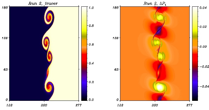
Figure 1: Subsonic regime (Run 2). The tracer and the ion pressure anisotropy, left and right frame respectively, at $t=375$.

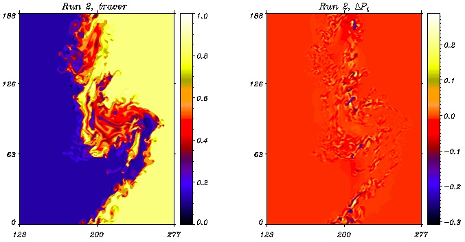
Figure 2: Subsonic regime (Run 2). The tracer and the ion pressure anisotropy, left and right frame respectively, at $t=670$

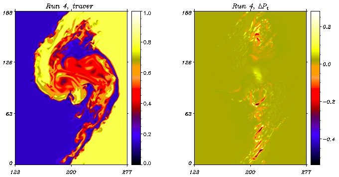
Figure 3: Intermediate regime (Run 4). The tracer and the ion pressure anisotropy, left and right frame respectively, at $t=540$

The pressure anisotropy grows in absolute value in correspondence to the compressed or rarefied regions. Plasma rarefaction occurs mainly inside the vortices during their formation, see Refs. miura:compressible ; palermo , while compression is mainly observed around the vortices in the form of a ribbon structure (surrounded by thin strips of rarefied plasma) or in between the vortices. In the same regions the magnetic field is also strongly reduced because of the plasma expansion or enhanced because of plasma compression thus affecting the value of $\Delta\beta_{anis}$, see Eq. (14). Depending on the nature of the density variation, rarefaction or compression, the sign of the pressure anisotropy, and thus of $\Delta\beta_{anis}$, will be either positive or negative thus selecting the possible further secondary instability, a firehose or a mirror instability, respectively: in the case of a rarefaction, $p_{\alpha\perp}$ becomes smaller than $p_{\alpha\|}$, corresponding to a positive $\Delta\beta$, see Eq. (14) while n the case of a compression, $p_{\alpha\perp}$ becomes larger than $p_{\alpha\|}$, corresponding to a negative $\Delta\beta_{anis}$.

In Fig. 2 we show the same quantities as in Fig. 1 at the later time $t=670$, when the pairing mechanism has generated one large big vortex corresponding to the largest size allowed by the numerical domain. The final vortex is characterized by a boundary profile dominated by small scale structures and filaments, see left frame, resulting from the development of local secondary instabilities. In the right frame, we see that the ion pressure anisotropy peaks inside several ion-scale structures along the boundary. These structures are relatively stable, are advected by the flow and maintain their own anisotropy. Except for these very localized structures, the ion pressure anisotropy is approximately negligible elsewhere.

The capability of the system to generate plasma anisotropy by rarefaction or compression increases at larger flow velocities, for instance at $U_{{}_{0}}=4$ and $U_{{}_{0}}=6$ (see Table 1). In Fig. 3 and in Fig. 4 (left and middle frame) we show the same quantities as in the previous figures during the non-linear regime long after saturation for Run 4 and Run 6. These runs correspond to an intermediate and to a supermagnetosonic regime, respectively. As discussed in Ref. palermo , at such values of the mean flow velocity $U_{{}_{0}}$ there is a transition towards the supermagnetosonic regime. The formation of shock structures is the main signature of this transition. Shocks cannot be observed in the tracer distribution but are clearly visible in the ion pressure anisotropy (see Fig. 4 middle frame) as well as in the other plasma quantities (not shown here) both on the left and on the right side of the vortices. Aside for the shock formation, the main difference with respect to the subsonic regime is that the development of secondary instabilities becomes increasingly ineffective and that extended regions are formed where the plasma is either rarefied or compressed (both in terms of the fluid and of the magnetic pressure) in particular inside the vortices or at their boundaries. Most of the plasma anisotropy is generated inside these regions.

In Fig. 4, right frame, we show the shaded iso-contours of the ratio between the in-plane and the out-plane magnetic field component for the supermagnetosonic regime, Run 6. We see that significant local increases of the in-plane magnetic field are produced inside the regions where the plasma is stretched and compressed while in the vortex central region, where we observe the formation of ion (and electron) pressure anisotropy (see, e.g., same figure, middle frame), the in-plane magnetic field remains very small. This is particularly relevant concerning the validity of the “eTF model” applied to the process of anisotropy generation since the model is obtained in the limit of a magnetic field perpendicular to the plane of the dynamics. This point will be further discussed in the following.

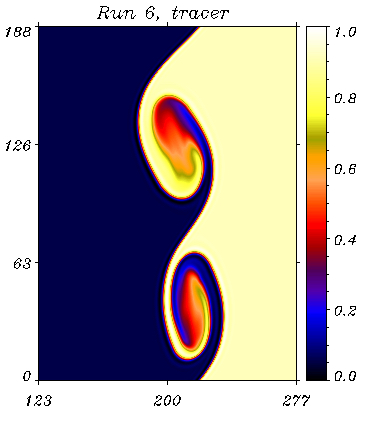
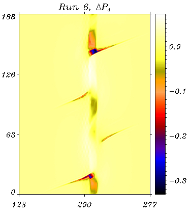
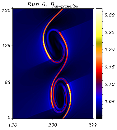
Figure 4: supermagnetosonic regime (Run 6). The tracer, the ion pressure anisotropy and the ratio between the in-plane and out-plane magnetic field, left, central and right frame respectively, at $t=374$

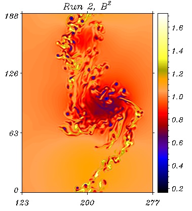
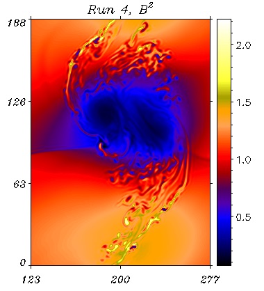
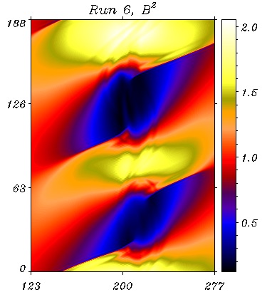
Figure 5: The magnetic pressure for the subsonic ($t=660$), intermediate ($t=520$), supermagnetosonic ($t=374$) regime, Run 2, 4, 6, left, middle and right frame, respectively

In order to stress the importance of the expansion/compression process associated with the vortex formation, in Fig. 5 we show the square of the magnetic field amplitude $B^{2}$ for the subsonic, the intermediate and the supermagnetosonic regimes, Run 2, 4 and 6, respectively, at the end of the saturated phase. The magnetic pressure ($\propto B^{2}$) is a direct signature of the plasma compression. By comparing these two pictures with the left frame of Fig. 2, 3 and 4, we see, as already discussed, that the vortices correspond to the regions of plasma rarefaction while the plasma is compressed in between. Quantitatively, the maximum (minimum) vortex rarefaction/compression values are comparable. This expansion/compression effect increases as we move towards the supermagnetosonic regime as the extension of the expanded/ compressed region increases. In the subsonic regime where secondary instabilities develop very efficiently, the peak values of plasma expansion/ compression are reached mainly inside small scale structures or at the vortex edges, (see Fig. 5, left frame). On the contrary in the intermediate and supermagnetosonic regimes the plasma becomes strongly rarefied all over the vortex region and compressed in between the vortices, as shown in Fig. 5, middle and right frame, respectively.

In Fig. 6 we show the shaded iso-contours of $\Delta\beta_{anis}$ as defined in Eq.(14) for the three regimes, Run 2, 4 and 6, respectively. We see that the dynamics naturally lead to configurations characterized by the presence in the central region of relatively strong $\beta$-anisotropy values that increase as the flow intensity increases. Both positive and negative values of $\Delta\beta_{anis}$ are produced which, in principle, could drive the plasma towards the development of the firehose or of the mirror instability. However in the subsonic regime the plasma anisotropy is limited to small regions so that a transition to a $\Delta\beta_{anis}$ unstable dynamics is unlikely. On the other hand in the intermediate and supermagnetosonic regimes $\Delta\beta_{anis}$ can become large over relatively extended regions so that a transition towards a firehose or mirror unstable dynamics is expected in these regimes.

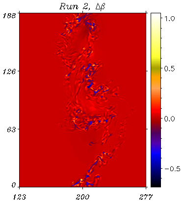
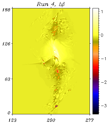
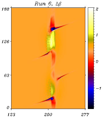
Figure 6: The plasma anisotropy as defined in Eq. (14) for the subsonic ($t=660$), intermediate ($t=520$), supermagnetosonic ($t=374$) regime, Run 2, 4, 6, left, middle and right frame, respectively

We see that these simulation results indicate that the nonlinear evolution of the KHI in the intermediate and supermagnetosonic regime can produce positive anisotropy values close to the firehose threshold and that, in addition, this anisotropy continues to increase with time. However, the 2D configuration assumed in the present investigation does not permit a correct study of the transition to a firehose unstable regime and thus it would be incorrect to continue the analysis of the plasma evolution after this threshold is reached. A similar argument holds for the negative anisotropy values where it would be incorrect even to refer to an instability threshold since the mirror instability must be addressed by using a kinetic model.

V.2 Exact Guide field regime

In Sec.V.1 we have studied the process of plasma anisotropy generation in the presence of an initial magnetic field at a small angle $\theta$ as defined in Eq.(10). This corresponds to a guide magnetic field directed along $z$ with a small in-plane component parallel to the flow, a typical configuration adopted in order to investigate the problem of the LLBL formation at the Magnetopause. In this case, if the mean magnetic field angle remains relatively small we can assume that the “eTF model” ext_two-fluid_model used here is still valid. However, as already discussed, the dynamics of the vortex chain generated by the K-H instability advects the in-plane magnetic field producing regions where the magnetic field is locally amplified as for example nearby the vortex boundaries or in between two vortices undergoing pairing. Nevertheless, the region where the “eTF model” might fail, in the sense that the mean magnetic field is no longer “almost perpendicular” to the plane of the dynamics, is mostly limited to the vortex ribbons while inside the vortices, where the anisotropy generation mechanism is the more efficient, the in-plane magnetic field remains small or even negligible.

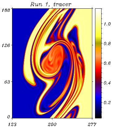
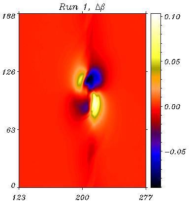
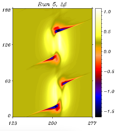
Figure 7: The strictly perpendicular magnetic field case. First two frames: the tracer, subsonic and supermagnetosonic regime, Run 1 and 5, respectively. Last two frames: the plasma anisotropy, subsonic and supermagnetosonic regime, Run 1 and 5, respectively.

In order to prove that the anisotropy generation is not an artifact of the model being pushed towards magnetic configurations that are not non strictly perpendicular, we have performed three runs, Run 1, 3 and 5, identical to the previous ones, but initializing the system with a strictly perpendicular magnetic field (see Table 1). In Fig. 7 we show the shaded iso-contours of the tracer, first two frames and of $\Delta\beta_{anis}$, last two frames for Run 1 and 5, respectively. The most important result is that in the supermagnetosonic regime, run 5, the efficiency of the plasma in generating plasma anisotropy, see Fig. 7 last frame, is approximately the same as in the case with an initial small in-plane magnetic field, run 6, discussed in Sec.V.1. This is due to the fact that two robust vortices are generated by the KHI where plasma anisotropy is efficiently produced. A similar behavior is qualitatively and quantitatively observed in the intermediate regime, run 3 (for the sake of brevity not shown here). On the other hand, a significant difference is observed in the subsonic regime where the plasma is now much less prone to the onset of secondary instabilities and in particular of magnetic reconnection (see Fig. 7, first frame). As a consequence, no small scale structures are generated which are the regions where in the non strictly perpendicular case, run 2, the anisotropy peaks are observed.

VI Conclusions

The generation of pressure anisotropy during the nonlinear evolution of a low collisionality plasma is being increasingly considered as a key dynamical player in space plasma systems, first of all in the heliosphere, but also in astrophysical systems as, e.g., (hot) accretion disks or galaxy clusters as well as in laboratory systems e.g., in the context of magnetic reconnection. In particular, distribution functions with different thermal pressure in the direction parallel or perpendicular to the magnetic field are today routinely detected in the solar wind. Moreover, structures emerging from the development of anisotropy instabilities such as, e.g. mirror modes, are also often observed in the solar wind. Recently, a strong theoretical and observational debate has occurred about the role of the firehose and mirror instability (using by the parallel plasma $\beta$) in constraining the formation of solar wind proton temperature anisotropy. In fact, pressure anisotropy is an important free energy source for relatively fast micro-instabilities that in turn can have a strong impact on the global structuring of the magnetic field or even on the shaping of the full system.

A series of different mechanisms, involving energy transfer between the parallel and the perpendicular direction, or preferential energy input from an external source or energy loss e.g., due to cyclotron emission, can induce pressure anisotropy in a low collisionality plasma. Here we have shown that the nonlinear dynamics of a vortex chain resulting from the development of the Kelvin Helmholtz instability driven by a sheared flow close to, or in, the supermagnetosonic regime, can produce a significant pressure anisotropy. This result is obtained by integrating numerically, in a two dimensional plasma configuration, a (two-fluid) dynamical model that includes a pressure tensor evolution equation explicitly. The resulting anisotropy is localized in the flow shear region. Pressure anisotropy, depending on its sign, can lead to the onset either of the mirror or of the firehose instability. The physical mechanism that causes such an anisotropy consists of two main steps:

$i$) first, the nonlinear evolution of the KH vortices compresses the plasma at the vortex boundaries and between them and expands it inside the vortices,

$ii$) then, the difference between the parallel and the perpendicular polytropic indices in the pressure tensor equation leads to a different variation of the parallel and of the perpendicular pressure tensor components even in the case of an initially isotropic pressure.

These results concerning the spontaneous formation of pressure anisotropy and the onset of anisotropy instabilities, such as the firehose or mirror instabilities, open up different possible scenarios in the nonlinear evolution of collisionless plasmas kunz2014 . In particular, not only the presence of pressure anisotropy can affect the KH dynamics Prajapati2010 , but also an early development of secondary instabilities driven by pressure anisotropy may compete with the magnetofluid timescale of the vortex dynamics, potentially becoming the dominant process at the later stage of the nonlinear evolution. Many configurations where shear flow instabilities develop have been outlined in the literature. First of all, let us underline that direct signatures about the role of the KHI as a primary drive for secondary mechanisms leading to temperature anisotropy have been detected in the plasma sheet in the near-Earth magnetosphere by satellite observations NishinoAnnGeo2007 and that the relevance of shear flow configurations for anisotropy-driven instabilities has been outlined also at the heliopause KuznetsovAL1995 . Furthermore, signatures indicating a possible development of a KHI have been observed in some merging galaxy groups RoedigerApJ2012 and at the sloshing cold fronts of some galaxy clusters RoedigerApJ2013 . Velocity shear instabilities are indicated also to play a role between the hot intracluster gas and the moving galaxies where turbulent layers could be generated RoedigerMNRAS2013 . Finally, we note that anisotropy pressure development can play an important role also on the context of magnetic reconnection by, e.g. changing the symmetry of the system significantly and modifying the magnetic field configuration Cassak2015 . Therefore, the KHI and its associated secondary instabilities including pressure anisotropy instabilities, may provide a relevant mechanism for the dynamics and the generation of turbulent layers in many different environments, not limited to the LLBL magnetosphere case.

We conclude by noticing that this analysis must be considered as a first step towards a full 3D kinetic treatment that has been adopted for t he sake of mathematical and computational simplicity. Indeed, the present analysis is on the one hand well suited to identify the onset of such a mechanism of anisotropy generation but, on the other hand, it cannot predict accurately its evolution once the firehose or mirror instability threshold is approaching, first of all because of the 2D configuration. We nevertheless underline that even within these limitations, our analysis is relevant to asses that shear flows in space and, more generally in collisionless magnetized plasmas, are an important energy source for the development of anisotropy instabilities at play during the further nonlinear dynamics.

- (1) Miura A.1984, J. Geophys. Res. 89, 801
- (2) Ohtani S. et al. 1999, Journal of Geophysics Research 104, A22381
- (3) Otto A., Fairfield D.H. 2000, Journal of Geophysics Research 105, A921175
- (4) Hasegawa H. et al. 2004, Nature 430, 755
- (5) Fairfield D.H. et al. 2000, J. Geophys. Res. [Space Phys.] 105, 21159
- (6) Foullon C. et al. 2008, J. Geophys. Res. 113, A11203
- (7) Phan T.D. et al. 2000, Nature 404(20), 848
- (8) Terasawa T. et al. 1997, Geophysics Research Letters 24-8, 935-938
- (9) M. Fujimoto et al. 1998, J. Geophys. Res. 103, 4391
- (10) Liu Z.X., Hu Y.D. 1988, Geophys. Res. Lett. 15, 752
- (11) Nakamura T.K., Fujimoto M. 2005, Geophys. Res. Lett. 32, L21102
- (12) Faganello M., Califano F., Pegoraro F. 2008, Physical Rev. Lett. 101, 175003
- (13) Smyth W. D. 2003, J. Fluid Mech. 497, 67
- (14) Matsumoto Y., Hoshino M. 2004, Geophys. Res. Lett. 31, L02807
- (15) Faganello M., Califano F., Pegoraro F. 2008, Physical Review Letters 100, 015001
- (16) Tenerani A., Faganello M., Califano F., Pegoraro F. 2011, Plasma Phys. Controlled Fusion 53, 015003
- (17) Henri P., Califano F., Faganello M., Pegoraro F. 2012, Physics of Plasmas 19, 072908
- (18) Rosenbluth M.N., Krall N.A., Rostoker N. 1962, Nucl. Fusion Suppl. Pt. 1, 143
- (19) Roberts K.V., J.B. Taylor J.B. 1962, Phys. Rev. Lett. 8, 197
- (20) Snyder P.B., Hammett G.W., Dorland B. 1997, Physics of Plasmas 4, 3974
- (21) Kunz M.W. et al. 2015, J. of Plasma Physics 81-05, 325810501
- (22) Passot P., Sulem P.L. 2007, Physics of Plasmas 14, 082502
- (23) H. Karimabadi et al. 2013, Physics of Plasmas 20, 012303
- (24) Cerri S.S. et al. 2014, Physics of Plasmas 21, 112109
- (25) Cerri S.S. et al. 2014, Physics of Plasmas 20, 112112
- (26) Chew G.F., Goldberger M.L., Low F.E. 1956, Royal Society of London Proceedings Series A 236, 112
- (27) Faganello M., Califano F., Pegoraro F. 2009, New Journal of Physics 11, 063008
- (28) F. Palermo et al. 2011, Journal of Geophysics Research 116, A04223
- (29) Miura A. 1997, Physics of Plasmas 4, 2871
- (30) Palermo F., Faganello M., Califano F., Pegoraro F. 2011, Annales Geophysicae 29, 020705
- (31) W. Kunz, A. Schekochihin, J. Stone 2014, Phys. Rev. Lett. 112, 205003
- (32) R. P. Prajapati, R. K. Chhajlani 2010, Physics of Plasmas 17, 112108
- (33) Nishino M. N., Fujimoto M., Ueno G., Mukai T., Saito Y. 2007, Ann. Geophys. 25, 2069
- (34) Kuznetsov V. D., Nakaryakov V. M., Tsyganov P. V. 1995, Astronomy Letters 21, 710
- (35) Roediger E., Kraft R. P., Machacek M. E., Forman W. R., Nulsen P. E. J., Jones C., Murray S. S. 2012, Astrophys. J. 754, 147
- (36) Roediger E., Kraft R. P., Forman W. R., Nulsen P. E. J., Churazov E. 2013, Astrophys. J. 764, 60
- (37) Roediger E., Kraft R. P., Nulsen P., Churazov E., Forman W., Brüggen M., Kokotanekova R. 2013, Mon. Not. R. Astron. Soc. 436, 1721
- (38) P. A. Cassak et al. 2015, Physics of Plasmas 22, 020705