Stabilised finite element methods for ill-posed problems with conditional stability

Abstract

In this paper we discuss the adjoint stabilised finite element method introduced in E. Burman, Stabilized finite element methods for nonsymmetric, noncoercive and ill-posed problems. Part I: elliptic equations, SIAM Journal on Scientific Computing Bu13 and how it may be used for the computation of solutions to problems for which the standard stability theory given by the Lax-Milgram Lemma or the Babuska-Brezzi Theorem fails. We pay particular attention to ill-posed problems that have some conditional stability property and prove (conditional) error estimates in an abstract framework. As a model problem we consider the elliptic Cauchy problem and provide a complete numerical analysis for this case. Some numerical examples are given to illustrate the theory.

1 Introduction

Most methods in numerical analysis are designed making explicit use of the well-posedness Hada02 of the underlying continuous problem. This is natural as long as the problem at hand indeed is well-posed, but even for well-posed continuous problems the resulting discrete problem may be unstable if the finite element spaces are not well chosen or if the mesh-size is not small enough. This is for instance the case for indefinite problems, such as the Helmholtz problem, or constrained problems such as Stokes’ equations. For problems that are ill-posed on the continuous level on the other hand the approach makes less sense and leads to the need of regularization on the continuous level so that the ill-posed problem can be approximated by solving a sequence of well-posed problems. The regularization of the continuous problem can consist for example of Tikhonov regularization TA77 or a so-called quasi reversibility method LL69 . In both cases the underlying problem is perturbed and the original solution (if it exists) is recovered only in the limit as some regularization parameter goes to zero. The disadvantage of this approach from a numerical analysis perspective is that once the continuous problem has been perturbed to some order, the accuracy of the computational method must be made to match that of the regularization. The strength of the regularization on the other hand must make the continuous problem stable and damp perturbations induced by errors in measurement data. This leads to a twofold matching problem where the regularization introduces a perturbation of first order, essentially excluding the efficient use of many tools from numerical analysis such as high order methods, adaptivity and stabilisation. The situation is vaguely reminiscent of that in conservation laws where in the beginning low order methods inspired by viscosity solution arguments dominated, to later give way for high resolution techniques, based on flux limiter finite volume schemes or (weakly) consistent stabilised finite element methods such as the Galerkin Least Squares methods (GaLS) or discontinuous Galerkin methods (dG) (see for instance CJST98 and references therein). These methods allow for high resolution in the smooth zone while introducing sufficient viscous stabilisation in zones with nonlinear phenomena such as shocks or rarefaction waves.

In this paper our aim is to advocate a similar shift towards weakly consistent stabilisation methods for the computation of ill-posed problems. The philosophy behind this is to cast the problem in the form of a constrained optimisation problem, that is first discretized, leading to a possibly unstable discrete problem. The problem is then regularized on the discrete level using techniques known from the theory of stabilised finite element methods. This approach has the following potential advantages some of which will be explored below:

• the optimal scaling of the penalty parameter with respect to the mesh parameter follows from the error analysis;

• for ill-posed problems where a conditional stability estimate holds, error estimates may be derived that are in a certain sense optimal with respect to the discretization parameters;

• discretization errors and perturbation errors may be handled in the same framework;

• a posteriori error estimates may be used to drive adaptivity;

• a range of stabilised finite element methods may be used for the regularization of the discrete problem;

• the theory can be adapted to many different problems.

Stabilised finite element methods represent a general technique for the regularization of the standard Galerkin method in order to improve its stability properties for instance for advection–diffusion problems at high Péclet number or to achieve inf-sup stability for the pressure-velocity coupling in the Stokes’ system. To achieve optimal order convergence the stabilisation terms must have some consistency properties, i.e. they decrease at a sufficiently high rate when applied to the exact solution or to any smooth enough function. Such stabilising terms appear to have much in common with Tikhonov regularization in inverse problems, although the connection does not seem to have been made in general. In the recent papers Bu13 ; Bu14a we considered stabilised finite element methods for problems where coercivity fails for the continuous problem and showed that optimal error estimates can be obtained without, or under very weak, conditions on the physical parameters and the mesh parameters, also for problems where the standard Galerkin method may fail.

In the first part of this series Bu13 we considered the analysis of elliptic problems without coercivity using duality arguments. The second part Bu14a was consecrated to problems for which coercivity fails, but which satisfy the Babuska-Brezzi Theorem, illustrated by the transport equation. Finally in the note Bu14b we extended the analysis of Bu13 to the case of ill-posed problems with some conditional stability property.

Our aim in the present essay is to review and unify some of these results and give some further examples of how stabilised methods can be used for the solution of ill-posed problem. To exemplify the theory we will restrict the discussion to the case of scalar second order elliptic problems on the form

$$\mathcal{L}u=f\quad\mbox{ in }\Omega$$ (1)

where $\mathcal{L}$ is a linear second order elliptic operator, $u$ is the unknown and $f$ is some known data and $\Omega$ is some simply connected, open subset of $\mathbb{R}^{d}$, $d=2,3$. Observe that the operator $\mathcal{L}$ does not necessarily have to be on divergence form, although we will only consider this case here to make the exposition concise (see WaWa15 for an analysis of well-posed elliptic problems on nondivergence form).

The discussion below will also be restricted to finite element spaces that are subsets of $H^{1}(\Omega)$. For the extension of these results to a nonconforming finite element method we refer to Bu14c .

1.1 Conditional stability for ill-posed problems

There is a rich literature on conditional stability estimates for ill-posed problems. Such estimates often take the form of three sphere’s inequalities or Carleman estimates, we refer the reader to ARRV09 and references therein.

The estimates are conditional, in the sense that they only hold under the condition that the exact solution exists in some Sobolev space $V$, equipped with scalar product $(\cdot,\cdot)_{V}$ and associated norm $\|\cdot\|_{V}:=(\cdot,\cdot)_{V}$. Hereinwe will only consider the case where $V\equiv H^{1}(\Omega)$. Then we introduce $V_{0}\subset V$ and consider the problem: find $u\in V_{0}$ such that

$$a(u,w)=l(w),\quad\forall w\in W,$$ (2)

Observe that $V_{0}$ and $W$ typically are different subsets of $H^{1}(\Omega)$ and we do not assume that $W$ is a subset or $V_{0}$ or vice versa. The operators $a(\cdot,\cdot):V\times V\rightarrow\mathbb{R},\,l(\cdot):W\rightarrow\mathbb{R}$ denote a bounded bilinear and a bounded linear form respectively. The form $a(\cdot,\cdot)$ is a weak form of $\mathcal{L}u$. We let $\|\cdot\|_{C}$ denote the norm for which the condition must be satisfied and $\|\cdot\|_{S}$ denote the norm in which the stability holds.

We then assume that a stability estimate of the following form holds: if for some $x\in V_{0}$, with $\|x\|_{C}\leq E$ there exist $\varepsilon<1$ and $r\in W^{\prime}$ such that

$$\begin{array}[]{cc}\left\{\begin{array}[]{l}a(x,v)=(r,v)_{\left<W^{\prime},W\right>}\;\forall v\in W\\ \|r\|_{W^{\prime}}\leq\varepsilon\end{array}\right.;&\quad\mbox{ then }\|x\|_{S}\leq\Xi_{E}(\varepsilon),\end{array}$$ (3)

where $\Xi_{E}(\cdot):\mathbb{R}^{+}\rightarrow\mathbb{R}^{+}$ is a smooth, positive, function, depending on the problem, $\|\cdot\|_{S}$ and $E$, with $\lim_{s\rightarrow 0ˆ+}\Xi_{E}(s)=0$. Depending on the problem different smallness conditions may be required to hold on $\varepsilon$.

The idea is that the stabilised methods we propose may use the estimate (3) directly for the derivation of error estimates, without relying on the Lax-Milgram Lemma or the Babuska-Brezzi Theorem. Let us first make two observations valid also for well-posed problems. When the assumptions of the Lax-Milgram’s lemma are satisifed (3) holds unconditionally for the energy norm and $\Xi_{E}(\varepsilon)=C\varepsilon$, for some problem dependent constant $C$. If for a given problem the adjoint equation $a(v,z)=j(v)$ admits a solution $z\in W$, with $\|z\|_{W}\leq E_{j}$, for some linear functional $j\in V^{\prime}$ then

$$|j(x)|=|a(x,z)|=|r(z)|\leq E_{j}\|r\|_{W^{\prime}}$$ (4)

and we see that for this case the condition of the conditional stability applies to the adjoint solution.

Herein we will focus on the case of the elliptic Cauchy problem as presented in ARRV09 . In this problem both Dirichlet and Neumann data are given on a part of the boundary, whereas nothing is known on the complement. We will end this section by detailing the conditional stability (3) of the elliptic Cauchy problem. We give the result here with reduced technical detail and refer to ARRV09 for the exact dependencies of the constants on the physical parameters and the geometry.

1.2 Example: the elliptic Cauchy problem

The problem that we are interested in takes the form

$$\left\{\begin{array}[]{rcl}-\nabla\cdot(\sigma\nabla u)+cu&=&f,\mbox{ in }\Omega\\ u&=&0\mbox{ on }\Gamma_{D}\\ \partial_{n}u&=&\psi\mbox{ on }\Gamma_{N}\end{array}\right.$$ (5)

where $\Omega\subset\mathbb{R}^{d}$, $d=2,3$ is a polyhedral (polygonal) domain with boundary $\partial\Omega$, $\partial_{n}u:=n^{T}\cdot\nabla u$, (with $n$ the outward pointing normal on $\partial\Omega$), $\sigma\in\mathbb{R}^{d\times d}$ is a symmetric matrix for which $\exists\sigma_{0}\in\mathbb{R}$, $\sigma_{0}>0$ such that $y^{T}\cdot\sigma y>\sigma_{0}$ for all $y\in\mathbb{R}^{d}$ and $c\in\mathbb{R}$. By $\Gamma_{N},\,\Gamma_{D}$ we denote polygonal subsets of the boundary $\partial\Omega$, with union $\Gamma_{B}:=\Gamma_{D}\cup\Gamma_{N}$ and that overlap on some set of nonzero $(d-1)$-dimensional measure, $\Gamma_{S}:=\Gamma_{D}\cap\Gamma_{N}\neq\emptyset$. We denote the complement of the Dirichlet boundary $\Gamma_{D}^{\prime}:=\partial\Omega\setminus\Gamma_{D}$, the complement of the Neumann boundary $\Gamma_{N}^{\prime}:=\partial\Omega\setminus\Gamma_{N}$ and the complement of their union $\Gamma_{B}^{\prime}:=\partial\Omega\setminus\Gamma_{B}$. To exclude the well-posed case, we assume that the $(d-1)$-dimensional measure of $\Gamma_{S}$ and $\Gamma_{B}^{\prime}$ is non-zero. The practical interest in (5) stems from engineering problems where the boundary condition, or its data, is unknown on $\Gamma_{B}^{\prime}$, but additional measurements $\psi$ of the fluxes are available on a part of the accessible boundary $\Gamma_{S}$. This results in an ill-posed reconstruction problem, that in practice most likely does not have a solution due to measurement errors in the fluxes Belg07 . However if the underlying physical process is stable, (in the sense that the problem where boundary data is known is well-posed) we may assume that it allows for a unique solution in the idealized situation of unperturbed data. This is the approach we will take below. To this end we assume that $f\in L^{2}(\Omega)$, $\psi\in L^{2}(\Gamma_{N})$ and that a unique $u\in H^{s}(\Omega)$, $s>\tfrac{3}{2}$ satisfies (5). For the derivation of a weak formulation we introduce the spaces $V_{0}:=\{v\in H^{1}(\Omega):v|_{\Gamma_{D}}=0\}$ and $W:=\{v\in H^{1}(\Omega):v|_{\Gamma_{N}^{\prime}}=0\},$ both equipped with the $H^{1}$-norm and with dual spaces denoted by $V_{0}^{\prime}$ and $W^{\prime}$.

Using these spaces we obtain a weak formulation: find $u\in V_{0}$ such that

$$a(u,w)=l(w)\quad\forall w\in W,$$ (6)

where

$$a(u,w)=\int_{\Omega}(\sigma\nabla u)\cdot\nabla w+cuw~{}\mbox{d}x,$$

and

$$l(w):=\int_{\Omega}fw~{}\mbox{d}x+\int_{\Gamma_{N}}\psi\,w~{}\mbox{d}s.$$

It is known (ARRV09, , Theorems 1.7 and 1.9 with Remark 1.8) that if there exists a solution $u\in H^{1}(\Omega)$, to (6), a conditional stability of the form (3) holds provided $0\leq\varepsilon<1$ and

$$\begin{array}[]{l}\mbox{$\|u\|_{S}:=\|u\|_{L^{2}(\omega)}$, $\omega\subset\Omega:\,\mbox{dist}(\omega,\Gamma_{B}^{\prime})=:d_{\omega,\Gamma_{B}^{\prime}}>0$}\\[8.53581pt] \mbox{ with $\Xi(\varepsilon)=C(E)\varepsilon^{\tau}$, $C(E)>0$, $\tau:=\tau(d_{\omega,\Gamma_{B}^{\prime}})\in(0,1),\,E=\|u\|_{L^{2}(\Omega)}$}\end{array}$$ (7)

and for

$$\begin{array}[]{l}\mbox{$\|u\|_{S}:=\|u\|_{L^{2}(\Omega)}$ with $\Xi(\varepsilon)=C_{1}(E)(|\log(\varepsilon)|+C_{2}(E))^{-\tau}$}\\[8.53581pt] \mbox{ with $C_{1}(E),C_{2}(E)>0$, $\tau\in(0,1),\,E=\|u\|_{H^{1}(\Omega)}.$}\end{array}$$ (8)

How to design accurate computational methods that can fully exploit the power of conditional stability estimates for their analysis remains a challenging problem. Nevertheless the elliptic Cauchy problem is particularly well studied. For pioneering work using logarithmic estimates we refer to FM86 ; RHD99 and quasi reversibility KS91 . For work using regularization and/or energy minimisation see ABF06 ; ABB06 ; CN06 ; HHKC07 ; HLT11 . Recently progress has been made using least squares DHH13 or quasi reversibility approaches Bour05 ; Bour06 ; BD10a inspired by conditional stability estimates BD10b . In this paper we draw on our experiences from Bu14b ; Bu14c , that appear to be the first works where error estimates for stabilised finite element methods on unstructured meshes have been derived for this type of problem. For simplicity we will only consider the operator $\mathcal{L}u:=-\Delta u+cu$, with $c\in\mathbb{R}$ for the discussion below.

2 Discretization of the ill-posed problem

We will here focus on discretizations using finite element spaces, but the ideas in this section are general and may be applied to any finite dimensional space.

We consider the setting of section 1.2. Let $\{\mathcal{T}_{h}\}_{h}$ denote a family of quasi uniform, shape regular simplicial triangulations, $\mathcal{T}_{h}:=\{K\}$, of $\Omega$, indexed by the maximum simplex diameter $h$. The set of faces of the triangulation will be denoted by $\mathcal{F}$ and $\mathcal{F}_{I}$ denotes the subset of interior faces. The unit normal of a face of the mesh will be denoted $n$, its orientation is arbitrary but fixed, except on faces in $\partial\Omega$ where the normal is chosen to point outwards from $\Omega$. Now let $X_{h}^{k}$ denote the finite element space of continuous, piecewise polynomial functions on $\mathcal{T}_{h}$,

$$X_{h}^{k}:=\{v_{h}\in H^{1}(\Omega):v_{h}|_{K}\in\mathbb{P}_{k}(K),\quad\forall K\in\mathcal{T}_{h}\}.$$

Here $\mathbb{P}_{k}(K)$ denotes the space of polynomials of degree less than or equal to $k$ on a simplex $K$. Letting $(\cdot,\cdot)_{X}$ denote the $L^{2}$-scalar product over $X\subset\mathbb{R}^{d}$ and $\left<\cdot,\cdot\right>_{X}$ that over $X\subset\mathbb{R}^{d-1}$, with associated $L^{2}$-norms $\|\cdot\|_{X}$, we define the broken scalar products and the associated norms by,

$$(u_{h},v_{h})_{h}:=\sum_{K\in\mathcal{T}_{h}}(u_{h},v_{h})_{K},\quad\|u_{h}\|_{h}:=(u_{h},u_{h})_{h}^{\frac{1}{2}},$$

$$\left<u_{h},v_{h}\right>_{\mathcal{F}}:=\sum_{F\in\mathcal{F}}\left<u_{h},v_{h}\right>_{F},\quad\|u_{h}\|_{\mathcal{F}}:=\left<u_{h},u_{h}\right>_{\mathcal{F}}^{\frac{1}{2}}.$$

If we consider finite dimensional subspaces $V_{h}\subset V_{0}$ and $W_{h}\subset W$, for instance in the finite element context we may take $V_{h}:=X_{h}^{k}\cap V_{0}$ and $W_{h}:=X_{h}^{k}\cap W$, the discrete equivalent of problem (2) (with $g=0$) reads: find $u_{h}:=\sum_{j=1}^{N_{V_{h}}}u_{j}\varphi_{j}\in V_{h}$ such that

$$a(u_{h},\phi_{i})=l(\phi_{i}),\quad i=1,\ldots,N_{W_{h}}$$ (9)

where the $\{\varphi_{i}\}$ and $\{\phi_{i}\}$ are suitable bases for $V_{h}$ and $W_{h}$ respectively and $N_{V_{h}}:=\mbox{dim}(V_{h})$, $N_{W_{h}}:=\mbox{dim}(W_{h})$ This formulation may be written as the linear system

$$AU=L,$$

where $A$ is an $N_{W_{h}}\times N_{V_{h}}$ matrix, with coefficients $A_{ij}:=a(\varphi_{j},\phi_{i})$, $U=(u_{1},\ldots,u_{N_{V}})^{T}$ and $L=(l(\phi_{1}),\ldots,l(\phi_{N_{W_{h}}}))^{T}$. Observe that since we have not assumed $N_{V_{h}}=N_{W_{h}}$ this system may not be square, but even if it is, it may have zero eigenvalues. This implies

1. non-uniqueness: there exists $\tilde{U}\in\mathbb{R}^{N_{V_{h}}}\setminus\{{\boldmath{0}}\}$ such that $A\tilde{U}=0$;

2. non-existence: there exists $L\in\mathbb{R}^{N_{V_{h}}}$ such that $L\not\in\mbox{Im}(A)$.

These two problems actually appear also when discretizing well-posed continuous models. Consider the Stokes’ equation for incompressible elasticity, for this problem the well-known challenge is to design a method for which the pressure variable is stable and the velocity field discretely divergence free. Indeed the discrete spaces for pressures and velocities must be well-balanced. Otherwise, there may be spurious pressure modes in the solution, comparable to point 1. above, or if the pressure space is too rich the solution may “lock”, implying that only the zero velocity satisfies the divergence free constraint, which is comparable to 2. above. Drawing on the experience of the stabilisation of Stokes’ problem this analogy naturally suggests the following approach to the stabilisation of (9).

• Consider (9) of the form $a(u_{h},w_{h})=l(w_{h})$ as the constraint for a minimisation problem;

• minimise some (weakly) consistent stabilisation together with a penalty for the boundary conditions (or other data) under the constraint;

• stabilise the Lagrange multiplier (since discrete inf-sup stability fails in general).

To this end we introduce the Lagrangian functional:

$$\boxed{\L(u_{h},z_{h}):=\frac{1}{2}s_{V}(u_{h}-u,u_{h}-u)-\frac{1}{2}s_{W}(z_{h},z_{h})+a_{h}(u_{h},z_{h})-l_{h}(z_{h})}$$ (10)

where $s_{V}(u_{h}-u,u_{h}-u)$ and $s_{W}(z_{h},z_{h})$ represents a penalty term, imposing measured data through the presence of $s_{V}(u_{h}-u,u_{h}-u)$ and symmetric, weakly consistent stabilisations for the primal and adjoint problems respectively. The forms $a_{h}(\cdot,\cdot)$ and $l_{h}(\cdot)$ are discrete realisations of $a(\cdot,\cdot)$ and $l(\cdot)$, that may account for the nonconforming case where $V_{h}\not\subset V$ and $W_{h}\not\subset W$.

The discrete method that we propose is given by the Euler-Lagrange equations of (10), find $(u_{h},z_{h})\in V_{h}\times W_{h}$ such that

$$\begin{array}[]{rcl}a_{h}(u_{h},w_{h})-s_{W}(z_{h},w_{h})&=&l_{h}(w_{h})\\[8.53581pt] a_{h}(v_{h},z_{h})+s_{V}(u_{h},v_{h})&=&s_{V}(u,v_{h}),\end{array}$$ (11)

for all $(v_{h},w_{h})\in V_{h}\times W_{h}$. This results in a square linear system regardless of the dimensions of $V_{h}$ and $W_{h}$. Note the appearance of $s_{V}(u,v_{h})$ in the right hand side of the second equation of (11). This means only stabilisations for which $s_{V}(u,v_{h})$ can be expressed using known data may be used. This typically is the case for residual based stabilisations, but also allows for the inclusion of measured data in the computation in a natural fashion. The stabilising terms in (11) are used both to include measurements, boundary conditions and regularization. In order to separate these effects we will sometimes write

$$s_{x}(\cdot,\cdot):=s^{D}_{x}(\cdot,\cdot)+s^{S}_{x}(\cdot,\cdot),\quad x=V,W$$

where the $s^{D}$ contribution is associated with assimilation of data (boundary or measurements) and the $s^{S}$ contribution is associated with the stabilising terms. For the Cauchy problem $s^{D}_{V}(u,v_{h})$ depends on $\psi$ and $s^{S}_{V}(u,v_{h})$ may depend on $f$ as we shall see below.

Observe that the second equation of (11) is a finite element discretization of the dual problem associated to the pde-constraint of (10). Hence, assuming that a unique solution exists for the given data, the solution to approximate is $z=0$. The discrete function $z_{h}$ will most likely not be zero, since it is perturbed by the stabilisation operator acting on the solution $u_{h}$, which in general does not coincide with the stabilisation acting on $u$. The precise requirements on the forms will be given in the next section together with the error analysis. We also introduce the following compact form of the formulation (11), find $(u_{h},z_{h})\in V_{h}\times W_{h}$ such that

$$A_{h}[(u_{h},z_{h}),(v_{h},w_{h})]=L_{h}(v_{h},w_{h})\mbox{ for all }(v_{h},w_{h})\in V_{h}\times W_{h},$$ (12)

where

$$A_{h}[(u_{h},z_{h}),(v_{h},w_{h})]:=a_{h}(u_{h},w_{h})-s_{W}(z_{h},w_{h})+a_{h}(v_{h},z_{h})+s_{V}(u_{h},v_{h})$$ (13)

and

$$L_{h}(v_{h},w_{h}):=l_{h}(w_{h})+s_{V}(u,v_{h}).$$

We will end this section by giving some examples of the construction of the discrete forms. To reduce the amount of generic constants we introduce the notation $a\lesssim b$ for $a\leq Cb$ where $C$ denotes a positive constant independent of the mesh-size $h$.

2.1 Example: discrete bilinear forms and penalty terms for the elliptic Cauchy problem

For the elliptic Cauchy problem of section 1.2 we define $V^{k}_{h}$ and $W^{k}_{h}$ to be $X_{h}^{k}$ (the superscript will be dropped for general $k$). Then we use information on the boundary conditions to design a form $a_{h}(\cdot,\cdot)$ that is both forward and adjoint consistent. A penalty term is also added to enforce the boundary condition.

$$a_{h}(u_{h},v_{h}):=a(u_{h},v_{h})-\left<\partial_{n}u_{h},v_{h}\right>_{\Gamma_{N}^{\prime}}-\left<\partial_{n}v_{h},u_{h}\right>_{\Gamma_{D}}$$ (14)

$$s^{D}_{V}(u_{h},w_{h}):=\gamma_{D}\left<h^{-1}u_{h},w_{h}\right>_{\Gamma_{D}}+\gamma_{D}\left<h\partial_{n}u_{h},\partial_{n}w_{h}\right>_{\Gamma_{N}},$$ (15)

where $\gamma_{D}\in\mathbb{R}_{+}$ denotes a penalty parameter that for simplicity is taken to be the same for all the $s^{D}(\cdot,\cdot)$ terms, it follows that, if $u=g$ on $\Gamma_{D}$,

$$s^{D}_{V}(u,w_{h}):=\gamma_{D}\left<h^{-1}g,w_{h}\right>_{\Gamma_{D}}+\gamma_{D}\left<h\,\psi,\partial_{n}w_{h}\right>_{\Gamma_{N}}.$$

The adjoint boundary penalty may then be written

$$s^{D}_{W}(z_{h},v_{h}):=\gamma_{D}\left<h^{-1}z_{h},v_{h}\right>_{\Gamma_{N}^{\prime}}+\gamma_{D}\left<h\,\partial_{n}z_{h},\partial_{n}v_{h}\right>_{\Gamma_{D}^{\prime}}.$$ (16)

We assume that the computational mesh $\mathcal{T}_{h}$ is such that the boundary subdomains consist of the union of boundary element faces, i.e. the boundaries of $\Gamma_{D}$ and $\Gamma_{N}$ coincide with element edges. Finally we let $l_{h}(v_{h})$ coincide with $l(v_{h})$ for unperturbed data. Observe that there is much more freedom in the choice of the stabilisation for $z_{h}$ since the exact solution satisfies $z=0$. We will first discuss the methods so that they are consistent also in the case $z\neq 0$, in order to facilitate the connection to a larger class of control problems. Then we will suggest a stronger stabilisation for $z_{h}$.

2.2 Example: Galerkin Least Squares stabilisation

For the stabilisation term we first consider the classical Galerkin Least Squares stabilisation. Observe that for the finite element spaces considered herein, the GaLS stabilisation in the interior of the elements must be complemented with a jump contribution on the boundary of the element. If $C^{1}$-continuous approximation spaces are used this latter contribution may be dropped. First consider the least squares contribution,

$$s^{S}_{V}(u_{h},v_{h}):=\gamma_{S}(h^{2}\mathcal{L}u_{h},\mathcal{L}v_{h})_{h}+\gamma_{S}\left<h\llbracket\partial_{n}u_{h}\rrbracket,\llbracket\partial_{n}v_{h}\rrbracket\right>_{\mathcal{F}_{I}},\,\gamma_{S}\in\mathbb{R}_{+}.$$ (17)

Here $\llbracket\partial_{n}v_{h}\rrbracket$ denotes the jump of the normal derivative of $v_{h}$ over an element face $F$. It then follows that, considering sufficiently smooth solutions, $u\in H^{s}(\Omega)$, $s>3/2$,

$$s^{S}_{V}(u,v_{h}):=\gamma_{S}(h^{2}f,\mathcal{L}v_{h})_{h}.$$

Similarly we define

$$s^{S}_{W}(z_{h},w_{h})=\gamma_{S}(h^{2}\mathcal{L}^{*}z_{h},\mathcal{L}^{*}w_{h})_{h}+\gamma_{S}\left<h\llbracket\partial_{n}z_{h}\rrbracket,\llbracket\partial_{n}w_{h}\rrbracket\right>_{\mathcal{F}_{I}}.$$

For symmetric operators $\mathcal{L}$ we see that $s^{S}_{W}(\cdot,\cdot)\equiv s^{S}_{V}(\cdot,\cdot)$, however in the presence of nonsymmetric terms they must be evaluated separately.

2.3 Example: Continuous Interior Penalty stabilisation

In this case we may choose the two stabilisations to be the same, $s^{S}_{W}(\cdot,\cdot)\equiv s^{S}_{V}(\cdot,\cdot)$ and

$$s^{S}_{V}(u_{h},v_{h})=\gamma_{S}\left<h^{3}\llbracket\Delta u_{h}\rrbracket,\llbracket\Delta v_{h}\rrbracket\right>_{\mathcal{F}_{I}}+\gamma_{S}\left<h\llbracket\partial_{n}u_{h}\rrbracket,\llbracket\partial_{n}v_{h}\rrbracket\right>_{\mathcal{F}_{I}}.$$ (18)

2.4 Example: Stronger adjoint stabilisation

Observe that since the exact solution satisfies $z=0$ we can also use the adjoint stabilisation

$$s^{S}_{W}(z_{h},w_{h})=\gamma_{S}(\nabla z_{h},\nabla w_{h})_{\Omega}$$ (19)

This simplifies the formulation for non-symmetric problems when the GaLS method is used and reduces the stencil, but the resulting formulation is no longer adjoint consistent and optimal $L^{2}$-estimates may no longer be proved in the well-posed case (see Bu13 for a discussion). In this case the formulation corresponds to a weighted least squares method. This is easily seen by eliminating $z_{h}$ from the formulation (11).

2.5 Penalty parameters

Above we have introduced the penalty parameters $\gamma_{S}$ and $\gamma_{D}$. The size of these parameters play no essential role for the discussion below. Indeed the convergence orders for unperturbed data are obtained only under the assumption that $\gamma_{S},\gamma_{D}>0$. Therefore the explicit dependence of the constants in the estimates will not be tracked. Only in some key estimates, relating to stability and preturbed data, will we indicate the dependence on the parameters in terms of $\gamma_{min}:=\min(\gamma_{S},\gamma_{D})$ or $\gamma_{max}:=.\max(\gamma_{S},\gamma_{D})$.

3 Hypothesis on forms and interpolants

To prepare for the error analysis we here introduce assumptions on the bilinear forms. The key properties that are needed are a discrete stability estimate, that the form $a_{h}(\cdot,\cdot)$ is continuous on a norm that is controlled by the stabilisation terms and that the finite element residual can be controlled by the stabilisation terms. To simplify the presentation we will introduce the space $H^{s}(\Omega)$, with $s\in\mathbb{R}_{+}$ which corresponds to smoother functions than those in $V$ for which $a_{h}(u,v_{h})$ and $s_{V}(u,v_{h})$ always are well defined. This typically allows us to treat the data part $s_{V}^{D}$ and the stabilisation part $s_{V}^{S}$ together using strong consistency. A more detailed analysis separating the two contributions in $s_{V}$ and handling the conformity error of $a_{h}$ for $u\in V$ allows an analysis under weaker regularity assumptions.

Consistency:

If $u\in V\cap H^{s}(\Omega)$ is the solution of (1), then the following Galerkin orthogonality holds

$$a_{h}(u_{h}-u,w_{h})-s_{W}(z_{h},w_{h})=l_{h}(w_{h})-l(w_{h}),\quad\mbox{ for all }w_{h}\in W_{h}.$$ (20)

Stabilisation operators:

We consider positive semi-definite, symmetric stabilisation operators, $s_{V}:V_{h}\times V_{h}\mapsto\mathbb{R},\quad s_{W}:W_{h}\times W_{h}\mapsto\mathbb{R}.$ We assume that $s_{V}(u,v_{h})$, with $u$ the solution of (2) is explicitly known, it may depend on data from $l(\cdot)$ or measurements of $u$. Assume that both $s_{V}$ and $s_{W}$ define semi-norms on $H^{s}(\Omega)+V_{h}$ and $H^{s}(\Omega)+W_{h}$ respectively,

$$|v+v_{h}|_{s_{Z}}:=s_{Z}(v+v_{h},v+v_{h})^{\frac{1}{2}},\forall v\in H^{s}(\Omega),\,v_{h}\in Z_{h},\mbox{ with }Z=V,W.$$ (21)

Discrete stability:

There exists a semi-norm, $|(\cdot,\cdot)|_{\mathcal{L}}:(V_{h}+H^{s}(\Omega))\times(W_{h}+H^{s}(\Omega))\mapsto\mathbb{R}$, such that $|v|_{s_{V}}+|w|_{s_{W}}\lesssim|(v,w)|_{\mathcal{L}}$ for $v,w\in(V_{h}+H^{s}(\Omega))\times(W_{h}+H^{s}(\Omega))$. The semi-norm $|(\cdot,\cdot)|_{\mathcal{L}}$ satisfies the following stability. There exists $c_{s}>0$ independent of $h$ such that for all $(\nu_{h},\zeta_{h})\in V_{h}\times W_{h}$ there holds

$$c_{s}|(\nu_{h},\zeta_{h})|_{\mathcal{L}}\leq\sup_{(v_{h},w_{h})\in V_{h}\times W_{h}}\frac{A_{h}[(\nu_{h},\zeta_{h}),(v_{h},w_{h})]}{|(v_{h},w_{h})|_{\mathcal{L}}}.$$ (22)

Continuity:

There exists interpolation operators $i_{V}:V\mapsto V_{h}$ and $i_{W}:W\mapsto W_{h}\cap W$ and norms $\|\cdot\|_{*,V}$ and $\|\cdot\|_{*,W}$ defined on $V+V_{h}$ and $W$ respectively, such that

$$a_{h}(v-i_{V}v,w_{h})\lesssim\|v-i_{V}v\|_{*,V}|(0,w_{h})|_{\mathcal{L}},\,\forall v\in V\cap H^{s}(\Omega),\,w_{h}\in W_{h}$$ (23)

and for $u$ solution of (2),

$$a(u-u_{h},w-i_{W}w)\lesssim\|w-i_{W}w\|_{*,W}~{}\eta_{V}(u_{h}),\,\forall w\in W,$$ (24)

where the a posteriori quantity $\eta_{V}(u_{h}):V_{h}\mapsto\mathbb{R}$ satisfies $\eta_{V}(u_{h})\lesssim|(u-u_{h},0)|_{\mathcal{L}}$ for sufficiently smooth $u$.

Nonconformity:

We assume that the following bounds hold

$$|a_{h}(u_{h},i_{W}w)-a(u_{h},i_{W}w)|\lesssim\eta_{V}(u_{h})\|w\|_{W},$$ (25)

and

$$|l_{h}(i_{W}w)-l(i_{W}w)|\leq\delta_{l}(h)\|w\|_{W},$$ (26)

where $\delta_{l}:\mathbb{R}^{+}\mapsto\mathbb{R}^{+}$, is some continuous functions such that $\lim_{x\rightarrow 0^{+}}\delta_{l}(x)=\delta_{0}$, with $\delta_{0}=0$ for unperturbed data.

Also assume that there exists an interpolation operator $r_{V}:H^{1}(\Omega)+V_{h}\mapsto V_{0}\cap V_{h}$ such that

$$\|r_{V}u_{h}-u_{h}\|_{S}+\|r_{V}u_{h}-u_{h}\|_{C}+\|r_{V}u_{h}-u_{h}\|_{V}\lesssim\eta_{V}(u_{h}).$$ (27)

We assume that $r_{V}$ has optimal approximation properties in the $V$-norm and the $L^{2}$-norm for functions in $V_{0}\cap H^{s}(\Omega)$.

Approximability:

We assume that the interpolants $i_{V}:V\mapsto V_{h}$, $i_{W}:W\mapsto W_{h}\cap W$ have the following approximation and stability properties. For all $v\in V\cap H^{s}(\Omega)$ there holds,

$$|(v-i_{V}v,0)|_{\mathcal{L}}+\|v-i_{V}v\|_{*,V}\leq C_{V}(v)h^{t},\mbox{ with }t\geq 1.$$ (28)

The factor $C_{V}(v)>0$ will typically depend on some Sobolev norm of $v$. For $i_{W}$ we assume that for some $C_{W}>0$ there holds

$$|i_{W}w|_{\mathcal{L}}+\|w-i_{W}w\|_{*,W}\leq C_{W}\|w\|_{W},\quad\forall w\in W.$$ (29)

For smoother functions we assume that $i_{W}$ has approximation properties similar to (28).

3.1 Satisfaction of the assumptions for the methods discussed

We will now show that the above assumptions are satisfied for the method (14)-(15) associated to the elliptic Cauchy problem of section 1.2. We will assume that $u\in V\cap H^{s}(\Omega)$ with $s>\frac{3}{2}$. Consider first the bilinear form given by (14). To prove the Galerkin othogonality an integration by parts shows that

$$a_{h}(u,w_{h})=(\mathcal{L}u,w_{h})+\left<\partial_{n}u,w_{h}\right>_{\Gamma_{N}}=(f,w_{h})+\left<\psi,w_{h}\right>_{\Gamma_{N}}\\ =l(w_{h})-l_{h}(w_{h})+a_{h}(u_{h},w_{h})-s_{W}(z_{h},w_{h}).$$

It is immediate by inspection that the stabilisation operators defined in sections 2.2 and 2.3 both define the semi-norm (21). Now define the semi-norm for discrete stability

$$|(u_{h},z_{h})|_{\mathcal{L}}:=\|h\mathcal{L}u_{h}\|_{h}+\|h\mathcal{L}^{*}z_{h}\|_{h}+\|h^{\frac{1}{2}}\llbracket\partial_{n}u_{h}\rrbracket\|_{\mathcal{F}_{I}}+\|h^{\frac{1}{2}}\llbracket\partial_{n}z_{h}\rrbracket\|_{\mathcal{F}_{I}}\\ +\|h^{-\frac{1}{2}}u_{h}\|_{\Gamma_{D}}+\|h^{\frac{1}{2}}\partial_{n}u_{h}\|_{\Gamma_{N}}+\|h^{-\frac{1}{2}}z_{h}\|_{\Gamma_{N}^{\prime}}+\|h^{\frac{1}{2}}\partial_{n}z_{h}\|_{\Gamma_{D}^{\prime}}.$$ (30)

If the adjoint stabilisation (19) is used a term $\|z_{h}\|_{H^{1}(\Omega)}$ may be added to the right hand side of (30). Observe that for the GaLS method there holds for $c_{s}\approx\gamma_{min}>0$,

$$c_{s}|(u_{h},z_{h})|_{\mathcal{L}}^{2}\leq A_{h}[(u_{h},z_{h}),(u_{h},-z_{h})]$$

which implies (22). For the CIP-method one may also prove the inf-sup stability (22), we detail the proof in appendix.

For the continuity (23) of the form $a_{h}(\cdot,\cdot)$ defined by equation (14), integrate by parts, from the left factor to the right, with $\phi\in V_{h}+H^{s}(\Omega)$ and apply the Cauchy-Schwarz inequality,

$$a_{h}(\phi,w_{h})\leq|(\phi,\mathcal{L}^{*}w_{h})_{h}|+\left<|\phi|,|\llbracket\partial_{n}w_{h}\rrbracket|\right>_{\mathcal{F}_{I}}+|\left<\partial_{n}\phi,w_{h}\right>_{\Gamma_{N}^{\prime}}|+|\left<\phi,\partial_{n}w_{h}\right>_{\Gamma_{D}^{\prime}}|\\[8.53581pt] \leq\left(\|h^{-1}\phi\|_{\Omega}+\|h^{-\frac{1}{2}}\phi\|_{\mathcal{F}_{I}\cup\Gamma_{D}^{\prime}}+\|h^{\frac{1}{2}}\partial_{n}\phi\|_{\Gamma_{N}^{\prime}}\right)|(0,w_{h})|_{\mathcal{L}}.$$

From this inequality we identify the norm $\|\cdot\|_{*,V}$ to be

$$\|\phi\|_{*,V}:=\|h^{-1}\phi\|_{\Omega}+\|h^{-\frac{1}{2}}\phi\|_{\mathcal{F}_{I}\cup\Gamma_{D}^{\prime}}+\|h^{\frac{1}{2}}\partial_{n}\phi\|_{\Gamma_{N}^{\prime}}.$$

Similarly to prove (24) for the form (14) let $\varphi\in W$ and integrate by parts in $a(u-u_{h},\varphi)$, identify the functional $\eta_{V}(u_{h})$ and apply the Cauchy-Schwarz inequality with suitable weights,

$$a(u-u_{h},\varphi)=(f,\varphi)+\left<\psi,\varphi\right>_{\Gamma_{N}}-a(u_{h},\varphi)\\ \leq|(f-\mathcal{L}u_{h},\varphi)_{h}|+\left<|\llbracket\partial_{n}u_{h}\rrbracket|,|\varphi|\right>_{\mathcal{F}_{I}}+|\left<\psi-\partial_{n}u_{h},\varphi\right>_{\Gamma_{N}}|\\ \leq(\|h^{-1}\varphi\|_{\Omega}+\|h^{-\frac{1}{2}}\varphi\|_{\mathcal{F}_{I}\cup\Gamma_{N}})\,\eta_{V}(u_{h}),$$ (31)

where we define

$$\eta_{V}(u_{h}):=\|h(f-\mathcal{L}u_{h})\|_{h}+\|h^{-\frac{1}{2}}\llbracket\partial_{n}u_{h}\rrbracket\|_{\mathcal{F}_{I}}+\|h^{\frac{1}{2}}(\psi-\partial_{n}u_{h})\|_{\Gamma_{N}}+\|h^{-\frac{1}{2}}u_{h}\|_{\Gamma_{D}}$$

with $\eta_{V}(u_{h})=|(u-u_{h},0)|_{\mathcal{L}}$ and we may identify

$$\|\varphi\|_{*,W}:=\|h^{-1}\varphi\|_{\Omega}+\|h^{-\frac{1}{2}}\varphi\|_{\mathcal{F}_{I}\cup\Gamma_{N}}.$$

It is important to observe that the continuity (31) holds for the continuous form $a(\phi,\varphi)$, but not for the discrete counterpart $a_{h}(\phi,\varphi)$, since it is not well defined for $\varphi\in W$.

For the definition of $i_{V}$ and $i_{W}$ we may use Scott-Zhang type interpolators, preserving the boundary conditions on $V_{0}$ and $W$, for $r_{V}$ we use an nodal interpolation operator in the interior such that $r_{V}u|_{Gamma_{D}}=0$. For $u\in H^{s}(\Omega)$ with $s>\tfrac{3}{2}$ the approximation estimate (28) then holds with

$$t:=\min(s-1,k)\mbox{ and }C_{V}(u)\lesssim\|u\|_{H^{t+1}(\Omega)}.$$ (32)

The bound (29) holds by inverse and trace inequalities and the $H^{1}$-stability of the Scott-Zhang interpolation operator. It is also known that

$$\|u_{h}-r_{V}u_{h}\|_{H^{1}(\Omega)}\lesssim\|h^{-\frac{1}{2}}u_{h}\|_{\Gamma_{D}}\lesssim\eta_{V}(u_{h}).$$

from which (27) follows. The following relation shows (25),

$$|a_{h}(u_{h},i_{W}w)-a(u_{h},i_{W}w)|=|\underbrace{\left<\partial_{n}u_{h},{i_{W}w}\right>_{\Gamma_{N}^{\prime}}}_{=0}+\left<\partial_{n}i_{W}w,u_{h}\right>_{\Gamma_{D}}|\\ \leq\|h^{\frac{1}{2}}\partial_{n}i_{W}w\|_{\Gamma_{D}}\|h^{-\frac{1}{2}}u_{h}\|_{\Gamma_{D}}\lesssim\|w\|_{H^{1}(\Omega)}\eta_{V}(u_{h}).$$ (33)

Where we used that $i_{W}w|_{\Gamma_{N}^{\prime}}=0$, since $i_{W}w\in W$.

4 Error analysis using conditional stability

We will now derive an error analysis using only the continuous dependence (3). First we prove that assuming smoothness of the exact solution the error converges with the rate $h^{t}$ in the stabilisation semi-norms defined in equation (21), provided that there are no perturbations in data. Then we show that the computational error satisfies a perturbation equation in the form (6), and that the right hand side of the perturbation equation can be upper bounded by the stabilisation semi-norm. Our error bounds are then a consequence of the assumption (3).

Lemma 1

Let $u\in V_{0}\cap H^{s}(\Omega)$ be the solution of (2) and $(u_{h},z_{h})$ the solution of the formulation (12). Assume that (20), (22), (23) and (28) hold. Then

$$|(u-u_{h},z_{h})|_{\mathcal{L}}\lesssim C_{V}(u)(1+c_{s}^{-1})h^{t}.$$

Proof

Let $\xi_{h}:=u_{h}-i_{V}u$. By the triangle inequality

$$|(u-u_{h},z_{h})|_{\mathcal{L}}\leq|(u-i_{V}u,0)|_{\mathcal{L}}+|(\xi_{h},z_{h})|_{\mathcal{L}}$$

and the approximability (28) it is enough to study the error in $|(\xi_{h},z_{h})|_{\mathcal{L}}$. By the discrete stability (22)

$$c_{s}|(\xi_{h},z_{h})|_{\mathcal{L}}\leq\sup_{(v_{h},w_{h})\in V_{h}\times W_{h}}\frac{A_{h}[(\xi_{h},z_{h}),(v_{h},w_{h})]}{|(v_{h},w_{h})|_{\mathcal{L}}}.$$

Using equation (20) we then have

$$c_{s}|(\xi_{h},z_{h})|_{\mathcal{L}}\leq\sup_{(v_{h},w_{h})\in V_{h}\times W_{h}}\frac{l_{h}(w_{h})-l(w_{h})+a_{h}(u-i_{V}u,w_{h})+s_{V}(u-i_{V}u,v_{h})}{|(v_{h},w_{h})|_{\mathcal{L}}}.$$

Under the assumption of unperturbed data and applying the continuity (23) in the third term of the right hand side and the Cauchy-Schwarz inequality in the last we have

$$a_{h}(u-i_{V}u,w_{h})+s_{V}(u-i_{V}u,v_{h})\lesssim(\|u-i_{V}u\|_{V,*}+\gamma_{max}|(u-i_{V}u,0)|_{\mathcal{L}})|(v_{h},w_{h})|_{\mathcal{L}}$$

and hence

$$c_{s}|(\xi_{h},z_{h})|_{\mathcal{L}}\lesssim\|u-i_{V}u\|_{V,*}+\gamma_{max}|(u-i_{V}u,0)|_{\mathcal{L}}.$$

Applying (28) we may deduce

$$c_{s}|(\xi_{h},z_{h})|_{\mathcal{L}}\lesssim C_{V}(u)h^{t}.$$

∎

Theorem 4.1

Let $u\in V_{0}\cap H^{s}(\Omega)$ be the solution of (2) and $(u_{h},z_{h})$ the solution of the formulation (12) for which (20)-(29) hold. Assume that the problem (2) has the stability property (3) and that $u$ and $u_{h}$ satisfy the condition for stability. Let $c_{a}$ define a positive constant depending only on the constants of inequalities (24), (25), (27) and (29) and define the a posteriori quantity

$$\eta(u_{h},z_{h}):=\eta_{V}(u_{h})+|z_{h}|_{s_{W}}.$$ (34)

Then, if $\eta(u_{h},z_{h})<c_{a}^{-1}$, there holds

$$\|u-u_{h}\|_{S}\lesssim\Xi_{E}(c_{a}\eta(u_{h},z_{h}))+\eta_{V}(u_{h})$$ (35)

with $\Xi_{E}$ independent of $h$.

For sufficiently smooth $u$ there holds

$$\eta(u_{h},z_{h})\lesssim C_{V}(u)(1+c_{s}^{-1})h^{t}.$$ (36)

Proof

We will first write the error as one $V_{0}$-conforming part and one discrete nonconforming part. It then follows that $e:=u-u_{h}=\underbrace{u-r_{V}u_{h}}_{=\tilde{e}\in V_{0}}+\underbrace{r_{V}u_{h}-u_{h}}_{=e_{h}\in V_{h}}$. Observe that

$$\|u-u_{h}\|_{S}\leq\|u-r_{V}u_{h}\|_{S}+\|u_{h}-r_{V}u_{h}\|_{S}\leq\|\tilde{e}\|_{S}+\eta_{V}(u_{h}).$$

Since both $u$ and $u_{h}$ satisfy a stability condition it is also satisfied for $\tilde{e}$

$$\|\tilde{e}\|_{C}\leq\|u\|_{C}+\|u_{h}\|_{C}+\|e_{h}\|_{C}\lesssim\|u\|_{C}+\|u_{h}\|_{C}+\eta_{V}(u_{h})\lesssim 2E+C_{V}(u)(1+c_{s}^{-1})h^{t}.$$ (37)

Here we used the property that $\eta_{V}(u_{h})\lesssim|(u-u_{h},0)_{\mathcal{L}}|\leq C_{V}(u)(1+c_{s}^{-1})h^{t}$, which follows from Lemma 1. Now observe that

$$a(\tilde{e},w)=a(e,w)-a(e_{h},w)=l(w)-a(u_{h},w)-a(e_{h},w)$$ (38)

and since the right hand side is independent of $u$ we identify $r\in W^{\prime}$ such that $\forall w\in W$,

$$(r,w)_{\left<W^{\prime},W\right>}:=l(w)-a(u_{h},w)-a(e_{h},w).$$ (39)

It follows that $\tilde{e}$ satisfies equation (6) with right hand side $(r,w)_{\left<W^{\prime},W\right>}$. Hence since $\tilde{e}$ satisfies the stability condition estimate (3) holds for $\tilde{e}$. We must then show that $\|r\|_{W^{\prime}}$ can be made small under mesh refinement. We proceed using an argument similar to that of Strang’s lemma and (20) to obtain

$$(r,w)_{\left<W^{\prime},W\right>}=\underbrace{a(u-u_{h},w-i_{W}w)}_{T_{1}}+\underbrace{l(i_{W}w)-l_{h}(i_{W}w)}_{T_{2}}\\ +\underbrace{a_{h}(u_{h},i_{W}w)-a(u_{h},i_{W}w)}_{T_{3}}-\underbrace{a(e_{h},w)}_{T_{4}}-\underbrace{s_{W}(z_{h},i_{W}w)}_{T_{5}}.$$ (40)

We now use the assumptions of section 3 to bound the terms $T_{1}$-$T_{5}$. First by (24) and (29) there holds

$$T_{1}=a(u-u_{h},w-i_{W}w)\lesssim\eta(u_{h},0)\|w-i_{W}w\|_{*,W}\lesssim\eta(u_{h},0)\|w\|_{W}.$$

By the assumption of unperturbed data and exact quadrature we have $T_{2}=0$. Using the bound of the conformity error (25) we obtain for $T_{3}$

$$T_{3}=a_{h}(u_{h},i_{W}w)-a(u_{h},i_{W}w)\lesssim\eta(u_{h},0)\|w\|_{W}.$$

For the fourth term we use the continuity of $a(\cdot,\cdot)$, (29) and the properties of $r_{V}$ to write

$$T_{4}=a(e_{h},i_{W}w)\lesssim\|e_{h}\|_{V}\|i_{W}w\|_{W}\lesssim\eta(u_{h},0)\|w\|_{W}.$$

Finally we use the Cauchy-Schwarz inequality and the stability of (29) to get the bound

$$T_{5}=s_{W}(z_{h},i_{W}w)\leq|z_{h}|_{s_{W}}|i_{W}w|_{s_{W}}\lesssim\eta(0,z_{h})\|w\|_{W}.$$

Collecting the above bounds on $T_{1}$,…,$T_{5}$ in a bound for (40) we obtain

$$|(r,w)_{\left<W^{\prime},W\right>}|\lesssim\eta(u_{h},z_{h})\|w\|_{W}.$$

We conclude that there exists $c_{a}>0$ such that $\|r\|_{W^{\prime}}<c_{a}\eta(u_{h},z_{h})$. Applying the conditional stability we obtain the bound

$$\|\tilde{e}\|_{S}\lesssim\Xi_{E}(c_{a}\eta(u_{h},z_{h}))$$

where the constants in $\Xi_{E}$ are bounded thanks to the assumptions on $u$ and $u_{h}$ and (37).

The a posteriori estimate (35) follows using the triangle inequality and (27),

$$\|u-u_{h}\|_{S}=\|\tilde{e}+e_{h}\|_{S}\leq\|\tilde{e}\|_{S}+\|e_{h}\|_{S}\lesssim\Xi_{E}(\eta(u_{h},z_{h}))+\eta_{V}(u_{h}).$$ (41)

The upper bound of (36) is then an immediate consequence of the inequality

$$\eta(u_{h},z_{h})\leq|(u-u_{h},z_{h})|_{\mathcal{L}}$$

and Lemma 1. ∎

Remark 1

Observe that if weak consistency is used for the proof of Lemma 1 and the data and stabilisation parts of the term $s_{V}$ are treated separately, then we may show that the a posteriori part of Theorem 4.1 holds assuming only $u\in V$.

4.1 Application of the theory to the Cauchy problem

Since the formulation (12) with the forms defined by (14)-(16) and the stabilisations (17), (18) or (19) satisfies the assumptions of Theorem 4.1 as shown in section 3.1, in principle the error estimates hold for these methods when applied to an elliptic Cauchy problem (5) which admits a unique solution in $V_{0}\cap H^{s}(\Omega)$, $s>\frac{3}{2}$. The order $t$ and the constant $C_{V}(u)$ of the estimates are given by (32).

However, some important questions are left unanswered related to the a priori bounds on the discrete solution $u_{h},z_{h}$. Observe that we assumed that the discrete solution $u_{h}$ satisfies the condition for the stability estimate $\|u_{h}\|_{C}\leq E$. For the Cauchy problem this means that $\|u_{h}\|_{H^{1}(\Omega)}\leq E$ uniformly in $h$. As we shall see below, this bound can be proven only under additional regularity assumptions on $u$. Nevertheless we can prove sufficent stability on the discrete problem to ensure that the matrix is invertible. We will first show that the $\mathcal{L}$-semi-norm (30) is a norm on $V_{h}\times W_{h}$, which immediately implies the existence of a discrete solution through (22).

Lemma 2

Assume that $|(\cdot,\cdot)|_{\mathcal{L}}$ is defined by (30) and the penalty operator (15). Then $|(v_{h},y_{h})|_{\mathcal{L}}$ is a norm on $V_{h}\times W_{h}$. Moreover for all $h>0$ and all $k\geq 1$ there exists $u_{h},z_{h}\in V_{h}\times W_{h}$ solution to (12), with (14)-(16) and either (17) or (18) as primal and adjoint stabilisation or (19) for adjoint stabilisation.

Proof

The proof is a consequence of norm equivalence on discrete spaces. We know that $|(v_{h},0)|_{\mathcal{L}}$ is a semi-norm. To show that it is actually norm observe that if $|(v_{h},0)|_{\mathcal{L}}=0$ then $v_{h}\in H^{2}(\Omega)$, $\mathcal{L}v_{h}|_{\Omega}=\partial_{n}u_{h}|_{\Gamma_{N}}=u_{h}|_{\Gamma_{D}}=0$. It follows that $v_{h}\in H^{1}(\Omega)$ satisfies (6) with zero data. Therefore by (8) $v_{h}=0$ and we conclude that $|(v_{h},0)|_{\mathcal{L}}$ is a norm. A similar argument yields the upper bound for $y_{h}$. The existence of discrete solution then follows from the inf-sup condition (22). If we assume that $L_{h}(v_{h},w_{h})=0$ we immediately conclude that $|(u_{h},z_{h})|_{\mathcal{L}}=0$ by which existence and uniqueness of the discrete solution follows. ∎

This result also shows that the method has a unique continuation property. This property in general fails for the standard Galerkin method Sno99 .

In the estimate of Theorem 4.1 above we have assumed that both the exact solution $u$ and the computed approximation $u_{h}$ satisfy the condition for stability, in particular we need $\|u-r_{V}u_{h}\|_{C}\leq E$ . Since $u$ is unknown we have no choice but assuming that it satisfies the condition and $u_{h}$ on the other hand is known so the constant $E$ for $u_{h}$ or $r_{V}u_{h}$ can be checked a posteriori. From a theoretical point of view it is however interesting to ask if the stability of $u_{h}$ can be deduced from the assumptions on $u$ and the properties of the numerical scheme only. This question in its general form is open. We will here first give a complete answer in the case of piecewise affine approximation of the elliptic Cauchy problem and then make some remarks on the high order case.

Proposition 1

Assume that $\|\cdot\|_{C}$ is bounded by the $H^{1}$-norm, that $u\in H^{2}(\Omega)$ is the solution to (6) and $(u_{h},z_{h})\in V_{h}\times W_{h}$, with $k=1$, is the solution to (12) with the bilinear forms defined by (14)–(15) and (18). Then there holds

$$\|u_{h}\|_{C}\lesssim\|u\|_{H^{2}(\Omega)}.$$ (42)

Proof

Observe that by a standard Poincaré inequality followed by a discrete Poincaré inequality for piecewise constant functions EGH02 we have

$$\|u_{h}\|_{H^{1}(\Omega)}\leq\|i_{V}u\|_{H^{1}(\Omega)}+\|i_{V}u-u_{h}\|_{H^{1}(\Omega)}\lesssim\|u\|_{H^{2}(\Omega)}+h^{-1}|i_{V}u-u_{h}|_{s_{V}}\\ \lesssim\|u\|_{H^{2}(\Omega)}+h^{-1}|(i_{V}u-u_{h},0)|_{\mathcal{L}}\lesssim\|u\|_{H^{2}(\Omega)}.$$

∎

A simple way to obtain the conditional stability in the high order case, if the order $t$ is known is to add a term $(h^{2t}\nabla u_{h},\nabla v_{h})_{\Omega}$ to $s_{V}(\cdot,\cdot)$. This term will be weakly consistent to the right order and implies the estimate

$$\|u_{h}\|_{H^{1}(\Omega)}\lesssim h^{-t}|u_{h}|_{s_{V}}\lesssim\|u\|_{H^{t+1}(\Omega)}.$$

An experimental value for $t$ can be obtained by studying the convergence of $|u_{h}|_{s_{V}}+|z_{h}|_{s_{W}}$ under mesh refinement. To summarize we present the error estimate that we obtain for the Cauchy problem (5) when piecewise affine approximation is used in the following Corollary to Theorem 4.1.

Corollary 1

Let $u\in H^{2}(\Omega)$ be the solution to the elliptic Cauchy problem (5) and $u_{h},z_{h}\in V_{h}\times W_{h}$ the solution of (12), with (14)-(16) and either (18) as primal and adjoint stabilisation or (19) for adjoint stabilisation. Then the conclusion of Theorem 4.1 holds with $\|\cdot\|_{S}:=\|\cdot\|_{\omega}$, with $\omega\subseteq\Omega$, the function $\Xi_{E}$ and $E$ given by (7) or (8) and

$$\eta(u_{h},z_{h}):=\|h(f-\mathcal{L}u_{h})\|_{h}+\|h\llbracket\partial_{n}u_{h}\rrbracket\|_{\mathcal{F}_{I}}\\ +\|h^{-\frac{1}{2}}u_{h}\|_{\Gamma_{D}}+\|h^{\frac{1}{2}}(\psi-\partial_{n}u_{h})\|_{\Gamma_{N}}+|z_{h}|_{s_{W}}.$$

In particular there holds for $h$ suffiently small,

$$\|u-u_{h}\|_{\omega}\lesssim h^{\tau}\,\mbox{ with }0<\tau<1\mbox{ when }\mbox{dist}(\omega,\Gamma_{B}^{\prime})>0$$ (43)

and

$$\|u-u_{h}\|_{\Omega}\lesssim(|\log(C_{1}h)|+C_{2})^{-\tau}\,\mbox{ with }0<\tau<1.$$ (44)

Proof

First observe that it was shown in section 3 that the proposed formulation satisfies the assumptions of Theorem 4.1. It then only remains to show that the stability condition is uniformly satisfied, but this was shown in Proposition 1. The estimates (43) and (44) are then a consequence of (7), (8), (32) and (36). Observe that by (36) the smallness condition on $\eta(u_{h},z_{h})$ will be satisfied for $h$ small enough. ∎

5 The effect of perturbations in data

We have shown that the proposed stabilised methods can be considered to have a certain optimality with respect to the conditional dependence of the ill-posed problem. In practice however it is important to consider the case of perturbed data. Then it is now longer realistic to assume that an exact solution exists. The above error analysis therefore no longer makes sense. Instead we must include the size of the perturbations, leading to error estimates that measure the relative importance of the discretization error and the error in data. To keep the discussion concise we will present the theory for the Cauchy problem and give full detail only in the case of CIP-stabilisation (the extension to GaLS is straightforward by introducing the perturbations also in the stabilisation $s_{V}^{S}$ under additional regularity assumptions.) In the CIP case the perturbations can be included in (12) by assuming that

$$l_{h}(w):=(f+\delta f,w)_{\Omega}+\left<\psi+\delta\psi,w\right>_{\Gamma_{N}}$$ (45)

where $\delta f$ and $\delta\psi$ denote measurement errors and the unperturbed case still allows for a unique solution. We obtain for (26),

$$|l_{h}(w_{h})-l(w_{h})|:=|(\delta f,w_{h})+\left<\delta\psi,w_{h}\right>_{\Gamma_{N}}|\lesssim\|\delta l\|_{(H^{1}(\Omega))^{\prime}}\|w_{h}\|_{H^{1}(\Omega)}.$$ (46)

Similarly the penalty operator $s_{V}(u,v_{h})$ will be perturbed by a $\delta s(v_{h}):=\left<h\,\delta\psi,\partial_{n}v_{h}\right>_{\Gamma_{N}}$, here depending only on $\delta\psi$, but which may depend also on measurement errors in the Dirichlet data. We may then write

$$L_{h}(w_{h},v_{h}):=l_{h}(w_{h})+s_{V}^{D}(u,v_{h})+\delta s^{D}(v_{h}).$$ (47)

Observe that the perturbations must be assumed smooth enough so that the above terms make sense, i.e. in the case of the Cauchy problem, $\delta f\in(H^{1}(\Omega))^{\prime}$ and $\delta\psi\in L^{2}(\Gamma_{N})$. It follows that $\delta s^{D}(v_{h})\leq h^{\frac{1}{2}}\|\delta\psi\|_{\Gamma_{N}}|v_{h}|_{s_{V}}$.

A natural question to ask is how the approximate solutions of (12) behaves in the asymptotic limit, in the case where no exact solution exists. In this case we show that a certain norm of the solution must blow up under mesh refinement.

Proposition 2

Assume that $l_{h}\in(H^{1}(\Omega))^{\prime}$, but no $u\in V_{0}$ satisfies the equation

$$a(u,w)=l_{h}(w),\quad\forall w\in W.$$ (48)

Let $(u_{h},z_{h})$ be the solution of (12) with the stabilisation chosen to be the CIP-method (section 2.3). Then if $s^{S}_{V}\equiv s^{S}_{W}$,

$$\|h^{-\frac{1}{2}}u_{h}\|_{\Gamma_{D}}+\|\nabla u_{h}\|_{\Omega}+|z_{h}|_{s_{W}}\rightarrow\infty,\mbox{ when }h\rightarrow 0.$$

If $s^{S}_{W}(\cdot,\cdot)$ is defined by (19) then

$$\|\nabla u_{h}\|_{\Omega}\rightarrow\infty,\mbox{ when }h\rightarrow 0.$$

Proof

Assume that there exists $M\in\mathbb{R}$ such that

$$\|h^{-\frac{1}{2}}u_{h}\|_{\Gamma_{D}}+\|\nabla u_{h}\|_{\Omega}+|z_{h}|_{s_{W}}<M$$

for all $h>0$. It then follows by weak compactness that we may extract a subsequence $\{u_{h}\}$ for which $u_{h}\rightharpoonup\upsilon\in V$ as $h\rightarrow 0$. We will now show that this function must be a solution of (48), leading to a contradiction. Let $\phi\in C^{\infty}\cap W$ and consider

$$a(\upsilon,\phi)=\lim_{h\rightarrow 0}a(u_{h},\phi).$$

For the right hand side we observe that

$$a(u_{h},\phi)=a_{h}(u_{h},\phi-i_{W}\phi)+a(u_{h},\phi)-a_{h}(u_{h},\phi)\\ +s_{W}(z_{h},i_{W}\phi)+l_{h}(i_{W}\phi-\phi)+l_{h}(\phi).$$

Now we bound the right hand side term by term. First using an argument similar to that of (31), followed by approximation and trace and inverse inequalities, we have

$$a_{h}(u_{h},\phi-i_{W}\phi)\lesssim\|\phi-i_{W}\phi\|_{*,W}|(u_{h},0)|_{\mathcal{L}}\leq Ch\|\phi\|_{H^{2}(\Omega)}(\|h^{-\frac{1}{2}}u_{h}\|_{\Gamma_{D}}+\|\nabla u_{h}\|_{\Omega}).$$ (49)

Then using an argument similar to (33) recalling that $\phi$ is a smooth function we get the bound

$$a(u_{h},\phi)-a_{h}(u_{h},\phi)\leq h^{\frac{1}{2}}\|\partial_{n}\phi\|_{\Gamma_{D}}\|h^{-\frac{1}{2}}u_{h}\|_{\Gamma_{D}}.$$ (50)

For the adjoint stabilisation, first assume that it is chosen to be the CIP stabilisation and add and subtract $\phi$ in the right slot to get

$$s_{W}(z_{h},i_{W}\phi)\leq\underbrace{s_{W}(z_{h},\phi)}_{=0}+s_{W}(z_{h},i_{W}\phi-\phi)\leq C|z_{h}|_{s_{W}}h\|\phi\|_{H^{2}(\Omega)}.$$ (51)

If the form (19) is used, we first observe that testing (12) with $v_{h}=u_{h},w_{h}=-z_{h}$ yields

$$|u_{h}|_{s_{V}}^{2}+|z_{h}|_{s_{W}}^{2}=A_{h}[(u_{h},z_{h}),(u_{h},-z_{h})]=l_{h}(z_{h})+\left<h\psi,\partial_{n}u_{h}\right>_{\Gamma_{N}}\\ \leq\|l_{h}\|_{(H^{1}(\Omega))^{\prime}}|z_{h}|_{s_{W}}+h^{\frac{1}{2}}\|\psi\|_{\Gamma_{N}}|u_{h}|_{s_{V}}.$$

It follows that there exists $M>0$ such that

$$\|h^{-\frac{1}{2}}u_{h}\|_{\Gamma_{D}}+\|h^{\frac{1}{2}}\partial_{n}u_{h}\|_{\Gamma_{N}}+\|h^{-\frac{1}{2}}z_{h}\|_{\Gamma_{N}^{\prime}}+\|z_{h}\|_{H^{1}(\Omega)}\leq M,\quad\forall h>0.$$

Assuming also that $\|\nabla u_{h}\|_{\Omega}\leq M$, we may then extract a subsequence $u_{h}\rightharpoonup\upsilon\in V$ as $h\rightarrow 0$ and $z_{h}\rightharpoonup\zeta\in W$ as $h\rightarrow 0$. Using similar arguments as above we may show that $\exists C>0$ such that for all $\varphi\in V\cap C^{\infty}$ there holds

$$a(\varphi,z_{h})\leq Ch^{\frac{1}{2}}$$

implying that $\zeta=0$, by (3) and (8). Therefore $s_{W}(z_{h},i_{W}\phi)\rightarrow 0$, for all $\phi\in W$. Observing finally that $l_{h}(i_{W}\phi-\phi)\lesssim\|l_{h}\|_{W^{\prime}}h\|\phi\|_{H^{2}(\Omega)}$ we may collect the bounds (49) - (51) to conclude that by density

$$a(\upsilon,\phi)=\lim_{h\rightarrow 0}a(u_{h},\phi)=l_{h}(\phi),\quad\forall\phi\in W$$

and hence that $\upsilon$ is a weak solution to (48). This contradicts the assumption that the problem has no solution and we have proved the claim. ∎

To derive error bounds for the perturbed problem we assume that the $W$-norm can be bounded by the $\mathcal{L}$-norm, in the following fashion, $\forall w_{h}\in W_{h}$

$$\frac{\|w_{h}\|_{W}}{|(0,w_{h})|_{\mathcal{L}}}\lesssim h^{-\kappa}$$ (52)

for some $\kappa\geq 0$. We may then prove the following perturbed versions of Lemma 1 and Theorem 4.1.

Lemma 3

Assume that the hypothesis of Lemma 1 are satisfied, with $L_{h}(\cdot)$ defined by (47) and (45). Also assume that (52) holds for some $\kappa\geq 0$. Then

$$|(u-u_{h},z_{h})|_{\mathcal{L}}\lesssim C_{V}(u)(1+c_{s}^{-1})h^{t}+c_{s}^{-1}h^{\frac{1}{2}}\|\delta\psi\|_{\Gamma_{N}}+c_{s}^{-1}h^{-\kappa}\|\delta l\|_{(H^{1}(\Omega))^{\prime}}.$$

Proof

We only show how to modify the proof of Lemma 1 to account for the perturbed data. Observe that the perturbation appears when we apply the Galerkin orthogonality:

$$c_{s}|(\xi_{h},z_{h})|_{\mathcal{L}}\leq\sup_{\{v_{h},w_{h}\}\in V_{h}\times W_{h}}\frac{\delta l(w_{h})+a_{h}(u-i_{V}u,w_{h})+s_{V}(u-i_{V}u,v_{h})+\delta s^{D}(v_{h})}{|(v_{h},w_{h})|_{\mathcal{L}}}$$

here $\delta l(w_{h}):=l_{h}(w_{h})-l(w_{h})$. We only need to consider the upper bound of the additional terms related to the perturbations in the following fashion

$$\frac{l_{h}(w_{h})-l(w_{h})-\delta s^{D}(v_{h})}{|(v_{h},w_{h})|_{\mathcal{L}}}\lesssim\|\delta l\|_{(H^{1}(\Omega))^{\prime}}\frac{\|w_{h}\|_{H^{1}(\Omega)}}{|(v_{h},w_{h})|_{\mathcal{L}}}+h^{\frac{1}{2}}\|\delta\psi\|_{\Gamma_{N}}\frac{|v_{h}|_{s_{V}}}{|(v_{h},w_{h})|_{\mathcal{L}}}.$$

The conclusion then follows as in Lemma 1 and by applying the assumption (52) and the fact that the $\mathcal{L}$ semi-norm controls $|v_{h}|_{s_{V}}$. ∎

Remark 2

In two instances we can give the precise value of the power $\kappa$. First assume that the adjoint stabilisation is given by equation (19) with $|(0,w_{h})|_{\mathcal{L}}$ defined by (30) with the added $\|w_{h}\|_{H^{1}(\Omega)}$ term. It then follows that (52) holds with $\kappa=0$. On the other hand if GaLS stabilisation or CIP stabilisation are used also for the adjoint variable and piecewise affine spaces are used for the approximation we know that by a discrete Poincaré inequality EGH02

$$\|w_{h}\|_{H^{1}(\Omega)}\lesssim h^{-1}|(0,w_{h})|_{\mathcal{L}}$$

and therefore $\kappa=1$ in this case.

Similarly the perturbations will enter the conditional stability estimate and limit the accuracy that can be obtained in the $\|\cdot\|_{S}$ norm when the result of Theorem 4.1 is applied.

Theorem 5.1

Let $u$ be the solution of (6) and $(u_{h},z_{h})$ the solution of the formulation (12) with the right hand side given by (47). Assume that the assumptions (21)-(28) hold, that the problem (6) has the stability property (3) and that $u$ satisfies the condition for stability. Let

$$\eta_{\delta}(u_{h},z_{h}):=\eta(u_{h},z_{h})+\|\delta l\|_{W^{\prime}}$$

with $\eta(u_{h},z_{h})$ defined by (34). Then for $\eta_{\delta}(u_{h},z_{h})$ small enough, there holds

$$\|u-u_{h}\|_{S}\lesssim\Xi_{E}(\eta_{\delta}(u_{h},z_{h}))+\eta_{V}(u_{h})$$ (53)

with $\Xi_{E}$ dependent on $u_{h}$. For sufficiently smooth $u$ there holds

$$\eta_{\delta}(u_{h},z_{h})\lesssim C_{V}(u)(1+c_{s}^{-1})h^{t}+c_{s}^{-1}h^{\frac{1}{2}}\|\delta\psi\|_{\Gamma_{N}}+(1+c_{s}^{-1}h^{-\kappa})\|\delta l\|_{(H^{1}(\Omega))^{\prime}}.$$ (54)

Proof

The difference due to the perturbed data appears in the Strang type argument. We only need to study the term $T_{2}$ of the equation (40) under the assumption (46). Using the $H^{1}$-stability of the interpolant $i_{W}$ we immediately get

$$T_{2}=l(i_{W}w)-l_{h}(i_{W}w)\lesssim\|\delta l\|_{W^{\prime}}\|i_{W}w\|_{W}\lesssim\|\delta l\|_{W^{\prime}}\|w\|_{W}.$$

It then follows that

$$|(r,w)_{\left<W^{\prime},W\right>}|\leq(c_{a}\eta(u_{h},z_{h})+C_{W}\|\delta l\|_{W^{\prime}})\|w\|_{W}\leq c_{\delta,a}\eta_{\delta}(u_{h},z_{h})\|w\|_{W}$$

and assuming that $c_{\delta,a}\eta_{\delta}(u_{h},z_{h})<1$, the a posteriori bound follows by applying the conditional stability (3). For the a priori estimate we apply the result of Lemma 3 and $\|\delta l\|_{W^{\prime}}\leq\|\delta l\|_{(H^{1}(\Omega))^{\prime}}$. ∎

Observe that the function $\Xi_{E}$ in the error estimate depends on $\|u_{h}\|_{C}$ and therefore is not robust. A natural question is how small we can choose $h$ compared to the size of the perturbations before the computational error stagnates or even grows. This leads to a delicate balancing problem since the mesh size must be small so that the residual is small enough, but not too small, since this will make the perturbation terms dominate. Therefore the best we can hope for is a window $0<h_{min}<h<h_{max}$, within which the estimates (53) and (54) hold. We will explore this below for the approximation of the Cauchy problem using piecewise affine elements.

Corollary 2

Assume that the hypothesis of Lemma 3 and Theorem 5.1 are satisfied. Also assume that there exists $h_{min}>0$ and $C_{\delta}(u)>0$ such that

$$h_{min}^{-\kappa}\|\delta l\|_{(H^{1}(\Omega))^{\prime}}+h^{\frac{1}{2}}\|\delta\psi\|_{\Gamma_{N}}\leq C_{\delta}(u)h\quad\mbox{ for }h>h_{min}$$ (55)

and $h_{max}>0$ so such that for $h_{min}<h<h_{max}$ there holds $\eta_{\delta}(u_{h},z_{h})<c_{\delta,a}^{-1}$. Then for $h_{min}<h<h_{max}$ there exists $\Xi_{E}(\cdot)$, independent of $u_{h}$ such that (53) and (54) hold.

Proof

First observe that by Lemma 3 and under the assumption (55) there holds for $h>h_{min}$

$$|(i_{V}u-u_{h},z_{h})|_{\mathcal{L}}\lesssim(C_{V}(u)+C_{\delta}(u))c_{s}^{-1}h$$

It follows by this bound and the discrete Poincaré inequality, that $\|u_{h}\|_{H^{1}(\Omega)}\lesssim(C_{V}(u)+C_{\delta}(u))c_{s}^{-1}$ for $h>h_{min}$. We may conclude that the condition for stability is satisfied for $u$, $u_{h}$ and the discrete error $r_{V}u_{h}-u_{h}$. Therefore, since the smallness assumptionon $\eta_{\delta}(u_{h},z_{h})a$ is satisfied for $h<h_{max}$, there exists $\Xi_{E}$ independent of $u_{h}$ such that estimates (53) and (54) hold when $h_{min}<h<h_{max}$. ∎

6 Numerical examples

Here we will recall some numerical examples from Bu13 and discuss them in the light of the above analysis. We choose $\Omega=(0,1)\times(0,1)$ and limit the study to CIP-stabilisation and the case where the primal and adjoint stabilisations are the same. First we will consider the case of a well-posed but non-coercive convection–diffusion equation, $\mathcal{L}:=-\mu\Delta u+\beta\cdot\nabla u.$ Then we study the elliptic Cauchy problem with $\mathcal{L}u:=-\Delta u$ for unperturbed and perturbed data and finally we revisit the convection-diffusion equation in the framework of the elliptic Cauchy problem and study the effect of the flow characteristics on the stability. All computations were carried out on unstructured meshes. In the convergence plots below the curves have the following characteristics

• piecewise affine approximation: square markers;

• piecewise quadratic approximation: circle markers;

• full line: the stabilisation semi-norm $|u_{h}|_{S_{V}}+|z_{h}|_{s_{W}}$;

• dashed line: the global $L^{2}$-norm;

• dotted line with markers: the local $L^{2}$-norm.

• dotted line without markers: reference slopes.

6.1 Convection–diffusion problem with pure Neumann boundary conditions

We consider an example given in CD11 . The operator is chosen as

$$\mathcal{L}(\cdot):=\nabla\cdot(\mu\nabla(\cdot)+\beta\cdot)$$ (56)

with the physical parameters $\mu=1$,

$$\beta:=-100\left(\begin{array}[]{c}x+y\\ y-x\end{array}\right)$$

(see the left plot of Figure 1) and the exact solution is given by

$$u(x,y)=30x(1-x)y(1-y).$$ (57)

This function satisfies homogeneous Dirichlet boundary conditions and has $\|u\|_{\Omega}=1$. Note that $\|\beta\|_{L^{\infty}}=200$ and $\nabla\cdot\beta=-200$, making the problem strongly noncoercive with a medium high Péclet number. We solve the problem with (non-homogeneous) Neumann-boundary conditions $(\mu\nabla u+\beta u)\cdot n=g$ on $\partial\Omega$. The parameters were set to $\gamma_{D}=10$ and $\gamma_{S}=0.01$ for piecewise affine approximation and $\gamma_{S}=0.001$ for piecewise quadratic approximation. The average value of the approximate solutions has been imposed using a Lagrange multiplier. The right hand side is then chosen as $\mathcal{L}u$ and for the (non-homogeneous) Neumann conditions, a suitable right hand side is introduced to make the boundary penalty term consistent.

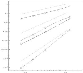
Figure 1: Left: plot of the velocity vector field. Right: convergence plot, errors against mesh size, filled lines $|u_{h}|_{s_{V}}+|z_{h}|_{s_{W}}$, dashed lines $L^{2}$-norm error, dotted lines reference slopes, from top to bottom $\mathcal{O}(h)$, $\mathcal{O}(h^{2})$, $\mathcal{O}(h^{3})$.

In the right plot of Figure 1 we observe optimal convergence rates as predicted by theory (the dual adjoint problem is well-posed, see Bu13 ; CF88 ).

6.2 The elliptic Cauchy problem

Here we consider the problem (5) with $\sigma$ the identity matrix and $c\equiv 0$. We impose the Cauchy data, i.e. both Dirichlet and Neumann data, on boundaries $x=1,\,0<y<1$ and $y=1,\,0<x<1$. We then solve (5) using the method (12) with (14)-(16) and (18) with $k=1$ and $k=2$.

In Figure 2, we present a study of the $L^{2}$-norm error under variation of the stabilisation parameter. The computations are made on one mesh, with $32$ elements per side and the Cauchy problem is solved with $k=1,2$ and different values for $\gamma_{S}$ with $\gamma_{D}=10$ fixed. The level of $10\%$ relative error is indicated by the horizontal dotted line. Observe that the robustness with respect to stabilisation parameters is much better for second order polynomial approximation. Indeed in that case the $10\%$ error level is met for all parameter values $\gamma_{S}\in[2.0E-5,1]$, whereas in the case of piecewise affine approximation one has to take $\gamma_{S}\in[0.003,0.05]$. Similar results for the boundary penalty parameter not reported here showed that the method was even more robust under perturbations of $\gamma_{D}$. In the left plot of Figure 3 we present the contour plot of the interpolated error $i_{V}u-u_{h}$ and in the right, the contour plot of $z_{h}$. In both cases the error is concentrated on the boundary where no boundary conditions are imposed for that particular variable.

In Figure 4 we present the convergence plots for piecewise affine and quadratic approximations. The same stabilisation parameters as in the previous example were used. In both cases we observe the optimal convergence of the stabilisation terms, $\mathcal{O}(h^{k})$, predicted by Lemma 1. For the global $L^{2}$-norm of the error we observe experimental convergence of inverse logarithmic type, as predicted by theory. Note that the main effect of increasing the polynomial order is a decrease in the error constant as expected..

For the local $L^{2}$-norm error, measured in the subdomain $(0.5,1)^{2}$, higher convergence orders, $\mathcal{O}(h^{k})$, were obtained in both cases.

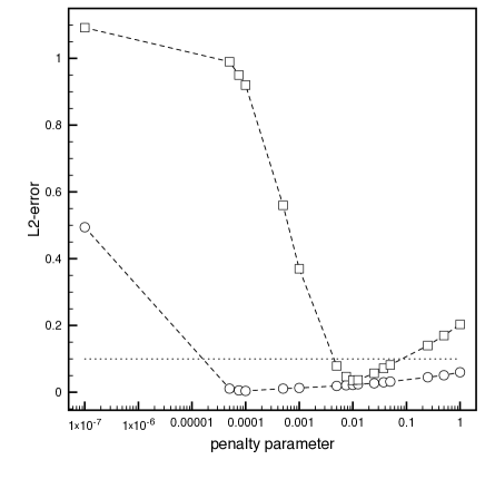
Figure 2: Study of the global $L^{2}$-norm error under variation of the stabilisation parameter, circles: affine elements, squares: quadratic elements

Figure 3: Contour plots of the interpolated error $i_{h}u-u_{h}$ (left plot) and the error in the dual variable $z_{h}$ (right plot).

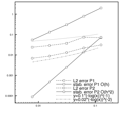
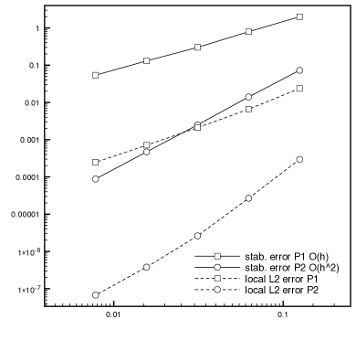
Figure 4: Convergence under mesh refinement, the same slopes for the stabilization semi-norm are represented in both graphics for reference.

The effect of perturbations in data

In this section we will consider some numerical experiments with perturbed data. We consider a perturbation of the form $\delta\psi=\varsigma v_{rand}\psi$ where $v_{rand}$ is a random function defined as a fourth order polynomial on the mesh with random nodal values in $[0,1]$ and $\varsigma>0$ gives the relative strength of the perturbation. We consider the same computations as for unperturbed data. In all figures we report the stabilisation semi-norm $|z_{h}|_{s_{W}}+|u_{h}|_{s_{V}}$ to explore to what extent it can be used as an a posteriori quantity to tune the stabilisation parameter and to detect loss of convergence due to perturbed data.

First we consider the determination of the penalty parameter. First we fix $\gamma_{D}=10$. Then, in Figure 5 we show the results obtained by varying $\gamma_{S}$ when the data is perturbed with $\varsigma=0.01$. We compare the global $L^{2}$-error with the stabilisation semi-norm. For the piecewise affine case we observe that the optimal value of the penalty parameter does not change much. It is taken in the interval $[0.01,0.1]$, which corresponds very well with the minimum of the a posteriori quantity $|z_{h}|_{s_{W}}+|u_{h}|_{s_{V}}$. For piecewise quadratic approximation there is a stronger difference compared to the unperturbed case. The optimal penalty parameter is now taken in the interval $[0.5,5]$. The a posteriori quantity takes its minimum value in the interval $[0.1,0.5]$. From this study we fix the penalty parameter to $\gamma_{S}=0.05$ for piecewise affine approximation and to $\gamma_{S}=1.0$ in the piecewise quadratic case.

Next we study the sensitivity of the error to variations in the strength of the perturbation, for the chosen penalty parameters. The results are given in Figure 6. As expected the global $L^{2}$-error is minimal for the perturbation $\varsigma=0.01$. For smaller perturbations it remains approximately constant, but for perturbations larger than $1\%$ the error growth is linear in $\varsigma$ for all quantities as predicted by theory, assuming the stability condition is satisfied uniformly (see Lemma 3 and Theorem 5.1.)

Finally we study the convergence under mesh refinement when $\varsigma=0.01$. The results are presented in Figure 7. From the theory we expect the reduction of the error to stagnate or even start to grow when $h\lesssim\varsigma$. For the piecewise affine approximation the minimal global $L^{2}$-error is $0.065$ for $h=0.015625$ and it follows that the stagnation takes place for $h\approx\varsigma$ in this case. For $k=2$ the minimal global $L^{2}$-error is $0.047$ for $h=0.03125$, that is one refinement level earlier than for the piecewise affine case. In both cases we observe that the convergence of the stabilisation semi-norm degenerates to worse than first order immediately after the critical mesh-size. The dotted lines without markers immediately below the curve representing the a posteriori quantity are reference curves with slopes $O(h^{1.1})$ for affine elements and $O(h^{1.4})$ for quadratic elements $k=2$. This rate is suboptimal in the latter case, indicating a higher sensibility to perturbations for higher order approximations. It follows that regardless of the smoothness of the (unperturbed) exact solution, high order approximation only pays if perturbations in data are small enough so that they do not dominate before the asymptotic range is reached.

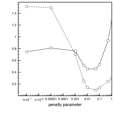
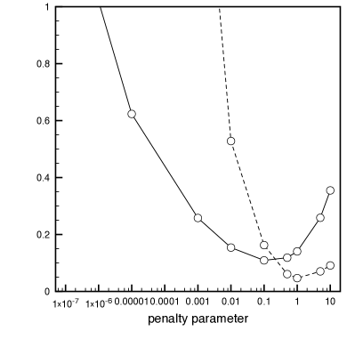
Figure 5: Variation of the global $L^{2}$-error (dashed line) and $|z_{h}|_{s_{W}}+|u_{h}|_{s_{V}}$ (full line) against $\gamma$. Left $k=1$. Right $k=2$.

Figure 6: Variation of the $L^{2}$-error (global dashed line, local dotted line) and $|z_{h}|_{s_{W}}+|u_{h}|_{s_{V}}$ (full line) against $\varsigma$. Left $k=1$. Right $k=2$.

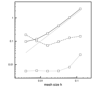
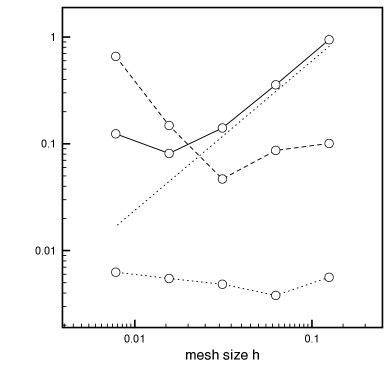
Figure 7: Variation of the $L^{2}$-error (global dashed line, local dotted line) and $|z_{h}|_{s_{W}}+|u_{h}|_{s_{V}}$ (full line, with markers) against $h$. Left $k=1$, reference $O(h^{1.1})$. Right $k=2$, reference $O(h^{1.4})$

6.3 The elliptic Cauchy problem for the convection–diffusion operator

As a last example we consider the Cauchy problem using the noncoercive convection–diffusion operator (56). The stability of the problem depends strongly on where the boundary conditions are imposed in relation to the inflow and outflow boundaries. Strictly speaking this problem is not covered by the theory developed in ARRV09 . Indeed in that work the quantitative unique continuation used the symmetry of the operator. An extension to the convection-diffusion case is likely to be possible, at least in two space dimensions, by combining the results of Ales12 with those of ARRV09 .

To illustrate the dependence of the stability on how boundary data is distributed on inflow and outflow boundaries we propose two configurations. Recalling the left plot of Figure 1 we observe that the flow enters along the boundaries $y=0$, $y=1$ and $x=1$ and exits on the boundary $x=0$. Note that the strongest inflow takes place on $y=0$ and $x=1$, the flow being close to parallel to the boundary in the right half of the segment $y=1$. We propose the two different Cauchy problem configurations:

Case 1.

We impose Dirichlet and Neumann data on the two inflow boundaries $y=0$ and $x=1$.

Case 2.

We impose Dirichlet and Neumann data on the two boundaries $x=0$ and $y=1$ comprising both inflow and outflow parts.

The gradient penalty operator has been weighted with the Péclet number as suggested in Bu13 , to obtain optimal performance in all regimes. In the first case the main part of the inflow boundary is included in $\Gamma_{S}$ whereas in the second case the outflow portion or the inflow portion of every streamline are included in the boundary portion $\Gamma_{S}$ where data are set. This highlights two different difficulties for Cauchy problems for the convection–diffusion operator, in Case 1 the crosswind diffusion must reconstruct missing boundary data whereas in Case 2 we must solve the problem backward along the characteristics, essentially solving a backward heat equation.

In Figure 8, we report the results on the same sequence of unstructured meshes used in the previous examples for piecewise affine approximations and the two problem configurations. In the left plot of Figure 8 we see the convergence behaviour for Case 1, when piecewise affine approximation is used. The global $L^{2}$-norm error clearly reproduces the inverse logarithmic convergence order predicted by the theory for the symmetric case. In the right plot of Figure 8 we present the convergence plot for Case 2 (the dotted lines are the same inverse logarithmic reference curves as in the left plot). In this case we see that the convergence initially is approximately linear, similarly as that of the stabilisation term. For finer meshes however the inverse logarithmic error decay is observed, but with a much smaller constant compared to Case 1. In Case 1 the diffusion is important on all scales, since some characteristics have no data neither on inflow or outflow, whereas in Case 2, data is set either on the inflow or the outflow for all characteristics of the flow and the effects of diffusion are therefore much less important, in particular on coarse scales. Indeed the reduced transport problem in the limit of zero diffusivity, is not ill-posed. As the flow is resolved the effect of the diffusion once again dominates and the inverse logarithmic decay reappears.

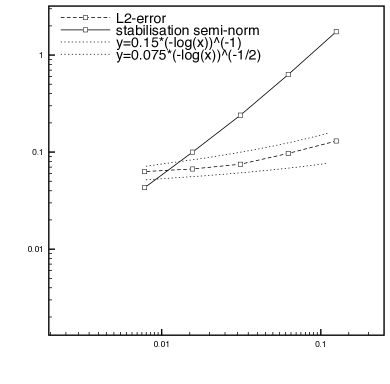
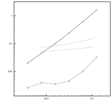
Figure 8: Left: convergence for Case 1, k=1. Right: convergence for Case 2, k=1

7 Conclusion

We have proposed a framework using stabilised finite element methods for the approximation of ill-posed problems that have a conditional stability property. The key element is to reformulate the problem as a pde-constrained minimisation problem that is regularized on the discrete level using tools known from the theory of stabilised FEM. Using the conditional stability error estimates are derived that are optimal with respect to the stability of the problem and the approximation properties of the finite element spaces. The effect of perturbations in data may also be accounted for in the framework and leads to limits on the possibility to improve accuracy by mesh refinement. Some numerical examples were presented illustrating different aspects of the theory.

There are several open problems both from theoretical and computational point of view, some of which we will address in future work. Concerning the stabilisation it is not clear if the primal and adjoint stabilisation operators should be chosen to be the same, or not? Does the adjoint consistent choice of stabilisation $s_{W}$ have any advantages compared to the adjoint stabilisation (19), that gives stronger control of perturbations? Then comes the question of whether or not high order approximation (i.e. polynomials of order higher than one) can be competitive also in the presence of perturbed data? Can the a posteriori error estimate derived in Theorem 4.1 be used to drive adaptive algorithms? Finally, what is a suitable preconditioner for the linear system? We hope that the present work will help to stimulate discussion on the design of numerical methods for ill-posed problems and provide some new ideas on how to make a bridge between the regularization methods traditionally used and (weakly) consistent stabilised finite element methods.

Appendix

We will here give a proof that the inf-sup stability (22) holds also for the stabilisation (18). We do not track the depedence on $\gamma_{D}$ and $\gamma_{S}$.

Proposition 3

Let $A_{h}[(\cdot,\cdot),(\cdot,\cdot)]$ be defined by (13) with $a_{h}(\cdot,\cdot)$, $s_{W}(\cdot,\cdot)$ and $s_{V}(\cdot,\cdot)$ defined by equation (14), (15), (16) and (18) (or (19) for $s_{W}(\cdot,\cdot)$). Then the inf-sup condition (22) is satisfied for the semi-norm (30).

Proof

We must prove that the $L^{2}$-stabilisation of the jump of the Laplacian gives sufficient control for the inf-sup stability of $\mathcal{L}u_{h}$ evaluated elementwise. It is well known BFH06 that for the quasi-interpolation operator defined in each node $x_{i}$ by

$$(I_{os}\Delta u_{h})(x_{i}):=N_{i}^{-1}\sum_{\{K:x_{i}\in K\}}\Delta u_{h}(x_{i})|_{K},$$

$N_{i}:=\mbox{card}\{K:x_{i}\in K\}$ the following discrete interpolation result holds

$$\|h(\Delta u_{h}-I_{os}\Delta u_{h})\|_{h}\leq C_{os}s^{S}_{V}(u_{h},u_{h})^{\frac{1}{2}}$$ (58)

as well as following the stabilities obtained using trace inequalities, inverse inequalities and the $L^{2}$-stability of $I_{os}$,

$$\|h^{\frac{3}{2}}I_{os}\Delta u_{h}\|_{\mathcal{F}}+\|h^{\frac{5}{2}}\partial_{n}I_{os}\Delta u_{h}\|_{\mathcal{F}}+\|hI_{os}\Delta u_{h}\|_{h}+|h^{2}I_{os}\Delta u_{h}|_{s_{X}}\lesssim\|h\Delta u_{h}\|_{h},$$ (59)

where $X=V,W$. First observe that by taking $(v_{h},w_{h})=(u_{h},z_{h})$ we have

$$|u_{h}|_{s_{V}}^{2}+|z_{h}|_{s_{W}}^{2}=A_{h}[(u_{h},z_{h}),(u_{h},z_{h})].$$

Now let $w^{\mathcal{L}}_{h}=h^{2}I_{os}\mathcal{L}u_{h}=h^{2}(I_{os}\Delta u_{h}+cu_{h})$, $v^{\mathcal{L}}_{h}=h^{2}I_{os}\mathcal{L}^{*}z_{h}$. Using (59) it is straightforward to show that

$$\|h^{\frac{3}{2}}I_{os}\mathcal{L}u_{h}\|_{\mathcal{F}}+\|h^{\frac{5}{2}}\partial_{n}I_{os}\mathcal{L}u_{h}\|_{\mathcal{F}}+\|hI_{os}\mathcal{L}u_{h}\|_{h}+|h^{2}I_{os}\mathcal{L}u_{h}|_{s_{X}}\leq\tilde{C}_{os}\|h\mathcal{L}u_{h}\|_{h}.$$ (60)

Now observe that (for a suitably chosen orientation of the normal on interior faces)

$$a_{h}(u_{h},w^{\mathcal{L}}_{h})=\|h\mathcal{L}u_{h}\|^{2}_{h}+(\mathcal{L}u_{h},h^{2}(I_{os}\mathcal{L}u_{h}-\mathcal{L}u_{h}))_{h}+\left<\llbracket\partial_{n}u_{h}\rrbracket,h^{2}I_{os}\mathcal{L}u_{h}\right>_{\mathcal{F}_{I}}\\ +\left<\partial_{n}u_{h},h^{2}I_{os}\mathcal{L}u_{h}\right>_{\Gamma_{N}}+\left<\partial_{n}h^{2}I_{os}\mathcal{L}u_{h},u_{h}\right>_{\Gamma_{D}}\\ \geq\frac{1}{2}\|h\mathcal{L}u_{h}\|^{2}_{h}-2\|h^{2}(I_{os}\mathcal{L}u_{h}-\mathcal{L}u_{h})\|_{h}^{2}-2\tilde{C}_{os}^{-2}s_{V}^{D}(u_{h},u_{h})\\ \geq\frac{1}{2}\|h\mathcal{L}u_{h}\|^{2}_{h}-2C^{2}_{os}s_{V}^{S}(u_{h},u_{h})-2\tilde{C}_{os}^{-2}s_{V}^{D}(u_{h},u_{h})\\ \geq\frac{1}{2}\|h\mathcal{L}u_{h}\|^{2}_{h}-2(C^{2}_{os}+\tilde{C}_{os}^{-2})|u_{h}|_{s_{V}}^{2}$$

and

$$s_{W}(z_{h},w^{\mathcal{L}}_{h})\geq-\tilde{C}_{os}^{-2}|z_{h}|_{s_{W}}^{2}-\frac{1}{4}\|h\mathcal{L}u_{h}\|_{h}^{2}.$$

Similarly

$$a_{h}(v^{\mathcal{L}}_{h},z_{h})\geq\frac{1}{2}\|h\mathcal{L}^{*}z_{h}\|^{2}_{h}-2(C^{2}_{os}+\tilde{C}_{os}^{-2})|z_{h}|_{s_{W}}^{2}$$

and

$$s_{V}(u_{h},v^{\mathcal{L}}_{h})\geq-\tilde{C}_{os}^{-2}|u_{h}|_{s_{V}}^{2}-\frac{1}{4}\|h\mathcal{L}^{*}z_{h}\|_{h}^{2}.$$

It follows that for some $c_{1},c_{2}>0$ there holds

$$|(u_{h},z_{h})|_{\mathcal{L}}^{2}\lesssim A_{h}[(u_{h},z_{h}),(u_{h}+c_{1}w^{\mathcal{L}}_{h},z_{h}+c_{2}v^{\mathcal{L}}_{h})].$$

We conclude by observing that by inverse inequalities and (60) we have the stability

$$|(u_{h}+c_{1}w^{\mathcal{L}}_{h},z_{h}+c_{2}v^{\mathcal{L}}_{h})|_{\mathcal{L}}\lesssim|(u_{h},z_{h})|_{\mathcal{L}}.$$

∎

References

- [1] G. Alessandrini. Strong unique continuation for general elliptic equations in 2D. J. Math. Anal. Appl., 386(2):669–676, 2012.
- [2] G. Alessandrini, L. Rondi, E. Rosset, and S. Vessella. The stability for the Cauchy problem for elliptic equations. Inverse Problems, 25(12):123004, 47, 2009.
- [3] S. Andrieux, T. N. Baranger, and A. Ben Abda. Solving Cauchy problems by minimizing an energy-like functional. Inverse Problems, 22(1):115–133, 2006.
- [4] M. Azaïez, F. Ben Belgacem, and H. El Fekih. On Cauchy’s problem. II. Completion, regularization and approximation. Inverse Problems, 22(4):1307–1336, 2006.
- [5] F. Ben Belgacem. Why is the Cauchy problem severely ill-posed? Inverse Problems, 23(2):823–836, 2007.
- [6] L. Bourgeois. A mixed formulation of quasi-reversibility to solve the Cauchy problem for Laplace’s equation. Inverse Problems, 21(3):1087–1104, 2005.
- [7] L. Bourgeois. Convergence rates for the quasi-reversibility method to solve the Cauchy problem for Laplace’s equation. Inverse Problems, 22(2):413–430, 2006.
- [8] L. Bourgeois and J. Dardé. About stability and regularization of ill-posed elliptic Cauchy problems: the case of Lipschitz domains. Appl. Anal., 89(11):1745–1768, 2010.
- [9] L. Bourgeois and J. Dardé. A duality-based method of quasi-reversibility to solve the Cauchy problem in the presence of noisy data. Inverse Problems, 26(9):095016, 21, 2010.
- [10] E. Burman. Stabilized finite element methods for nonsymmetric, noncoercive, and ill-posed problems. Part I: Elliptic equations. SIAM J. Sci. Comput., 35(6):A2752–A2780, 2013.
- [11] E. Burman. A stabilized nonconforming finite element method for the elliptic Cauchy problem. Math. Comp. to appear, ArXiv e-prints, June 2014.
- [12] E. Burman. Error estimates for stabilized finite element methods applied to ill-posed problems. C. R. Math. Acad. Sci. Paris, 352(7-8):655–659, 2014.
- [13] E. Burman. Stabilized finite element methods for nonsymmetric, noncoercive, and ill-posed problems. Part II: Hyperbolic equations. SIAM J. Sci. Comput., 36(4):A1911–A1936, 2014.
- [14] E. Burman, M. A. Fernández, and P. Hansbo. Continuous interior penalty finite element method for Oseen’s equations. SIAM J. Numer. Anal., 44(3):1248–1274, 2006.
- [15] I. Capuzzo-Dolcetta and S. Finzi Vita. Finite element approximation of some indefinite elliptic problems. Calcolo, 25(4):379–395 (1989), 1988.
- [16] C. Chainais-Hillairet and J. Droniou. Finite-volume schemes for noncoercive elliptic problems with Neumann boundary conditions. IMA J. Numer. Anal., 31(1):61–85, 2011.
- [17] A. Chakib and A. Nachaoui. Convergence analysis for finite element approximation to an inverse Cauchy problem. Inverse Problems, 22(4):1191–1206, 2006.
- [18] S. Christiansen. private communication. 1999.
- [19] B. Cockburn, C. Johnson, C.-W. Shu, and E. Tadmor. Advanced numerical approximation of nonlinear hyperbolic equations, volume 1697 of Lecture Notes in Mathematics. Springer-Verlag, Berlin; Centro Internazionale Matematico Estivo (C.I.M.E.), Florence, 1998. Papers from the C.I.M.E. Summer School held in Cetraro, June 23–28, 1997, Edited by Alfio Quarteroni, Fondazione C.I.M.E.. [C.I.M.E. Foundation].
- [20] J. Dardé, A. Hannukainen, and N. Hyvönen. An -based mixed quasi-reversibility method for solving elliptic Cauchy problems. SIAM J. Numer. Anal., 51(4):2123–2148, 2013.
- [21] R. Eymard, T. Gallouët, and R. Herbin. Error estimate for approximate solutions of a nonlinear convection-diffusion problem. Adv. Differential Equations, 7(4):419–440, 2002.
- [22] R. S. Falk and P. B. Monk. Logarithmic convexity for discrete harmonic functions and the approximation of the Cauchy problem for Poisson’s equation. Math. Comp., 47(175):135–149, 1986.
- [23] J. Hadamard. Sur les problèmes aux derivées partielles et leur signification physique. Bull. Univ. Princeton, 1902.
- [24] H. Han, L. Ling, and T. Takeuchi. An energy regularization for Cauchy problems of Laplace equation in annulus domain. Commun. Comput. Phys., 9(4):878–896, 2011.
- [25] W. Han, J. Huang, K. Kazmi, and Y. Chen. A numerical method for a Cauchy problem for elliptic partial differential equations. Inverse Problems, 23(6):2401–2415, 2007.
- [26] M. V. Klibanov and F. Santosa. A computational quasi-reversibility method for Cauchy problems for Laplace’s equation. SIAM J. Appl. Math., 51(6):1653–1675, 1991.
- [27] R. Lattès and J.-L. Lions. The method of quasi-reversibility. Applications to partial differential equations. Translated from the French edition and edited by Richard Bellman. Modern Analytic and Computational Methods in Science and Mathematics, No. 18. American Elsevier Publishing Co., Inc., New York, 1969.
- [28] H.-J. Reinhardt, H. Han, and D. N. Hào. Stability and regularization of a discrete approximation to the Cauchy problem for Laplace’s equation. SIAM J. Numer. Anal., 36(3):890–905, 1999.
- [29] A. N. Tikhonov and V. Y. Arsenin. Solutions of ill-posed problems. V. H. Winston & Sons, Washington, D.C.: John Wiley & Sons, New York-Toronto, Ont.-London, 1977. Translated from the Russian, Preface by translation editor Fritz John, Scripta Series in Mathematics.
- [30] C. Wang and J. Wang. A Primal-Dual Weak Galerkin Finite Element Method for Second Order Elliptic Equations in Non-Divergence Form. ArXiv e-prints, Oct. 2015.