Distributed Balanced Partitioning via Linear Embedding

Abstract

Balanced partitioning is often a crucial first step in solving large-scale graph optimization problems, e.g., in some cases, a big graph can be chopped into pieces that fit on one machine to be processed independently before stitching the results together, leading to certain suboptimality from the interaction among different pieces. In other cases, links between different parts may show up in the running time and/or network communications cost, hence the desire to have small cut size.

We study a distributed balanced partitioning problem where the goal is to partition the vertices of a given graph into $k$ pieces so as to minimize the total cut size. Our algorithm is composed of a few steps that are easily implementable in distributed computation frameworks, e.g., MapReduce. The algorithm first embeds nodes of the graph onto a line, and then processes nodes in a distributed manner guided by the linear embedding order. We examine various ways to find the first embedding, e.g., via a hierarchical clustering or Hilbert curves. Then we apply four different techniques including local swaps, minimum cuts on the boundaries of partitions, as well as contraction and dynamic programming.

As our empirical study, we compare the above techniques with each other, and also to previous work in distributed graph algorithms, e.g., a label propagation method [UB13], FENNEL [TGRV14] and Spinner [MLS14]. We report our results both on a private map graph and several public social networks, and show that our results beat previous distributed algorithms: e.g., compared to the label propagation algorithm [UB13], we report an improvement of $15$-$25\%$ in the cut value. We also observe that our algorithms allow for scalable distributed implementation for any number of partitions. Finally, we apply our techniques for the Google Maps Driving Directions to minimize the number of multi-shard queries with the goal of saving in CPU usage. During live experiments, we observe an $\approx 40\%$ drop in the number of multi-shard queries when comparing our method with a standard geography-based method.

1 Introduction

Graph partitioning is a crucial first step in developing a tool for mining big graphs or solving large-scale optimization problems. In many applications, the partition sizes have to be balanced or almost balanced so that each part can be handled by a single machine to ensure the speedup of parallel computing over different parts. Such a balanced graph partitioning tool is applicable throughout scientific computation for dealing with distributed computations over massive data sets, and serves as a tradeoff between the local computation and total communication amongst machines. In several applications, a graph serves as a substitute for the computational domain [DFF⁺03]. Each vertex denotes a piece of information and edges denote dependencies between information. Usually, the goal is to partition the vertices where no part is too large, and the number of edges across parts is small. Such a partition implies that most of the work is within a part and only minimal work takes place between parts. In these applications, links between different parts may show up in the running time and/or network communications cost. Thus, a good partitioning minimizes the amount of communication during a distributed computation. In other applications, a big graph can be carefully chopped into parts that fit on one machine to be processed independently before finally stitching the individual results together, leading to certain suboptimality arising from the interaction between different parts. To formally capture these situations, we study a balanced partitioning problem where the goal is to partition the vertices of a given graph into $k$ parts so as to minimize the total cut size.

This is a challenging problem that is computationally hard even for medium-size graphs [AR06] as it captures the graph bisection [GJ79b], hence all attempts at tackling it necessarily relies on heuristics. While the topic of large-scale balanced graph partitioning has attracted significant attention in the literature [DGRW11, DGRW12, TGRV14, UB13], the large body of previous work study large-scale but non-distributed solutions to this problem. Several motivations necessitate the quest for a distributed algorithm for these problems: (i) first of all, huge graphs with hundreds of billions of edges that do not fit in memory are becoming increasingly common [TGRV14, UB13]; (ii) in many distributed graph processing frameworks such as Pregel [MAB⁺10], Apache Giraph [CK10], and PEGASUS [KTF09], we need to partition the graph into different pieces, since the underlying graph does not fit on a single machine, and therefore for the same reason, we need to partition the graph in a distributed manner; (iii) the ability to run a distributed algorithm using a common distributed computing framework such as MapReduce on a distributed computing platform consisting of commodity hardware makes an algorithm much more widely applicable in practice; and (iv) even if the graph fits in memory of a super-computer, implementing some algorithms requires superlinear memory which is not feasible on a single machine. The need for distributed algorithms has been observed by several practical and theoretical research papers [UB13, TGRV14].

For streaming and some distributed optimization models, Stanton [Sta14] has recently shown that achieving formal approximation guarantees is information theoretically impossible, say, for a class of random graphs. Given the hardness of this problem, we explore several distributed heuristic algorithms. Our algorithm is composed of a few logical, simple steps, which can be implemented in various distributed computation frameworks, e.g., MapReduce [DG04].

An application in Google Maps driving directions. As one of the applications of our balanced partitioning algorithm, we study a balanced partitioning problem in the Google Maps Driving Directions. This system computes the optimal driving route for any given source-destination query (pairs of points on Google Maps). In order to answer such pairwise queries in this large-scale graph application, a plausible approach is to obtain a suitable partitioning of the graph beforehand so that each server handles its own section of the graph. In this application, ideally we seek to minimize the number of cross-shard queries, for which the source and destination are not in the same shard, i.e., the total cross-shard traffic is as low as possible, since handling cross-shard queries is much more costly and entails extra communication and coordination across multiple servers. In order to reduce the cross-shard query traffic we want to minimize the cut size between the partitions, with the expectation that less directions will be produced where the source and the destination are in different partitions. Reducing the cut size in practice results in denser regions in the same partition, therefore most queries will be contained within one shard. We confirm this observation with extensive studies using historical query data and live experiments (see Section 6.5 for more details). Conveniently, a linear embedding provides a very simple way of specifying partitions by merely providing two numbers for each shard’s boundaries. Therefore it is straightforward and fast to identify the shard a given query point belongs to. As we will discuss later, our study of linear embedding of graphs while minimizing the cut size is partly motivated by these reasons.

Our Contributions. Our contributions in this paper can be divided into five categories.

1) We introduce a multi-stage distributed optimization framework for balanced partitioning based on first embedding the graph into a line and then optimizing the clusters guided by the order of nodes on the line. This framework is not only suitable for distributed partitioning of a large-scale graph, but also it is directly applicable to balanced partitioning applications like those in Google Maps Driving Directions described above. More specifically, we develop a general technique that first embeds nodes of the graph onto a line, and then post-processes nodes in a distributed manner guided by the order of our linear embedding.

2) As for the initialization stage, we examine several ways to find the first embedding: (i) by naïvely using a random ordering, (ii) for map graphs by the Hilbert-curve embedding, and (iii) for general graphs by applying hierarchical clustering on an edge-weighted graph where the edge weights are based either on the number of common neighbors of the nodes in the graph, or on the inverse of the distance of the corresponding nodes on the map. Whereas the Hilbert-curve embedding and our hierarchical clustering based on node distances may only be applied to maps graphs, the hierarchical clustering based on the number of common neighbors is applicable to all graphs. While all these methods prove useful, to our surprise, the latter (most general) initial embedding technique is the best initialization technique even for maps. We later explain that all these methods have very efficient and scalable distributed implementations. See the discussion in Section 3.3 and Footnote 8 regarding the efficiency of the hierarchical clustering, and the references in Footnote 5 regarding the challenge to construct the similarity metric.

3) As a next step, we apply four methods to postprocess the initial ordering and produce an improved cut. The methods include a metric ordering optimization method, a local improvement method based on random swaps, another based on computing minimum cuts in the boundaries of partitions, and finally a technique based on contracting the min-cut-based clusters, and applying dynamic programming to compute optimal cluster boundaries. Our final algorithm (called Combination) combines the best of our initialization methods, and iterates on the various postprocessing methods until it converges. The resulting algorithm is quite scalable: it runs smoothly on graphs with hundreds of millions of nodes and billions of edges.

4) As our empirical study, we compare the above techniques with each other, and more importantly with previous work. In particular, we compare our results to recent work in (distributed) balanced graph partitioning, including a recent label propagation-based algorithm [UB13], FENNEL [TGRV14], Spinner [MLS14] and METIS [KK98]. We report our results on both a large private map graph, and also on several public social networks studied in previous work [UB13, TGRV14, MLS14, YCLN14].

• First, we show that our distributed algorithm consistently beats the label propagation algorithm by Ugander and Backstrom [UB13] (on LiveJournal) by a reasonable margin for all values of $k$, e.g., for $k=20$, we improve the cut by $25\%$ (from $37\%$ to $27.5\%$ of total edge weight), and for $k=100$, we improve the cut by $15\%$ (from $49\%$ to $41.5\%$). The clustering outputs can be found in [pub15].

• In addition, for $k>2$ partitions, we show that our algorithm beats METIS and FENNEL (on Twitter) by a reasonable factor. For $k=2$, the results that we obtain beats the output of METIS, but it is slightly worse than the result reported by FENNEL.

• For both graphs, our results are consistently superior to that of Spinner [MLS14] with a wide margin.

• We also note that our algorithms allow for scalable distributed implementation for small or large number of partitions. More specifically, changing $k$ from $2$ to tens of thousands does not change the running time significantly.

• As for comparing various initialization methods, we observe that while geographic Hilbert-curve techniques outperform the random ordering, the methods based on the hierarchical clustering using the number of common neighbors as the similarity measure between nodes outperform the geography-based initial embeddings, even for map graphs.

• As for comparing other techniques, we observe the random swap techniques are effective on Twitter, and the min-cut-based or contract and dynamic program techniques are very effective for the map graphs. Overall, we realize that these techniques complement each other, and combining them in a Combination algorithm is the most effective method.

5) As mentioned earlier, we apply our results to the Google Maps Driving Directions application, and deploy two linear-embedding-based algorithms on the World’s Map graph. We first examine the best imbalance factor for our cut-optimization technique, and observe that we can reduce $21\%$ of cross-shard queries by increasing the imbalance factor from $0\%$ to $10\%$. The two methods that we examined via live experiments were (i) a baseline approach based on the Hilbert-curve embedding, and (ii) one method based on applying our cut-optimization post-processing techniques. By running live experiments on the real traffic, we observe the number of multi-shard queries from our cut-optimization techniques is 40$\%$ less compared to the baseline Hilbert embedding technique. This, in turn, results in less CPU usage in response to queries.

Other Related Work. Balanced partitioning is a challenging problem to approximate within a constant factor [GH88, AR06, FK02], or to approximate within any factor in several distributed or steaming models [Sta14]. As for heuristic algorithms for this problem in the distributed or streaming models, a number of recent papers have been written about this topic [SK12, UB13, TGRV14]. Our algorithms are different from the ones studied in these papers. The most similar related work are the label propagation-based methods of Ugander and Backstrom [UB13] and Martella et al. (Spinner) [MLS14] which develop a scalable distributed algorithm for balanced partitioning. Our random swap technique is similar in spirit to the label propagation algorithm studied by [UB13], however, we also examine three other methods as a postprocessing stage and find out that these methods work well in combination. Moreover, [UB13] studied two different methods for their initialization, a random initialization, and a geographic initialization. We also examine random ordering, and a Hilbert-curve ordering which is similar to the geographic initialization by [UB13], however we examine two other initialization techniques and observe that even for map-based geographic graphs, the initialization methods based on hierarchical clustering outperform the geography-based initial ordering. Overall, we compare our algorithm directly on a LiveJournal public graph (the only public graph reported in [UB13]), and improve the cut values achieved in [UB13, MLS14] by a large margin for all values of $k$. In addition, algorithms developed in [SK12, TGRV14] are suitable for the streaming model, but one can implement variants of those algorithms in a distributed manner. We also compare our algorithm directly to the numbers reported on the large-scale Twitter graph by FENNEL [TGRV14], and show that our algorithm compares favorably with the FENNEL output, hence indirectly comparing against [SK12] because of the comparison provided in [TGRV14].

Motivated by a variety of big data applications, distributed clustering has attracted significant attention over the literature, both for applications with no strict size constraints on the clusters [EIM11, BMV⁺12, BEL13], or with explicit or implicit size constraints [BBLM14]. A main difference between such balanced clustering problems and the balanced graph partitioning problems considered here is that in the graph partitioning problems a main objective function is to minimize the cut function, but in those clustering problems, the main goal is minimize the maximum or average distance of nodes to the center of those clusters.

2 Preliminaries

For an integer $n$, we define $[n]=\{1,2,\dots,n\}$. We also slightly abuse the notation and, for a function $f:A\mapsto\mathbb{R}$, define $f(A^{\prime})=\sum_{a\in A^{\prime}}f(a)$ if $A^{\prime}\subseteq A$. For a function $f:S\mapsto T$, we let $f^{-1}(t)$ for $t\in T$ denote the set of elements in $S$ mapped to $t$ via $f$. For a permutation $\pi$, let $\pi_{i}$ denote, for $i\in[n]$, the element in position $i$ of $\pi$. Moreover, let $\pi(i\rightarrow j)=\{\pi_{i},\pi_{i+1},\dots,\pi_{j}\}$ for $i\in[n],j\in[n]\cup\{0\}$. Note that, in particular, $\pi(i\rightarrow j)=\emptyset$ if $j<i$.

2.1 Problem definition

Given is a graph $G(V,E)$ of $n$ vertices with edge lengths and node weights, as well as an integer $k$, and a real number $\alpha\geq 0$. Let us denote the edge lengths by $d:E\mapsto\mathbb{R}$, and the vertex weights by $w:V\mapsto\mathbb{R}$. A partition of vertices of $G$ into $k$ parts $\{V_{i}:i\in[k]\}$ is said to be $\alpha$-balanced if and only if

$$(1-\alpha)\frac{w(V)}{k}\leq w(V_{i})\leq(1+\alpha)\frac{w(V)}{k}.$$

In particular, a zero-balanced (or fully balanced) partition is one where all partitions have the same weight. The cut length of the partition is the total sum of all edges whose endpoints fall in different parts:

$$\sum_{i}\sum_{j<i}\sum_{u\in V_{i}}\sum_{v\in V_{j}:(u,v)\in E(G)}w(u,v).$$

Our goal is to find an $\alpha$-balanced partition whose cut size is (approximately) minimized.

The problem is NP-hard as the case of $\alpha=0,k=2$ is equivalent to the minimum bisection problem [GJ79a]. For arbitrary $k$, we get the minimum balanced $k$-cut problem, that is known to be inapproximable within any finite factor [AR06]; the best known approximation factor for it is $O(\log^{1.5}n)$ (if $\alpha>0$ is constant).

2.2 Our algorithm

Our algorithm consists of three main parts:

1. We first find a suitable mapping of the vertices to a line. This gives us an ordering of the vertices that presumably places (most) neighbors close to each other, therefore somewhat reduces the minimum-cut partitioning problem to an almost local optimization one.

2. We next attempt to improve the ordering mainly by swapping vertices in a semilocal manner. These moves are done so as to improve certain metrics (perhaps, the cut size of a fully balanced partition).

3. Finally, we use local postprocessing optimization in the “split windows” (i.e., a small interval around the equal-size partitions cut points taking into account permissible imbalance) to improve the partition’s cut size.

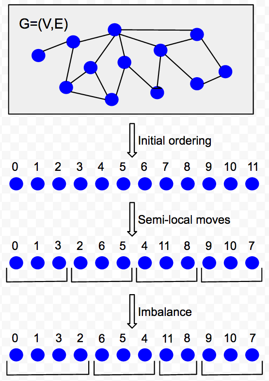
Figure 1: A natural flow for our algorithm. The vertices of $G$ are first embedded on a line, then the embedding is improved via swaps, and finally imbalanced clusters are created according to the ordering of vertices. As we explain later on, iterating on these steps yields better results.

Note that one implementation may use only some of the above, and clearly any implementation will pick one method to perform each task above and mix them to get a final almost balanced partition. Indeed, we report some of our results (specially those in comparison to the previous work) based on Combination, which uses AffCommNeigh to get the initial ordering and then iteratively applies techniques from the second and third stages above (e.g., Metric, Swap, MinCut) until the result converges. (The convergence in our experiments happens in two/three rounds.)

Algorithm 1 $\texttt{Combination}(G,k,\alpha)$

Input: Graph $G$, number of parts $k$, imbalance param. $\alpha$
Output: A partition of $V(G)$ into $k$ parts

1:  for all $(u,v)\in E(G)$ do

2:     $w(u,v)\leftarrow$ number of common neighbors of $u,v$

3:  $\pi\leftarrow\texttt{AffinityOrdering}(G,w)$

4:  for $i=0$ to $k$ do

5:     $q(i)\leftarrow\lfloor\frac{in}{k}\rfloor$ {fully balanced split points}

6:  repeat

7:     $(\pi^{\prime},q^{\prime})\leftarrow(\pi,q)$

8:     Use any (semilocal or imbalance-inducing) postprocessing technique on $(G,\pi^{\prime},q^{\prime})$ to obtain $(\pi,q)$

9:  until $\pi=\pi^{\prime}$ and $q=q^{\prime}$

10:  for all $i\in[k]$ do

11:     $V_{i}\leftarrow\pi(q(i)+1\rightarrow q(i+1))$

12:  return  $\{V_{1},V_{2},\dots,V_{k}\}$

3 Initial mapping to line

3.1 Random mapping

The easiest method to produce an ordering for the vertices is to randomly permute them. Though very fast, this method does not seem to lead to much progress towards our goal of finding good cuts. In particular, if we then turn this ordering into a partition by cutting contiguous pieces of equal size, we end up with a random partitiong of the input (into equal parts) which is almost surely a bad cut: a standard probablistic argument shows that the cut has expected ratio $1-\frac{1}{k}$. Nevertheless, the next stage of the algorithm (i.e., the semilocal optimization by swapping) can generate a relatively good ordering with this naïve starting point.

3.2 Hilbert curve mapping

For certain graphs, geographic/geometric information is available for each vertex. It is fairly easy, then, to construct an ordering using a space-filling curve—prime examples are Peano, Morton and Hilbert curves, but we focus on the latter in this work. These methods are known to capture proximity well: nodes that are close in the space are expected to be placed nearby on the line.

There has been extensive study of the applicability of these methods in solving largescale optimization problems in parallel; see, e.g., [SS00, MJFS01].

Not only can this algorithm be used on its own without any cut guarantees, but it can also be employed to break a big instance down into smaller ones that we can afford to run more intensive computations on. Both applications were known previously.

The previous works do not offer any theoretical guarantees on the quality of the cut generated from Hilbert curves. However, certain assumptions on the distributions of edge lengths and node positions let us bound the resulting cut ratio, and show that it is significantly less than the result of random ordering [GL96, NRS02, FTW00]. This is observed in our experiments, too.

3.3 Affinity-based mapping

One drawback of the Hilbert curve cover (even when coordinates are available) is that it ignores the actual edges in the graph. For an illustration, consider using the Hilbert curve to map certain points in an archipalego (or just a small number of islands or peninsulas). The Hilbert curve, unaware of the connectivities, traverses the vertices in a semirandom order, therefore, it may jump from island to island without covering the entire island first.

To address this issue, we use an agglomerative hierarchical clustering method, usually called average-linkage clustering. We call the method “affinity clustering” since it takes into account the affinity of vertices. Informally, every node starts in a singleton cluster of its own, and then in several stages we group vertices that are closely connected, hence building a tree of these connections. More precisely, at every stage, each node turns on the connection to its closest neighbor, after which the connected components form clusters. The similarities used in the next level between constructed clusters are computed via some function of the similarities between the elements forming the clusters; in particular, we take the average function for this purpose.

The final ordering is produced by sorting the vertex labels produced as follows. Let the label for each vertex be the concatenation of vertex ID strings from the root to the corresponding leaf. Sorting the constructed labels places the vertices under each branch in a contiguous piece on the line. The same guarantee holds recursively, hence the (edge) proximity is preserved well. A pseudocode for this procedure is given in Algorithm 2: Line 15 uses notation $a\#b$ to denote the concatenation of labels for $a$ and $b$. Notice that this pseudocode explains a sequential algorithm, however, the procedure can be efficiently implemented in a few rounds of MapReduce. In fact, our algorithm is very similar to [RMCS13] but uses Distributed Hash Tables as explained in [KLM⁺14].

Algorithm 2 $\texttt{AffinityOrdering}(G,w)$

Input: Graph $G$, (partial) similarity function $w$
Output: A permutation of vertices

1:  $\mathcal{C}^{0}$ $\leftarrow$$\{\{v\}|v\in V(G)\}$

2:  for $v\in V(G)$ do

3:     $\ell(v)\leftarrow v$

4:  $i\leftarrow 0$

5:  repeat

6:     for $s\in\mathcal{C}^{i}$ do

7:        $\displaystyle p(s)\leftarrow\arg\max_{t\in C^{i}}w(s,t)$

8:     $\mathcal{C}^{i+1}\leftarrow\emptyset$

9:     for $t\in\{p(s)|s\in\mathcal{C}^{i}\}$ do

10:        $S\leftarrow p^{-1}(t)$

11:        $S^{\prime}\leftarrow\bigcup_{s\in S}s$

12:        $\displaystyle\mathcal{C}^{i+1}\leftarrow\mathcal{C}^{i+1}\cup S^{\prime}$

13:        $\displaystyle r\leftarrow\arg\min_{r^{\prime}\in S^{\prime}}s$

14:        for $s^{\prime}\in S^{\prime}$ do

15:           $\ell(s^{\prime})\leftarrow r\#\ell(s^{\prime})$

16:     $i\leftarrow i+1$

17:  until $|\mathcal{C}^{i}|=|\mathcal{C}^{i-1}|$

18:  $\pi\leftarrow$ permutation of vertices sorted according to $\ell$

19:  return  $\pi$

Intuitively, we expect vertices connected in lower levels (farther from the root) to be closer than those connected in later stages. (See Figure 2 for illustration.) In particular, we observed that a graph with several connected components gives an advantage to affinity tree ordering over the ordering produced by Hilbert curve.

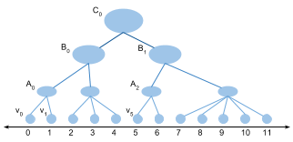
Figure 2: Illustration of Affinity tree ordering. The nodes at the bottom row correspond to the vertices of the graph, and the nodes at the higher levels are formed by merging nodes from lower levels. The vertices are finally sorted in the picture according to their labels. For instance, the label for $v_{0}$ is $C_{0}\#B_{0}\#A_{0}\#v_{0}$ whereas $v_{5}$ is labeled $C_{0}\#B_{1}\#A_{2}\#v_{5}$.

For this approach to work, we require meaningful distances/similarities between vertices of the graph. Conveniently it does not matter whether we have access to distances or similarity values. However, though theoretically possible to run the affinity clustering algorithm on an unweighted graph with distances $1$ and $\infty$ for edges and non-edges respectively, this leads to a lot of arbitrary tie-breaks that makes the result irrelevant.

Fortunately, there are standard ways to impose a metric on an unweighted graph: e.g., common neighbors ratio or personalized page rank. We focus on the former metric and compute for every pair of neighbors the ratio of the number of their common neighbors over the total number of their distinct neighbors. Computing the number of common neighbors can be implemented using standard techniques in MapReduce, however, one can use sampling when dealing with high-degree vertices to improve the running time and memory footprint (leading to an approximate result).

4 Improve ordering using semilocal moves

Given an initial ordering of vertices for example by AffinityOrdering, we can further improve the cut size by applying semilocal moves. The motivation here is that these simple techniques provide us with highly parallelizable algorithms that can be iteratively applied (e.g., by a MapReduce pipeline) so the result converges to high-quality partitions. In the following we discuss two such approaches.

4.1 Minimum Linear Arrangement

Minimum Linear Arrangement (MinLA) is a well studied NP-hard optimization problem [GJ79b]. Given an undirected graph $G=(V,E)$ (with edge weights $w_{uv}$) we seek a one-to-one function $\phi:V\rightarrow\{0,1,\dots,n-1\}$ that minimizes

$$\sum_{(u,v)\in E}|\phi(v)-\phi(u)|w_{uv}.$$ (1)

Optimizing the sum above results in a linear ordering of vertices along a line such that neighbor nodes are nearby each other. The end result is that dense regions of the graph will be isolated into clusters and therefore makes it easier to identify cut boundaries on the line.

We have implemented a very simple distributed algorithm (in MapReduce) that directly optimizes MinLA. The algorithm simply iterates on the following MapReduce phases until it converges (or runs up to a specified number of steps):

• MR Phase 1: Each node computes its optimal rank as the weighted median of its neighbors and outputs its new rank.

• MR Phase 2: Assigns final ranks to each node (i.e., handles duplicate resolution, for example, by simple ID-based ordering).

Note that since Phase 1 is done in parallel for each node and independently of other moves, there will be side effects, hence it is an optimistic algorithm with the hope that it will converge to a stable state after few rounds. Our experimental results show that in practice this algorithm indeed converges for all the graph types that we tried, although the number of rounds depends on the underlying graph.

4.2 Rank Swap

Given an existing linear ordering of vertices in a graph we can further improve the cut size (of the fully balanced partition based on it) via semilocal swaps. Note that unlike MinLA heuristic discussed in Section 4.1, this process depends on the prechosen cut boundaries, i.e., the number of final partitions $k$. Notice that one expects that the semilocal swap operations will be effective once a good initial ordering provided by either the Affinity-based mapping and/or MinLA. Indeed our experimental results show that this procedure is extremely effective and produces cut sizes better than the competition on some public social graphs we tried.

RankSwap can be implemented in a straightforward way on a distributed (for example, MapReduce) framework as outlined by Algorithm 3.

Algorithm 3 $\texttt{RankSwap}(G,k,r)$

Input: Graph $G$, number of partitions $k$, number of intervals per partition $r$
Output: A partition of $V(G)$ into $k$ parts

Controller:

1:      Pair nearby partitions

2:      Split each partition into $r$ intervals $I_{0},\dots,I_{r-1}$ and randomly pair intervals between paired partitionsMap $\langle I_{i};I_{j}\rangle$:

3:  repeat

4:     Pick node pair $u\in I_{i}$, $v\in I_{j}$ with the best cut improvement

5:     Swap $u$ and $v$

6:  until no pair improves the cut

7:  for all $u\in I_{i}\cup I_{j}$ do

8:     Emit $\langle u;r_{u}\rangle$. {$r_{u}$ is the new rank of $u$} Reduce $\langle u;r_{u}\rangle$:

9:      Emit $\langle u;r_{u}\rangle$. {Identity Reducer}

Subdividing each partition into intervals is important, especially for small number of partitions $k$, to achieve parallelism, and allowing possibly more time- and memory-consuming swap operations. Pairing the intervals between two partitions can be done in various ways. One simple example is random pairing. Our experiments showed that this is almost as effective as more complicated ones, hence we do not discuss the other methods in detail here.

The swap operation between two intervals (handled by each Mapper task) can be done in various ways. (The version described in Algorithm 3 is Method 3 below.)

Each approach below starts with computing the cut size reduction as a result of moving a node from one interval to the other. Once these values are computed for each node in the two intervals the following are the alternatives we tried (from the simplest to more complicated):

• Method 1: Sort the nodes in each interval in descending order by their cut size reduction. Then simply do a pairwise swap between entries at $i$th place in each interval provided that the swap results in a combined reduction. This method is very simple and fast, however, it may have side effects within the interval (and also outside) since it does not account for those.

• Method 2: This is a modified version of Method 1 with the addition that after each swap is performed we also update the cut reduction values of other nodes. This method does only one pass from top to bottom and stops when there is no further improvement.

• Method 3: In this method we iterate on Method 2 until we converge to a stable state. In this way we reach a local optimum between two intervals. The other improvement is that instead of pairing entries at $ith$ position we find the best pair in the second interval and swap with that. This is because the top entries in each interval can be neighbors of each other and therefore they may not be the best pair to swap.

Our extensive studies with these methods confirmed that Method 3 gives the best results in terms of quality at the expense of an acceptable additional cost. It runs fast in practice due to the relatively small sizes of the intervals because of the parallelism we achieve. We can also afford an additional cost in the swap method because each interval pair is handled by a separate Mapper task.

5 Imbalance-inducing postprocessing

We have now an ordering of the vertices that presumably places similar vertices close to each other. Instead of cutting the sequence at equidistance positions to obtain a fully balanced partitioning, we describe in this section several postprocessing techniques that allow us to take advantage of the permissible imbalance and produce better cuts.

First we sketch how the problem can be solved optimally if the number of vertices is not too large. This approach is based on dynamic programming and requires the entire graph to live in memory, which is a barrier for using this technique even if the running time were almost linear. However, this algorithm is still usable with the caveat that one first needs to group together blocks of contiguous vertices and contract them into supernodes, such that the graph of supernodes fits in memory and is small enough for the algorithm to handle. The fact that nearby vertices are similar to each other implies that this sort of contraction should not hurt the subsequent optimization significantly. Indeed trying two different block sizes (resulting in $1000$ and $5000$ blocks) produced similar cuts.

The other two approaches work on the concept of “windows” and perform only local optimizations within each. Let $\pi$ denote the permutation of vertices at the start of the local optimization, and let $\pi_{i}$ be the $i$-th vertex in the permutation for $1\leq i\leq n$. Given that we want to get $k$ parts of (almost) the same size, we consider the ideal split points $q_{j}=\lfloor\frac{jn}{k}\rfloor$ for $1\leq j<k$. Though there are only $k-1$ real split points, we define two dummy split points at either end to make the notation cleaner: $q_{0}=0$ and $q_{k}=n$. Then, the ideal partitions, in terms of size, will be formed of $\pi(q_{j}+1\rightarrow q_{j+1})$ for different $0\leq j<k$. Given a permissible imbalance $\alpha>0$, a window is defined around each (real) split point allowing for $\alpha/2$ imbalance on either side. More precisely, $W_{j}=\pi(\pi_{q_{j}-\alpha^{\prime}}\rightarrow\pi_{q_{j}+\alpha^{\prime}})$ for $\alpha^{\prime}=\lceil\frac{\alpha n}{2k}\rceil$. Essentially we are free to shift the boundaries of partitions within each window without violating the balance requirements. We propose two methods to take advantage of this opportunity. One finds the optimal boundaries within windows, while the other also permutes the vertices in each window arbitrarily to find a better solution.

5.1 Dynamic program to optimize cuts

The partitioning problem becomes more tractable if we fix an ordering $\pi$ of vertices and insist on each partition consisting of consecutive vertices (perhaps, with wrap-around). Let us for now assume that no wrap-around is permissible; i.e., each part corresponds to a contiguous subset of vertices on $\pi$.

In the dynamic programming (DP) framework, instead of solving the given instance, we solve several instances (all based on the input and closely related to one another), and do so in a carefully chosen sequence such that the instances already solved make it easier to quickly solve newer instances, culminating in the solution to the real instance.

Let $A_{i,j,q}$ for $1\leq i,j\leq n,1\leq q\leq k,j\geq i-1$ denote the smallest cut size achievable for the subgraph induced by vertices $\pi(i\rightarrow j)$ if exactly $q$ partitions thereof are desired. Once all these entries are computed, $A_{1,n,k}$ yields the solution to the original problem. As is customary in dynamic programs, we only discuss how to find the “cost”—here, the cut size—of the optimal solution; finding the actual solution—here, the partition—can be achieved in a straight-forward manner by adding certain information to the DP table.

We fill in the table $A_{i,j,q}$ in the order of increasing $q$. For the case of $q=1$, we clearly have $A_{i,j,q}=0$ if and only if

$$w(\pi(i\rightarrow j))\leq(1+\alpha)\frac{w(V)}{k},$$

i.e., vertices $\pi(i\rightarrow j)$ can be placed in one part without violating the balanced property. Otherwise, it is defined as infinity.

We use a recurisve formula to compute $A_{i,j,q}$ for $q>1$. The formula depends on $A_{i^{\prime},j^{\prime},q^{\prime}}$ entries where $q^{\prime}<q$, hence these entries have all been already computed. Let us introduce some notation before presenting the recurrence. We define $C(i,j,k)$ as the total length of edges going from $\pi(i\rightarrow j)$ to $\pi(j+1\rightarrow k)$. We now present the recursive formula for computing $A_{i,j,q}$ as

$$A_{i,j,q} =\min_{i-1\leq k\leq j}\left[A_{i,k,1}+A_{k+1,j,q-1}+C(i,k,j)\right].$$ (2)

Notice that the first term in the minimization is only used to signify whether $\pi(i\rightarrow k)$ is a valid part in the intended $\alpha$-balanced partition: its value is either zero or infinity.

Lemma 1.

Equation (2) is a valid recursion for $A_{i,j,q}$, which coupled with the initialization step given above yields a sound computation for all entries in the DP table.

Proof.

The argument proceeds by mathematical induction. The initialization step is clearly sound as it is simply verifying feasiblity of single parts.

For the inductive part, it suffices to show that the best solution with a part $\pi(i\rightarrow k)$ has a cut size $A_{i,k,1}+A_{k+1,j,q-1}+C(i,k,j)$. Then, the first term in (2) accounts for the case when we use one empty part (i.e., we partition $\pi(i\rightarrow j)$ using only $q-1$ parts) and the minimization considers the cases when the first part consists of $\pi(i\rightarrow k)$. To see the cost of thelatter is as in (2), notice that any cut edge in the partition of $\pi(i\rightarrow j)$ is either completely inside $\pi(i\rightarrow k)$ (i.e., not contributing to the cut size), inside $\pi(k+1\rightarrow j)$ (which is accounted for in $A_{k+1,j,q-1}$ or connects $\pi(i\rightarrow k)$ to $\pi(k+1\rightarrow j)$ (in which case is taken into account by $C(i,k,j)$). ∎

The above procedure can be implemented to run in time $O(n^{3}k)$ and consume space $O(n^{2}k)$. Next we show how to improve this further. The key idea is to avoid computing $A_{i,j,q}$ for all values $1\leq q\leq k$. Rather we focus on a limited subset of such $q$’s of size $O(\log k)$.

We start by rewriting the recurrence as

$$A_{i,j,q} =\min_{i-1\leq k<j}\left[A_{i,k,\lfloor\frac{q}{2}\rfloor}+A_{k+1,j,\lceil\frac{q}{2}\rceil}+C(i,k,j)\right].$$ (3)

Then, computing the desired value $A_{1,n,k}$ only requires the computation of $A_{i,j,q}$ where $q$ is either $\lfloor\frac{k}{2^{l}}\rfloor$ or $\lceil\frac{k}{2^{l}}\rceil$ for some $l\geq 0$. This reduces the running time to $O(n^{3}\log k)$, and a bottom-up DP computation needs no more than three different values for $q$, hence the memory requirement is $O(n^{2})$.

5.2 Scalable linear boundary optimization

Recall the notion of “windows” defined at the beginning of Section 5. We now focus on a window $W=W_{j}$. This is small enough so that all information on the vertices in the window (including all their edges ) fit in memory (of one Mapper or Reducer). The linear optimization postprocessing finds a new split point in each window, so that the total weight of edges crossing it is minimized.

Let $B$ and $A$ denote the set of vertices appearing before and after $W$, respectively, in the ordering $\pi$. The edges going from $B$ to $A$ are irrelevant to the local optimization since those edges are necessarily cut no matter what split point we choose. The other edges have at least one endpoint in $W$. Then, there is a simple algorithm of running time $O(|V_{W}|\cdot|E_{W}|)$ to find the best split point in $W$ where $V_{W}$ and $E_{W}$ denote the set of vertices and edges, respectively, corresponding to $W$: look at each candidate split point and go over all relevant edges to determine the weight of the associated cut.

This can be done more efficiently to run in time $O(|V_{W}|+|E_{W}|)$, too. Let $s_{v}$ for $v\in W$ be the cut value (ignoring the effect of the edges between $B$ and $A$). We scan the candidate split points from left to right, and compute $s_{v}-s_{0}$ where $s_{0}=s_{\pi_{q_{j}-\alpha^{\prime}}}$ (i.e., the cut value for the first split point in $W$). For each vertex $v$ following $u$, start with $s_{u}-s_{0}$, remove the edges between $v$ and the vertices to its left (these already showed up in the cut value) and add up the edges between $u$ and the vertices to its right; this gives the cut value $s_{v}-s_{0}$.

Since the windows are relatively small compared to the entire graph, and their corresponding subproblems can be solved independently, there is a very efficient MapReduce implementation for window-based postprocessing methods.

5.3 Scalable minimum-cut optimization

Once again we focus on a window $W=W_{j}$, and denote by $B$ and $A$ the set of vertices belonging to previous and following vertices. Recall that the linear optimization of the previous section finds the best split point in the window while respecting the ordering of the vertices given in the permutation in $\pi$. The minimum-cut optimization, though, finds the best way to partition $W$ into two pieces $W_{L}$ and $W_{R}$ so that the total weight of edges going from $B\cup W_{L}$ to $A\cup W_{R}$ is minimized.

(a) The ordering of vertices on the line prior to MinCut procedure for an instance with $k$ where the three windows are marked. The edges are not shown.

(b) Minimum cut instance for window $W_{2}$. The diagram only shows edges with one endpoint in the window (and excludes any edges coming from beyond the neighboring windows since those are not affected by the choice of the cut). The source node, to which all edges going to the left are attached, and the sink node, to which all edges going to the right are attached, are not shown.

(c) The solution from LinOpt, which respects the ordering within the window and only optimizes for the split point. Solid and empty nodes are the two sides of the cut. The value of the cut is $4$.

(d) The solution from MinCut, which tampers with the ordering within the window. Solid and empty nodes are the two sides of the cut.The value of the cut is $1$.

Figure 3: Illustration of MinCut postprocessing.

6 Empirical studies

First we describe the different datasets that we use in our experiments.

Next we compare our results to previous work, and we finally compare our different methods to each other: i.e., we demonstrate through experiments how much value each ingredient of the algorithm adds to the solution.

6.1 Datasets

We present our results on three datasets: World-roads, Twitter and LiveJournal (as well as publish our output on Friendster). As the names suggest, the first one is a geographic dataset while the last three are social graphs. All are big graphs, representatives of maps and social networks, and we test the quality and scalability of our algorithm on them.

World-roads

A subset of the entire world road network with hundreds of millions of vertices and over a billion edges. (Due to near-planarity, the averagre degree is small.) Edges do not have weights, but vertices have longitude/latitude information. Our algorithms run smoothly on this graph in reasonable time using a small number of machines, demonstrating their scalability.

Twitter

The public graph of tweets, with about 41 million vertices (twitter accounts) and 2.4 billion (directed) edges (denoting followership) [KLPM10]. This graph is unweighted, too. We run all our algorithms on the undirected underlying graph.

LiveJournal

The undirected version of this public social graph (snapshot from 2006) has $4.8$ million vertices and $42.9$ million edges [UB13].

Friendster

The undirected version of this public social graph (snapshot from 2006) has $65.6$ million vertices and $1.8$ billion edges.

6.2 Comparison of different Techniques

6.2.1 Initial ordering

We have four methods to obtain an initial ordering for the geographic graphs and two for non-geographic graphs. Here we compare these methods to each other based on the value of the cut obtained by chopping the resulting order into equal contiguous pieces. In order to make this meaningful, we report all the cut sizes as the fraction of cut edges to the total number of edges in the graph.

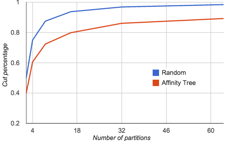
Figure 4: Comparison of the (fully balanced) cut size for RandInit and AffCommNeigh on Twitter.

Figure 4 compares the results of two methods: RandInit produces a random permutation of the vertices, hence, as we observed prevously, gets a cut size of approximately $1-\frac{1}{k}$; AffCommNeigh (using the AffinityOrdering with the similarity oracle based on the number of common neighbors) clearly produces better solutions with improvements ranging from 20% to 10% (more improvement for smaller number of parts). The AffCommNeigh tree in this case was pretty shallow (much lower than the theoretical $\log n$ upper bound) with only four levels. Whenever we report numbers for different number of partitions in one chart, $k=2,4,8,16,32,64$ are used for experiments.

Figure 5 compares the results of three methods, each producing a cut of size at most $3\%$ and significantly improving upon the $1-\frac{1}{k}$ result of RandInit: Compared to Hilbert, the two other methods AffInvDist (using the inverse of geographic distance as the similarity oracle) and AffCommNeigh, respectively, obtain $90\%$ to $50\%$ and $95\%$ to $70\%$ improvement; once again the easier instances are those with smaller $k$. The corresponding trees, with 13 and 11 levels, respectively, are not as shallow as the one for Twitter. The quality of the cuts correlates with the runtime complexity of the algorithms: RandInit (fastest, but worst), Hilbert, AffInvDist, and AffCommNeigh (best, but slowest). Note that although the implementation of Hilbert seems more complicated, it is significantly faster in practice.

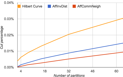
Figure 5: Comparison of the (fully balanced) cut size for Hilbert, AffInvDist and AffCommNeigh on World-roads.

For the following experiments, we focus on AffCommNeigh since it consistently produces better results for different values of $k$ as well as both for Twitter and World-roads . Specially in diagram legends, this initialization step may be abbreviated as Aff.

6.2.2 Improvements and imbalance

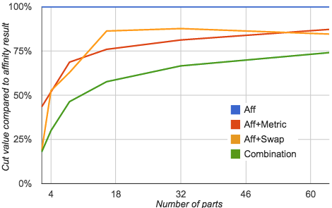
Figure 6: Comparison of the (fully balanced) cut size for three semilocal operations on Twitter. The results are compared to AffCommNeigh, set as 100%.

The performance of the semilocal improvement methods, Aff+Metric and Aff+Swap, as well as our main algorithm, Combination, on Twitter is reported in Figure 6. The diagram shows the percentage of improvement of each over the baseline AffCommNeigh for different values of $k=2,4,\dots,32,64$. Except for $k=16,32$, Aff+Swap outperforms Aff+Metric; their performance varies from $7\%$ to $75\%$, with best performance for smaller $k$. Combining the two methods with the imbalance-inducing techniques to get Combination yields results significantly better than every single ingredient, with the relative improvement sometimes as large as 50%. The final results have very little imbalance, and indeed cuts of comparable quality can be obtained without any imbalance.

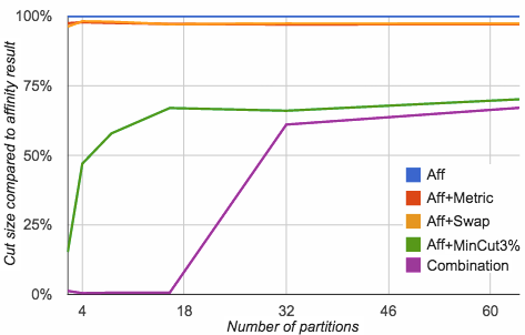
Figure 7: Cut value obtained by semilocal optimization methods on World-roads as compared to their baseline, AffCommNeigh.

Figure 7 also sets the results of various postprocessing methods against one another and depicts their improvements compared to the baseline of AffCommNeigh when run on World-roads. The first two consists of semilocal optimization methods, Aff+Metric and Aff+Swap, which also appeared in the discussion for Twitter. These do not yield significant improvement over their AffCommNeigh starting point: the results compared to the starting point (baseline) ranges from 95% to 98%. The other two algorithms use imbalance-inducing ideas, and yield significantly better results. Our main algorithm, which we call Combination, clearly outperforms all the others specially for small values of $k$.

All the experiments assume $3\%$ imbalance in partition sizes—each partition may have size within range $(1\pm 0.03)\frac{n}{k}$. However, only Aff+MinCut and Combination use this to improve the quality of the partition.

6.2.3 Convergence analysis

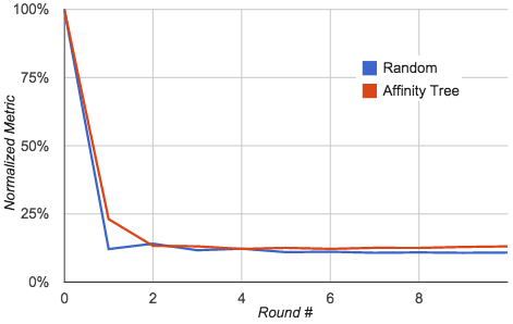
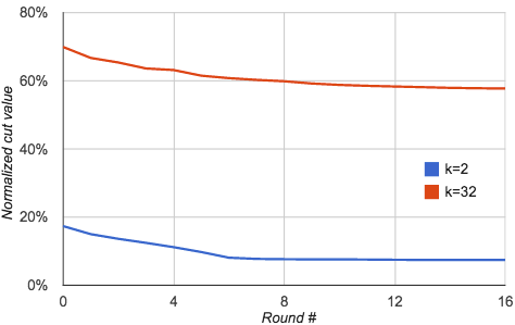
Figure 8: Convergence rate of Aff+Metric (top) and Aff+Swap (bottom) on Twitter.

Next we consider the convergence rate of the two semilocal improvement methods on two graphs. For Twitter, the rate of convergence for metric optimization is the same whether we start with AffCommNeigh or RandInit. (See Figure 8.) The convergence happens essentially in three or four rounds.

The convergence for the rank swap methods happens in 10-15 steps for Twitter and in 5-10 steps for World-roads; more steps required for larger values of $k$.

The convergence for the metric optimization on Twitter happens in 3-4 steps if the starting point is AffCommNeigh. However, if we start with a random ordering, it may take up to 20 steps for the metric to converge.

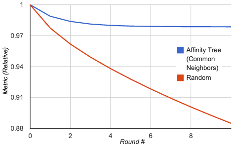
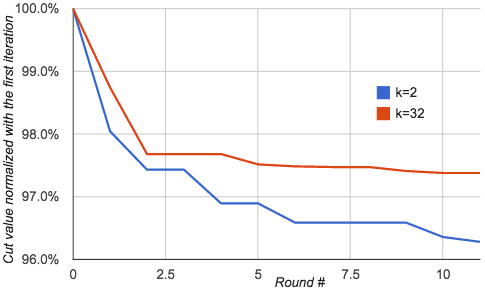
Figure 9: Convergence rate of Aff+Metric (top) and Aff+Swap (bottom) on World-roads.

6.3 Comparison to Previous Work

The most relevant among the previous work are the scalable label propagation-based algorithms of Ugander and Backstrom [UB13] and Martella et al. [MLS14]. The former reports their results on an internal graph (for Facebook) and a public social graph, LiveJournal, while the latter reports results on LiveJournal and Twitter. The cut sizes in the table for $k=40,60,80$ for [UB13] and all the numbers for [MLS14] are approximates taken from the graph provided in [UB13] as they do not report the exact values.The numbers in parentheses show the maximum imbalance in partition sizes, and the cut sizes are reported as fractions of total number of edges in the graph.

$k$ $\begin{subarray}{c}\mbox{\cite[cite]{[\@@bibref{}{wsdm-paper}{}{}]}}\\[-1.42262pt] (5\%)\end{subarray}$ $\begin{subarray}{c}\mbox{{Spinner}}\\ (5\%)\end{subarray}$ $\begin{subarray}{c}\mbox{{Aff}}\\ (0\%)\end{subarray}$ $\begin{subarray}{c}\mbox{{Combination}}\\ (0\%)\end{subarray}$ 20 37% 38% 35.71% 27.50% 40 43% 40% 40.83% 33.71% 60 46% 43% 43.03% 36.65% 80 47.5% 44% 43.27% 38.65% 100 49% 46% 45.05% 41.53%

Even our initial linear embedding (obtained by constructing the hierarchical clustering based on a weighted version of the input, where edge weights denote the number of common neighbors between two vertices) is consistently better than the best previous result. Our algorithm with the post-processing obtains $15\%$ to $25\%$ improvement over the previous results (better for smaller $k$), and it only requires a couple of post-processing rounds to converge. We take note that the results of [UB13] allow $5\%$ imbalance whereas our results produce almost perfectly balanced partitions.

Twitter is another public graph, for which the results of state-of-the-art minimum-cut partitioning is available. We report and compare the results of our main algorithm, Combination, for this graph to the best previous methods.

$k$ $\begin{subarray}{c}\mbox{\cite[cite]{[\@@bibref{}{SK12}{}{}]}}\\ (4-15\%)\end{subarray}$ $\begin{subarray}{c}\mbox{\tt Spinner}\\ (5\%)\end{subarray}$ $\begin{subarray}{c}\mbox{\tt FENNEL}\\ (10\%)\end{subarray}$ $\begin{subarray}{c}\mbox{\tt METIS}\\ (3\%)\end{subarray}$ $\begin{subarray}{c}\mbox{\small{Combination}}\\ (3\%)\end{subarray}$ 2 34% 15% 6.8% 11.98% 7.43% 4 55% 31% 29% 24.39% 18.16% 8 66% 49% 48% 35.96% 33.55% 16 76% 61% 59% N/A 46.18% 32 80% 69% 67% N/A 57.67%

Algorithms developed in [SK12, TGRV14] are suitable for the streaming model, but one can implement variants of those algorithms in a distributed manner. Our implementation of a natural distributed version of the FENNEL algorithm does not achieve the same results as those reported for the streaming implementation reported in [TGRV14]. However, we compare our algorithm directly to the numbers reported on Twitter by FENNEL [TGRV14].

Finally we report the cut sizes for another public graph, Friendster, so others can compare their results with it. The running time of our algorithms are not affected with large $k$; the running time difference for $k=2$ and tens of thousands is less than $1\%$, well within the noise associated with the distributed system. In fact, construction of the initial ordering is independent of $k$, and the post-processing steps may only take advantage of the increased parallelism possible for large $k$.

$k$ 2 10 $10^{2}$ Cut size 11.9% 41.4% 59.8%

We also make our partitions for Twitter, LiveJournal and Friendster publicly available [pub15].

6.4 Scalability

We noted above that the choice of $k$ does not affect the running time of the algorithm significantly: the running time for two and tens of thousands of partitions differed less than $1\%$ for Friendster.

As another measure of its scalability, we run the algorithm with $k=2$ on a series of random graphs (that are similar in nature) of varying sizes. In particular, we use RMAT graphs with parameter 20, 22, 24, 26 and 28, whose node and edge count is given in the table below. In addition, the last column gives the normalized running time of our algorithm on these graphs. Note that the size of the graph almost quadruples from one graph to the next.

graph $|V|$ $|E|$ max degree running time RMAT 20 650K 31M 65K 100% RMAT 22 2.4M 130M 160K 110% RMAT 24 8.9M 525M 400K 133% RMAT 26 32.8M 2.1B 1M 160% RMAT 28 120M 8.5B 2.5M 402%

6.5 Google Maps Driving Directions

As discussed in Section 1, we apply our results to the Google Maps Driving Directions application. Note that the evaluation metric for balanced partitioning of the world graph is the expected percentage of cross-shard queries over the total number of queries. More specifically, this objective function can be captured as follows: we first estimate the number of times each edge of graph may be part of the shortest path (or the driving direction) from the source to destination across all the query traffic. This produces an edge-weighted graph in which the weight of each edge is proportional to the number of times we expect this edge appearing in a driving direction, and our goal is to partition the graph into a small number of pieces and minimize the total weight of the edges cut. We can estimate each weight based on historical data and use it as a proxy for the number of times the edge appears on a driving direction on the real data. This objective is aligned with minimizing the weighted cut, and we can apply our algorithms to solve this problem.

Before deciding about our live experiments, we realized it might be suitable to use an imbalance factor in dividing the graph, and as a result, we first examined the best imbalance factor for our cut-optimization technique. The result of this study is summarized in Figure 10. In particular, we observe that we can reduce cross-shard queries by $21\%$ when increasing the imbalance factor from $0\%$ to $10\%$.

The two methods that we examined via live experiments were (i) a baseline approach based on the Hilbert-curve embedding, and (ii) one method based on applying our cut-optimization postprocessing techniques. Note that both these algorithms first compute an embedding of nodes into a line, which results in a much simpler system to identify the corresponding shards for the source and destination of each query at serving time. Finally, by running live experiments on the real traffic, we observe the number of multi-sharded queries from our cut-optimization techniques is almost 40$\%$ less than the number of multi-sharded queries compared to the naïve Hilbert embedding technique.

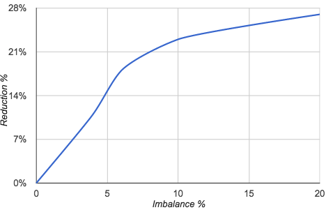
Figure 10: The percentage of improvement in cut value as we increase the allowable imbalance factor.

7 Conclusion

We develop a scalable algorithm for balanced partitioning of geographic and general graphs. The algorithm is based on embedding the vertices onto a line before chopping the sequence of vertices into almost equal pieces. The initial ordering obtained from hierarchical agglomerative clustering using the number of common neighbors as similarity measure outperforms the Hilbert cover-based partitioning even for geographic graphs. While the most effective postprocessing techniques are random-swap local improvements and minimum cut-based boundary optimization, iterative use of different techniques until convergence gives best overall results. Our algorithms improves upon the previously developed distributed balanced partitioning algorithms  [UB13, TGRV14, MLS14]. In addition, live experiments for the Google Maps Driving Direction shows significant advantage of our algorithm over a standard Hilbert curve-based partitioning.

Acknowledgements. The authors wish to thank Aaron Archer and Raimondas Kiveris for fruitful discussions.

References

- [AR06] Konstantin Andreev and Harald Räcke. Balanced graph partitioning. Theory Comput. Syst., 39(6):929–939, 2006.
- [BBLM14] MohammadHossein Bateni, Aditya Bhaskara, Silvio Lattanzi, and Vahab Mirrokni. Distributed balanced clustering via mapping coresets. In Advances in Neural Information Processing Systems 27: 28th Annual Conference on Neural Information Processing Systems 2014, 2014. To appear.
- [BEL13] Maria-Florina Balcan, Steven Ehrlich, and Yingyu Liang. Distributed clustering on graphs. In NIPS, page to appear, 2013.
- [BMV+12] Bahman Bahmani, Benjamin Moseley, Andrea Vattani, Ravi Kumar, and Sergei Vassilvitskii. Scalable -means++. PVLDB, 5(7):622–633, 2012.
- [BRSV11] Paolo Boldi, Marco Rosa, Massimo Santini, and Sebastiano Vigna. Layered label propagation: a multiresolution coordinate-free ordering for compressing social networks. In 20th Intl. Conf. on World Wide Web, (WWW), pages 587–596, 2011.
- [CHKR10] Moses Charikar, Mohammad Taghi Hajiaghayi, Howard J. Karloff, and Satish Rao. l spreading metrics for vertex ordering problems. Algorithmica, 56(4):577–604, 2010.
- [CK10] Avery Ching and Christian Kunz. Giraph : Large-scale graph processing on hadoop. In Hadoop Summit, 2010.
- [CKL+09] Flavio Chierichetti, Ravi Kumar, Silvio Lattanzi, Michael Mitzenmacher, Alessandro Panconesi, and Prabhakar Raghavan. On compressing social networks. In 15th ACM SIGKDD Intl. Conf. on Knowledge Discovery and Data Mining, pages 219–228, 2009.
- [DFF+03] Jack Dongarra, Ian Foster, Geoffrey Fox, William Gropp, Ken Kennedy, Linda Torczon, and Andy White. The Sourcebook of Parallel Computing. Morgan Kaufmann Publishers Inc., San Francisco, CA, USA, 2003.
- [DG04] Jeffrey Dean and Sanjay Ghemawat. Mapreduce: Simplified data processing on large clusters. In OSDI, pages 137–150, 2004.
- [DGRW11] Daniel Delling, Andrew V. Goldberg, Ilya Razenshteyn, and Renato Fonseca F. Werneck. Graph partitioning with natural cuts. In 25th IEEE International Symposium on Parallel and Distributed Processing, IPDPS 2011, pages 1135–1146, 2011.
- [DGRW12] Daniel Delling, Andrew V. Goldberg, Ilya Razenshteyn, and Renato Fonseca F. Werneck. Exact combinatorial branch-and-bound for graph bisection. In Proceedings of the 14th Meeting on Algorithm Engineering & Experiments, ALENEX 2012, pages 30–44, 2012.
- [EIM11] Alina Ene, Sungjin Im, and Benjamin Moseley. Fast clustering using mapreduce. In KDD, pages 681–689, 2011.
- [FK02] Uriel Feige and Robert Krauthgamer. A polylogarithmic approximation of the minimum bisection. SIAM J. Comput., 31(4):1090–1118, 2002.
- [FL07] Uriel Feige and James R. Lee. An improved approximation ratio for the minimum linear arrangement problem. Inf. Process. Lett., 101(1):26–29, 2007.
- [FTW00] Peter C. Fishburn, Prasad Tetali, and Peter Winkler. Optimal linear arrangement of a rectangular grid. Discrete Mathematics, 213(1-3):123–139, 2000.
- [GH88] Olivier Goldschmidt and Dorit S. Hochbaum. Polynomial algorithm for the k-cut problem. In 29th Annual Symposium on Foundations of Computer Science, FOCS 1988, pages 444–451, 1988.
- [GJ79a] M. R. Garey and D. S. Johnson. Computers and Intractability: A Guide to the Theory of NP-Completeness. W.H. Freeman and Company, 1979.
- [GJ79b] M. R. Garey and David S. Johnson. Computers and Intractability: A Guide to the Theory of NP-Completeness. W. H. Freeman, 1979.
- [GL96] Craig Gotsman and Michael Lindenbaum. On the metric properties of discrete space-filling curves. IEEE Transactions on Image Processing, 5(5):794–797, 1996.
- [KK98] George Karypis and Vipin Kumar. A fast and high quality multilevel scheme for partitioning irregular graphs. SIAM J. Sci. Comput., 20(1):359–392, 1998.
- [KLM+14] Raimondas Kiveris, Silvio Lattanzi, Vahab Mirrokni, Vibhor Rastogi, and Sergei Vassilvitskii. Connected components in mapreduce and beyond. In Fifth ACM Symposium on Cloud Computing, SOCC 2014, 2014.
- [KLPM10] Haewoon Kwak, Changhyun Lee, Hosung Park, and Sue Moon. What is Twitter, a social network or a news media? In WWW ’10: Proceedings of the 19th international conference on World wide web, pages 591–600, New York, NY, USA, 2010. ACM.
- [KTF09] U. Kang, Charalampos E. Tsourakakis, and Christos Faloutsos. PEGASUS: A Peta-Scale Graph Mining System- Implementation and Observations. 2009.
- [MAB+10] Grzegorz Malewicz, Matthew H. Austern, Aart J.C Bik, James C. Dehnert, Ilan Horn, Naty Leiser, and Grzegorz Czajkowski. Pregel: a system for large-scale graph processing. In SIGMOD, 2010.
- [MJFS01] Bongki Moon, H. V. Jagadish, Christos Faloutsos, and Joel H. Saltz. Analysis of the clustering properties of the hilbert space-filling curve. IEEE Transactions on Knowledge and Data Engineering, 13:2001, 2001.
- [MLS14] Claudio Martella, Dionysios Logothetis, and Georgos Siganos. Spinner: Scalable graph partitioning for the cloud. CoRR, abs/1404.3861, 2014.
- [NRS02] Rolf Niedermeier, Klaus Reinhardt, and Peter Sanders. Towards optimal locality in mesh-indexings. Discrete Applied Mathematics, 117(1-3):211–237, 2002.
- [pub15] Public data for balanced partioning paper. http://goo.gl/okvwpa, 2015.
- [RMCS13] Vibhor Rastogi, Ashwin Machanavajjhala, Laukik Chitnis, and Anish Das Sarma. Finding connected components in map-reduce in logarithmic rounds. In 29th IEEE International Conference on Data Engineering, ICDE 2013, pages 50–61, 2013.
- [RR04] Satish Rao and Andréa W. Richa. New approximation techniques for some linear ordering problems. SIAM J. Comput., 34(2):388–404, 2004.
- [SK12] Isabelle Stanton and Gabriel Kliot. Streaming graph partitioning for large distributed graphs. In The 18th ACM SIGKDD International Conference on Knowledge Discovery and Data Mining, KDD ’12, pages 1222–1230, 2012.
- [SM58] R. R. Sokal and C. D. Michener. A statistical method for evaluating systematic relationships. University of Kansas Science Bulletin, 38:1409–1438, 1958.
- [SS00] Roman G. Strongin and Yaroslav D. Sergeyev. Global optimization with non-convex constraints: sequential and parallel algorithms. Nonconvex Optimization and Its Applications. Kluwer academic publishers, Dordrecht, Boston, Londres, 2000.
- [Sta14] Isabelle Stanton. Streaming balanced graph partitioning algorithms for random graphs. In Proceedings of the Twenty-Fifth Annual ACM-SIAM Symposium on Discrete Algorithms, SODA 2014, pages 1287–1301, 2014.
- [TGRV14] Charalampos E. Tsourakakis, Christos Gkantsidis, Bozidar Radunovic, and Milan Vojnovic. FENNEL: streaming graph partitioning for massive scale graphs. In Seventh ACM International Conference on Web Search and Data Mining, WSDM 2014, pages 333–342, 2014.
- [TKM09] Charalampos E. Tsourakakis, Mihail N. Kolountzakis, and Gary L. Miller. Approximate triangle counting. CoRR, abs/0904.3761, 2009.
- [UB13] Johan Ugander and Lars Backstrom. Balanced label propagation for partitioning massive graphs. In WSDM, pages 507–516, 2013.
- [YCLN14] Da Yan, James Cheng, Yi Lu, and Wilfred Ng. Blogel: A block-centric framework for distributed computation on real-world graphs. PVLDB, 7(14):1981–1992, 2014.