Decay of bound states in the continuum of Majorana fermions induced by vacuum fluctuations: Proposal of qubit technology

Abstract

We report on a theoretical investigation of the interplay between vacuum fluctuations, Majorana quasiparticles (MQPs) and bound states in the continuum (BICs) by proposing a new venue for qubit storage. BICs emerge due to quantum interference processes as the Fano effect and, since such a mechanism is unbalanced, these states decay as regular into the continuum. Such fingerprints identify BICs in graphene as we have discussed in detail in Phys. Rev. B 92, 245107 and 045409 (2015). Here by considering two semi-infinite Kitaev chains within the topological phase, coupled to a quantum dot (QD) hybridized with leads, we show the emergence of a novel type of BICs, in which MQPs are trapped. As the MQPs of these chains far apart build a delocalized fermion and qubit, we identify that the decay of these BICs is not connected to Fano and it occurs when finite fluctuations are observed in the vacuum composed by electron pairs for this qubit. From the experimental point of view, we also show that vacuum fluctuations can be induced just by changing the chain-dot couplings from symmetric to asymmetric. Hence, we show how to perform the qubit storage within two delocalized BICs of MQPs and to access it when the vacuum fluctuates by means of a complete controllable way in quantum transport experiments.

I Introduction

An astonishing aftermath in the underlying framework of quantum theory is the possibility of fluctuations within the corresponding quantum field describing the vacuum, in which pairs of virtual particles pop up leading to counterintuitive phenomena. In this regard, the Casimir effect Casimir is the most known picture in Physics arising from the straight outcome of vacuum fluctuations. In particular, the Casimir effect manifests itself as an attractive force between two reflecting, plane and parallel plates, even when external fields are entirely absent.

On the ground of condensed matter Physics, we make explicit that the interplay between vacuum fluctuations and Majorana quasiparticles (MQPs) Franz is accomplishable by the setup proposed in Fig. 1, where we find peculiar bound states in the continuum (BICs) Neuman for a pair of semi-infinite Kitaev chains Franz ; UFMG ; Nayana ; Jelena ; Vernek1 ; Vernek2 in the topological phase and coupled to a quantum dot (QD) connected to leads. Concerning on BICs, they were pioneering predicted by von Neumann and Wigner in 1929 Neuman as quantum states for electrons described by localized square-integrable wave functions appearing in the continuum of those delocalized and exhibiting infinite lifetimes for such electrons. Hence, electrons within BICs do not decay into the continuum acting as fully invisible states from the perspective of conductance measurements. The issue on BICs had a revival after the works of Stillinger and Herrick in 1975 SH , followed by the experimental realization made by Capasso and co-workers in 1992, concerning semiconductor heterostructures Capasso . Noteworthy, BICs are expected to emerge in several systems as in graphene QPT ; BIC1 ; Gong , optics and photonics BIC2 ; BIC3 ; Exp1 ; Exp2 , setups characterized by singular chirality Chiral , Floquet-Hubbard states due to strong oscillating electric field Floquet and driven by A.C. fields AC .

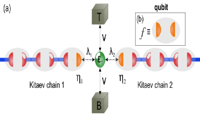
Figure 1: (Color online) For a off-resonance QD with the Fermi level of the top (T) and bottom (B) leads, together with couplings $\lambda_{1}=\lambda_{2},$ BICs of the MQPs $\eta_{1}$ and $\eta_{2}$ emerge. $V$ is the hybridization of the QD with the leads. The vacuum of electron pairs for the quibt $f$ fluctuates when $\lambda_{1}\equiv(t+\Delta)\neq\lambda_{2}\equiv(t-\Delta),$ thus inducing the decay of the BICs into the system continuum of energies.

In this paper, we show that the setup proposed in Fig. 1 enables the observation of an unprecedented phenomenon: vacuum fluctuations yielding the decay of BICs into the continuum, in which the building blocks of the former are MQPs for qubit storage. We highlight two setups considered proper platforms for MQPs in Kitaev chains as well as for the experimental achievement of our proposal: i) an $s$-wave superconductor nearby a semiconducting nanowire where two magnetic fields exist perpendicular to each other, wherein one of them arises from the spin-orbit coupling of the semiconductor, while the second is applied externally to freeze the spin degree of freedom of the system and to ensure topological superconductivity wire1 , and ii) magnetic chains on top of superconductors characterized by a strong spin-orbit parameter wire2 ; Jelena2 . Moreover, MQPs are expected to rise among several setups as the fractional quantum Hall state with filling factor $\nu=5/2$ QH , in three-dimensional topological insulators TI and at the center of superconducting vortices as well V1 ; V2 ; V3 .

To the best of our knowledge, the works up to date published in the literature have focused mainly on BICs assisted by Fano interference QPT ; BIC1 ; BIC2 ; BIC3 . The so-called Fano effect is a quantum inference phenomenon, wherein transport channels compete for the electron tunneling, mainly via a continuum of energies hybridized with discrete levels of nanoscale structures Fano1 ; Fano . Here, as an alternative we propose that quantum fluctuations in the vacuum of electron pairs arising from the regular fermion and qubit $f$ composed by the MQPs $\eta_{1}=\eta_{1}^{\dagger}$ and $\eta_{2}=\eta_{2}^{\dagger}$, cf. shown in Fig.1, give rise to the decay of these peculiar BICs, the so-called quasi BICs. Otherwise, the BICs of MQPs remain intact.

In order to present our proposal in a comprehensive way, we begin by defining the qubit $f$ as follows: $f=\frac{1}{\sqrt{2}}(\eta_{1}+i\eta_{2})$ and $f^{\dagger}=\frac{1}{\sqrt{2}}(\eta_{1}-i\eta_{2}),$ in which the occupations

$$<f^{\dagger}f^{\dagger}>=\int_{-\infty}^{+\infty}d\varepsilon\text{{DO$S_{f^{\dagger}f^{\dagger}}$}}=<ff>=\int_{-\infty}^{+\infty}d\varepsilon\text{{DO$S_{ff}$}}$$

$$=0$$ (1)

can be found book , here expressed in terms of the densities DO$S_{f^{\dagger}f^{\dagger}}$ and DO$S_{ff}$, since the pairings $f^{\dagger}f^{\dagger}$ and $ff$ are not allowed in the system when both the Kitaev chains considered are equally coupled to the QD. Later on, such densities will be deduced from our model Hamiltonian. Furthermore, we will clarify that vacuum fluctuations can be tunable experimentally. To that end, we should take into account asymmetric Kitaev chain-dot couplings and a off-resonance QD with the Fermi level of the leads, since the symmetric case prevents vacuum fluctuations thus ensuring the qubit storage as MQPs delocalized at the edges of the Kitaev chains as sketched in Fig. 1. Hence, by means of BICs of MQPs, we propose a novel manner of qubit storage when a single QD and controllable vacuum fluctuations are accounted.

II The Model

To give a theoretical description of the setup depicted in Fig. 1 describing two semi-infinite Kitaev chains within the topological phase and connected to a QD coupled to leads, we employ an extension of the Hamiltonian inspired on the original proposal from Liu and Baranger, which is a spinless model to ensure topological superconductivity Ref. [Baranger, ]:

$$\mathcal{H} = \underset{\alpha k}{\sum}\tilde{\varepsilon}_{\alpha k}c_{\alpha k}^{\dagger}c_{\alpha k}+\varepsilon_{1}d_{1}^{\dagger}d_{1}+V\underset{\alpha k}{\sum}(c_{\alpha k}^{\dagger}d_{1}+\text{{H.c.}})$$ (2)

$$+ \frac{(t+\Delta)}{\sqrt{2}}(d_{1}-d_{1}^{\dagger})\eta_{1}+i\frac{(\Delta-t)}{\sqrt{2}}(d_{1}+d_{1}^{\dagger})\eta_{2},$$

where the electrons in the lead $\alpha=T,B$ are described by the operator $c_{\alpha k}^{\dagger}$ ($c_{\alpha k}$) for the creation (annihilation) of an electron in a quantum state labeled by the wave number $k$ and energy $\tilde{\varepsilon}_{\alpha k}=\varepsilon_{k}-\mu_{\alpha}$, with $\mu_{\alpha}$ as the chemical potential. For the QD coupled to leads, $d_{1}^{\dagger}$ ($d_{1}$) creates (annihilates) an electron in the state $\varepsilon_{1}.$ $V$ stands for the hybridizations between the QD and the leads. The QD couples asymmetrically to the Kitaev chains with tunneling amplitudes proportional to $(t+\Delta)\equiv\lambda_{1}$ and $(t-\Delta)\equiv\lambda_{2},$ respectively for the left and right MQPs $\eta_{1}$ and $\eta_{2}.$ We stress that the prefactors $1/\sqrt{2}$ and $i/\sqrt{2},$ respectively for $\lambda_{1}$ and $\lambda_{2}$ constitute a convenient gauge that changes the last two terms of Eq. (2) into $td_{1}f^{\dagger}-td_{1}^{\dagger}f+\Delta f^{\dagger}d_{1}^{\dagger}-\Delta fd_{1}=td_{1}f^{\dagger}+\Delta f^{\dagger}d_{1}^{\dagger}+\text{{H.c.}},$ when the representation $f$ is adopted. As a result, we can notice that the electrons within $f$ and $d_{1}$ beyond the normal tunneling $t$ between them, become bounded as a Cooper pair with binding energy $\Delta.$ Particularly, with $\Delta\neq 0$ we will verify that the BICs here proposed decay into the continuum due to the emergence of these paring terms.

In what follows, we use the Landauer-Büttiker formula for the zero-bias conductance $G$ Baranger . Such a quantity is given by:

$$G=\frac{e^{2}}{h}\Gamma\int d\varepsilon\left(\frac{\partial f_{F}}{\partial\varepsilon}\right)\text{{Im}}(\tilde{\mathcal{G}}_{d_{1}^{\dagger}d_{1}}),$$ (3)

where $\Gamma=2\pi V^{2}\sum_{k}\delta(\varepsilon-\varepsilon_{k})$ is the Anderson broadening Anderson , $f_{F}$ stands for the Fermi-Dirac distribution, $\tilde{\mathcal{G}}_{d_{1}^{\dagger}d_{1}}$ is the retarded Green’s function for the QD in energy domain $\varepsilon,$ obtained from the time Fourier transform of $\tilde{\mathcal{G}}_{\mathcal{B^{\dagger}\mathcal{A}}}=\int d\tau\mathcal{G}_{\mathcal{B^{\dagger}\mathcal{A}}}e^{\frac{i}{\hbar}(\varepsilon+i0^{+})\tau}.$ Furthermore, we introduced $\mathcal{T}=-\Gamma\text{{Im}}(\tilde{\mathcal{G}}_{d_{1}^{\dagger}d_{1}})$ as the transmittance through the QD. $\mathcal{G}_{\mathcal{B^{\dagger}\mathcal{A}}}=-\frac{i}{\hbar}\theta(\tau){\tt Tr}\{\varrho[\mathcal{A}(\tau),\mathcal{B}^{\dagger}(0)]_{+}\}$ corresponds to the Green’s function in time domain $\tau,$ here expressed in terms of the density matrix $\varrho$ for Eq. (2) and the Heaviside function $\theta\left(\tau\right).$ From $\mathcal{G}_{\mathcal{B^{\dagger}\mathcal{A}}},$ it is possible to find the expectation value $<\mathcal{B^{\dagger}\mathcal{A}}>=\int d\varepsilon\text{{DO$S_{\mathcal{B^{\dagger}\mathcal{A}}}$}}$ by using $\text{{DO$S_{\mathcal{B^{\dagger}\mathcal{A}}}$}}=-\frac{1}{\pi}\text{{Im}}(\mathcal{G}_{\mathcal{B^{\dagger}\mathcal{A}}})$ as the corresponding density of states, similarly to Eq. (1) for the vacuum. Particularly for Eq. (3), we used $\mathcal{A=B}=d_{1}$ and to calculate $\tilde{\mathcal{G}}_{d_{1}^{\dagger}d_{1}}$ together with other Green’s functions, we should employ the equation-of-motion (EOM) method book summarized as follows: $\omega\tilde{\mathcal{G}}_{B^{\dagger}\mathcal{A}}=(\varepsilon+i0^{+})\tilde{\mathcal{G}}_{B^{\dagger}\mathcal{A}}=[\mathcal{A},\mathcal{B^{\dagger}}]_{+}+\tilde{\mathcal{G}}_{\mathcal{B}^{\dagger}\left[\mathcal{A},\mathcal{\mathcal{H}}\right]}.$ As a result, we find

$$(\varepsilon-\varepsilon_{1}+i\Gamma)\tilde{\mathcal{G}}_{d_{1}^{\dagger}d_{1}}=1-t\mathcal{\tilde{G}}_{d_{1}^{\dagger},f}-\Delta\mathcal{\tilde{G}}_{d_{1}^{\dagger},f^{\dagger}},$$ (4)

in addition to the Green’s functions $\mathcal{\tilde{G}}_{d_{1}^{\dagger},f}$ and $\mathcal{\tilde{G}}_{d_{1}^{\dagger},f^{\dagger}}.$ According to the EOM approach, we also have $\omega\mathcal{\tilde{G}}_{d_{1}^{\dagger},f}=(\Delta\mathcal{\tilde{G}}_{d_{1}^{\dagger},d_{1}^{\dagger}}-t\mathcal{\tilde{G}}_{d_{1}^{\dagger},d_{1}}),$ $\omega\mathcal{\tilde{G}}_{d_{1}^{\dagger},f^{\dagger}}=(t\mathcal{\tilde{G}}_{d_{1}^{\dagger},d_{1}^{\dagger}}-\Delta\mathcal{\tilde{G}}_{d_{1}^{\dagger},d_{1}})$ and $\mathcal{\tilde{G}}_{d_{1}^{\dagger},d_{1}^{\dagger}}=-2t\Delta\tilde{K}\mathcal{\tilde{G}}_{d_{1}^{\dagger},d_{1}},$ in which $\tilde{K}=[\varepsilon+\varepsilon_{1}-K(t,\Delta)+i\Gamma]^{-1}K,$ $K(t,\Delta)=[\varepsilon^{2}+2i\varepsilon 0^{+}-(0^{+})^{2}]^{-1}\omega(t^{2}+\Delta^{2})$ and $K=[\varepsilon^{2}+2i\varepsilon 0^{+}-(0^{+})^{2}]^{-1}\omega.$ Consequently, the Green’s function of the QD reads

$$\tilde{\mathcal{G}}_{d_{1}^{\dagger}d_{1}} =\frac{1}{\varepsilon-\varepsilon_{1}+i\Gamma-\Sigma_{\text{{MQPs}}}},$$ (5)

where $\Sigma_{\text{{MQPs}}}=K(t,\Delta)+(2t\Delta)^{2}K\tilde{K}$ accounts for the self-energy due to the MQPs connected to the QD and $\text{{DOS}}_{11}=-\frac{1}{\pi}\text{{Im}}(\tilde{\mathcal{G}}_{d_{1}^{\dagger}d_{1}})$ is the density of states for the QD. Particularly for $t=\Delta=\frac{\lambda}{\sqrt{2}},$ the expressions for $\tilde{K}$ and $\Sigma_{\text{{MQPs}}}$ found in Ref. [Baranger, ] are recovered.

To perceive the emergence of BICs in the Kitaev chains and vacuum fluctuations, we need to find the densities for the MQPs $\eta_{1}$ and $\eta_{2},$ namely $\text{{DOS}}_{\eta_{1}}=-\frac{1}{\pi}\text{{Im}}(\tilde{\mathcal{G}}_{\eta_{1}\eta_{1}})$ and $\text{{DOS}}_{\eta_{2}}=-\frac{1}{\pi}\text{{Im}}(\tilde{\mathcal{G}}_{\eta_{2}\eta_{2}}),$ together with $\text{{DOS}}_{ff}=-\frac{1}{\pi}\text{{Im}}(\tilde{\mathcal{G}}_{ff})$ and $\text{{DOS}}_{f^{\dagger}f^{\dagger}}=-\frac{1}{\pi}\text{{Im}}(\tilde{\mathcal{G}}_{f^{\dagger}f^{\dagger}}),$ in which the latter allows to determine the occupations $<f^{\dagger}f^{\dagger}>$ and $<ff>$ as Eq. (1) ensures for the vacuum of electron pairs. Thus the EOM gives rise to

$$\mathcal{\tilde{G}}_{\eta_{1}\eta_{1}} = \frac{1}{2}(\mathcal{\tilde{G}}_{f^{\dagger}f^{\dagger}}+\mathcal{\tilde{G}}_{ff^{\dagger}}+\mathcal{\tilde{G}}_{f^{\dagger}f}+\mathcal{\tilde{G}}_{ff})$$ (6)

and

$$\mathcal{\tilde{G}}_{\eta_{2}\eta_{2}} = \frac{1}{2}(-\mathcal{\tilde{G}}_{f^{\dagger}f^{\dagger}}+\mathcal{\tilde{G}}_{ff^{\dagger}}+\mathcal{\tilde{G}}_{f^{\dagger}f}-\mathcal{\tilde{G}}_{ff})$$ (7)

for the Green’s functions of the MQPs, with

$$\omega\tilde{\mathcal{G}}_{f^{\dagger}f^{\dagger}}=(t\tilde{\mathcal{G}}_{f^{\dagger}d_{1}^{\dagger}}-\Delta\mathcal{G}_{f^{\dagger}d_{1}})$$ (8)

and

$$\omega\tilde{\mathcal{G}}_{ff}=(-t\tilde{\mathcal{G}}_{fd_{1}}+\Delta\tilde{\mathcal{G}}_{fd_{1}^{\dagger}})$$ (9)

for those describing the aforementioned vacuum. To close the system of Green’s functions above-described, we calculate via EOM the following $\omega\tilde{\mathcal{G}}_{ff^{\dagger}}=(1+t\tilde{\mathcal{G}}_{fd_{1}^{\dagger}}-\Delta\mathcal{G}_{fd_{1}}),$ $\omega\tilde{\mathcal{G}}_{f^{\dagger}f}=(1-t\tilde{\mathcal{G}}_{f^{\dagger}d_{1}}+\Delta\tilde{\mathcal{G}}_{f^{\dagger}d_{1}^{\dagger}}),$ $\omega\tilde{\mathcal{G}}_{f^{\dagger}d_{1}}=-t(1+2\Delta^{2}\tilde{K})\tilde{\mathcal{G}}_{d_{1}^{\dagger}d_{1}},$ $\omega\tilde{\mathcal{G}}_{fd_{1}}=-\Delta(1+2t^{2}\tilde{K})\tilde{\mathcal{G}}_{d_{1}^{\dagger}d_{1}},$ $\tilde{\mathcal{G}}_{f^{\dagger}d_{1}^{\dagger}}=\Delta\tilde{K}K^{-1}\omega^{-1}-2t\Delta\tilde{K}\mathcal{G}_{f^{\dagger}d_{1}}$ and $\tilde{\mathcal{G}}_{fd_{1}^{\dagger}}=t\tilde{K}K^{-1}\omega^{-1}-2t\Delta\tilde{K}\mathcal{G}_{fd_{1}}.$

Thus based on the theoretical framework developed up to here, shortly thereafter we will discuss the role of Eqs.(5), (6) and (7) in the connection with the novel qubit technology proposed in this paper.

III Results and Discussion

In the simulations discussed here we adopt $T=0$ and the Anderson broadening $\Gamma=2\pi V^{2}\sum_{k}\delta(\varepsilon-\varepsilon_{k})$ as the energy scale for the parameters from the system Hamiltonian of Eq. (2). In order to make explicit the phenomenon of qubit storage ruled by vacuum fluctuations, due to the Kitaev chains connected to the QD, we should begin by analyzing the cases in which both are decoupled from each other $(\lambda_{1}=\lambda_{2}=0)$. Within this situation, but for the QD in resonance with the Fermi level of the metallic leads $(\varepsilon_{1}=\varepsilon_{F}\equiv 0),$ the standard Lorentzian shape depicted in Fig. 2(a) for the DOS encoded by $\text{{DOS}}_{11}=-\frac{1}{\pi}\text{{Im}}(\tilde{\mathcal{G}}_{d_{1}^{\dagger}d_{1}})$ as a function of energy $\varepsilon$ is verified. In the panel (b) of the same figure, we find coincident profiles for $\text{{DOS}}_{\eta_{1}}=-\frac{1}{\pi}\text{{Im}}(\tilde{\mathcal{G}}_{\eta_{1}\eta_{1}})$ and $\text{{DOS}}_{\eta_{2}}=-\frac{1}{\pi}\text{{Im}}(\tilde{\mathcal{G}}_{\eta_{2}\eta_{2}})$ describing the DOSs of the MQPs, respectively found at the edges of the Kitaev chains $1$ and $2$ nearby the QD. Once the MQPs are zero-energy modes for discrete states, the curves of $\text{{DOS}}_{\eta_{1}}$ and $\text{{DOS}}_{\eta_{2}}$ are indeed Dirac delta functions as expected, due to the absence of leads connected to the Kitaev chains. These Delta functions represent the complete storage of the qubit $f$ composed by the MQPs $\eta_{1}$ and $\eta_{2},$ since the zero broadening of such DOSs point out that the electron within $f$ has an infinite lifetime and does not decay into the QD. Below, we will see that such a scenario is modified when the Kitaev chain-QD couplings are turned-on, i.e., $\lambda_{1}=\lambda_{2}\neq 0$.

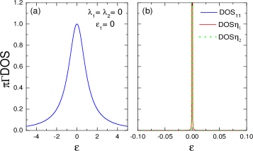
Figure 2: (Color online) (a) DOS of the QD in resonance with the Fermi level of the leads $(\varepsilon_{F}\equiv 0)$ when the Kitaev chains are absent: a Lorentzian shape is observed. (b) DOSs of the MQPs by neglecting the couplings to the leads: a Delta function profile appears instead. Details in the main text.

Fig. 3(a) treats the symmetric regime $\lambda_{1}=\lambda_{2}=10\Gamma,$ in which the QD is still in resonance with the leads Fermi level. As both the QD and MQPs are zero-energy modes and share the same DOS profile $(\text{{DOS}}_{\eta_{1}}=\text{{DOS}}_{\eta_{2}}=\text{{DOS}}_{11}),$ the outcome of this set is to exhibit the same splitting of the zero-peak, which was originally centered at the Fermi energy as showed in Figs.2(a) and (b). Once the zero-peak is splitted, one can propose a manner of controlling this splitting within the $\text{{DOS}}_{11}.$ The way we have found is by placing the QD off-resonance in respect with the leads Fermi level. This picture can be visualized in Fig. 3(b) for the dashed-red curve with $\varepsilon_{1}=-\Gamma,$ where we can perceive the red and blue shifts of the peaks. On the other hand, the response of the MQPs due to the tuning of $\varepsilon_{1}$ is fully different compared to the QD: the original pattern given by a pair of peaks for the MQPs appearing in Fig. 3(a) evolves towards a novel structure, where four peaks emerge as depicted by the dotted and solid blue curves of Fig. 3(b). Note that this novel pattern is not well resolved for $\varepsilon_{1}=-\Gamma$ yet, since the peaks within each pair of peaks are found partially merged. However, if we consider $\varepsilon_{1}=-2.5\Gamma$ as in Fig. 3(c), the visibility of the four peaks becomes more pronounced and they appear completely resolved. We should draw attention in the manner that the pairs of peaks in the DOSs for the MQPs evolve from the pattern observed in Fig. 3(b) to that in panel (c). To reveal the underlying mechanism of such an electron-hole asymmetry, we should focus on panels (a)-(c) of Fig. 4 and, in particular, Eqs.(6) and (7) for $\text{{DOS}}_{\eta_{1}}=-\frac{1}{\pi}\text{{Im}}(\tilde{\mathcal{G}}_{\eta_{1}\eta_{1}})$ and $\text{{DOS}}_{\eta_{2}}=-\frac{1}{\pi}\text{{Im}}(\tilde{\mathcal{G}}_{\eta_{2}\eta_{2}}),$ respectively.

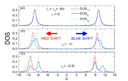
Figure 3: (Color online) (a) Scenario of Figs.2(a) and (b) modified when the Kitaev chain-QD symmetric couplings are turned-on: as the QD and the MQPs are in resonance, their DOSs split equally. (b) For the QD off-resonance, a new structure composed by four peaks emerges only in the DOSs for the MQPs. (c) Visualization of the red and blue shifts of the peaks found in (b) by placing the QD very far from the resonance.

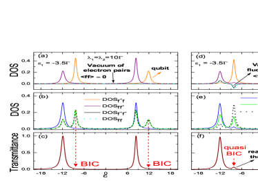
Figure 4: (Color online) Symmetric regime of Kitaev chain-QD couplings: (a) DOSs for electrons within the qubit $f$ and absence of vacuum fluctuations outlined by the vertical arrow; (b) DOSs for the QD and MQPs in absence of vacuum fluctuations; (c) transmittance profile with BICs appearing denoted by dashed-vertical arrows, i.e., the lacking of the corresponding peaks found at the same positions within panel (b) for the DOSs of the MQPs is a BIC fingerprint, since these states do not contribute to the quantum transport. Only the peaks of the DOS for the QD remain in the transmittance. Asymmetric regime of Kitaev chain-QD couplings: (d) the vacuum fluctuates around the BICs verified in (c) and the DOSs for $f$ also change; (e) DOSs for the QD and MQPs in presence of vacuum fluctuations; (f) As aftermath of the fluctuations observed in (d) which are denoted by arrows, the BICs of MQPs found in panel (c) decay as quasi BICs. They are found outlined by dashed-vertical arrows as we can visualize in the transmittance profile.

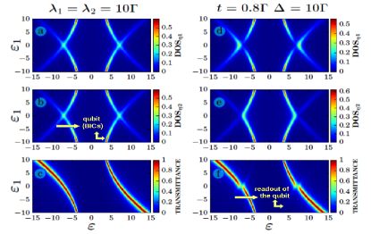
Figure 5: (Color online) Symmetric regime of Kitaev chain-QD couplings: in panels (a), (b) and (c) we see the density plots of the DOSs for the MQPs and transmittance spanned by the axis $\varepsilon_{1}$ and $\varepsilon.$ Panel (c) for the transmittance shows only two bows from the set of four bows found in (a) and (b) describing the DOSs of the MQPs. The lack of such bows in the transmittance then denotes BICs of MQPs. Asymmetric regime of Kitaev chain-QD couplings: panels (d) and (e) are similar to (a) and (b), but in panel (f) quasi BICs appear as light bows in the transmittance in respect with those verified in panels (d) and (e).

Still in the symmetric regime $\lambda_{1}=\lambda_{2}=10\Gamma,$ we see that only $\mathcal{\tilde{G}}_{ff^{\dagger}}$ and $\mathcal{\tilde{G}}_{f^{\dagger}f}$ rise in Fig. 4(a) respectively via the $\text{{DOS}}_{ff^{\dagger}}=-\frac{1}{\pi}\text{{Im}}(\tilde{\mathcal{G}}_{ff^{\dagger}})$ and $\text{{DOS}}_{f^{\dagger}f}=-\frac{1}{\pi}\text{{Im}}(\tilde{\mathcal{G}}_{f^{\dagger}f})$, while $\mathcal{\tilde{G}}_{f^{\dagger}f^{\dagger}}$ and $\mathcal{\tilde{G}}_{ff}$ contributes with $\text{{DOS}}_{f^{\dagger}f^{\dagger}}=\text{{DOS}}_{ff}=0$ as aftermath of the vacuum $<f^{\dagger}f^{\dagger}>=<ff>=0$ for the electron pairs. Besides, the structure of four peaks firstly displayed in Fig. 3(c) and together with Fig. 4(b) for the MQPs $\eta_{1}$ and $\eta_{2}$ considering $\varepsilon_{1}=-3.5\Gamma,$ then make explicit that the unmatched profiles of the $\text{{DOS}}_{ff^{\dagger}}$ and $\text{{DOS}}_{f^{\dagger}f}$ play the role of two spectral functions analogous to the possibilities $\text{{DOS}}_{\uparrow}$ and $\text{{DOS}}_{\downarrow},$ due to spin-imbalance in ferromagnetic systems. Based on this, we can realize the features within Fig. 4(c), where the peaks appearing in the transmittance $\mathcal{T}=-\Gamma\text{{Im}}(\tilde{\mathcal{G}}_{d_{1}^{\dagger}d_{1}})$ determined by Eq.(3) do not correspond to those found in panel (a) for the $\text{{DOS}}_{f^{\dagger}f},$ but just to those from $\text{{DOS}}_{ff^{\dagger}}.$ Equivalently, from those four peaks observed in Fig. 4(b) for the MQPs, solely two of them decay into the QD, thus contributing to the conductance. As a result, the peaks within $\text{{DOS}}_{\eta_{1}}=\text{{DOS}}_{\eta_{2}}$ that do not appear in $\mathcal{T}$ correspond to BICs of MQPs, which constitute the building blocks of the delocalized qubit $f$ characterized by the two peaks found in Fig. 4(a) for the $\text{{DOS}}_{f^{\dagger}f}.$ These invisible peaks arising from the $\text{{DOS}}_{f^{\dagger}f}$ in $\mathcal{T}$, then provide a novel manner of qubit storage, wherein despite the coupling $\lambda_{1}=\lambda_{2}=10\Gamma$ of the Kitaev chains with the QD, the decay of the state $f$ is completely prevented. Such a forbiddance, we should highlight, occurs when the vacuum $<f^{\dagger}f^{\dagger}>=<ff>=0$ does not fluctuate [Fig. 4(a)]. In what follows, we will show that when $<f^{\dagger}f^{\dagger}>=<ff>\neq 0,$ just in the vicinity of BICs, the suppression of the qubit storage occurs and hence, the decay of the BICs as quasi BICs is allowed appearing thought out the transmittance.

To fluctuate the vacuum considered, it is demanded asymmetric couplings $\lambda_{1}\neq\lambda_{2}$ by means of $\Delta=10\Gamma$ and $t=0.8\Gamma,$ for instance. As a net effect we have $\text{{DOS}}_{f^{\dagger}f^{\dagger}}=\text{{DOS}}_{ff}\neq 0$ corresponding to fluctuations in the vacuum $<f^{\dagger}f^{\dagger}>=<ff>\neq 0$ around the BICs, which appear pointed out by black arrows in Fig. 4(d). In such a situation, pairing terms $d_{1}f+f^{\dagger}d_{1}^{\dagger}$ appear, which allow the correlations above to become finite. Consequently, the profiles for $\text{{DOS}}_{\eta_{1}}$ and $\text{{DOS}}_{\eta_{2}}$ become distinct as showed in Fig. 4(e), resulting in the detection of the BICs by means of the quasi BICs, which appear as unpronounced states indicated by dashed-red arrows in Fig. 4(f). Noteworthy, the quasi BICs are placed exactly at the positions of the BICs found in Fig. 4(c). Moreover, it is worth noticing in opposite to the unbalance of Fano interference as the underlying mechanism for the rising of quasi BICs reported in graphene systems QPT ; BIC1 , here we identify that vacuum fluctuations of the electron pairs described by the expectation value $<f^{\dagger}f^{\dagger}>=<ff>\neq 0$ as the trigger for the decay of these peculiar BICs of MQPs. When it occurs, the information within the qubit is read via transmittance.

To summarize the results presented up to here, we wrap up them in the density plots of $\mathcal{T}$ spanned by the axis $\varepsilon_{1}$ and $\varepsilon$ appearing in Fig. 5, where panels (a)-(c) and (d)-(e) designate respectively, the symmetric and asymmetric regimes of couplings between the QD and the Kitaev chains. Panels (a), (b), (d) and (e) of the same figure, in particular, share a main characteristic: all of them exhibit the structure of four peaks previously reported, which appear as four bows in the density plot format. As just two bows from the set of four found in Figs.5(a) and (b) are displayed in (c), those absent are then BICs of MQPs, while the light pair of bows in (f) represent quasi BICs.

IV Conclusions

In summary, we have proposed a setup based on two semi-infinite Kitaev chains presenting MQPs at their edges both coupled to a single QD crossed by a current due to source and drain reservoirs of electrons, in which BICs of MQPs are revealed as building blocks for the storage of a delocalized qubit. For absence of fluctuation in the vacuum of electron pairs as aftermath of the delocalized fermion and qubit builded by these MQPs, the BICs do not decay into the system continuum and are still unperceived by conductance measurements, which then ensure the storage. Fluctuations of the aforementioned vacuum then trigger the decay of such states as quasi BICs. Distinct from the standard BICs formed by Fano effect QPT ; BIC1 ; BIC2 ; BIC3 , the corresponding for MQPs are ruled by vacuum fluctuations, thus constituting a novel phenomenon. Experimentally speaking, it can be feasible just by tuning the Kitaev chain-dot couplings from symmetric (intact BICs where the qubit is found) to asymmetric (vacuum fluctuations induced), when the QD is off-resonance with the Fermi energy of the metallic leads.

V Acknowledgments

This work was supported by CNPq, CAPES, 2014/14143-0 and 2015/23539-8 São Paulo Research Foundation (FAPESP).

References

- (1) H.B.G. Casimir, Proc. K. Ned. Akad. Wet. 51, 793 (1948).
- (2) S.R. Elliott and M. Franz, Rev. Mod. Phys. 87, 137 (2015).
- (3) J. von Neumann and E. Wigner, Phys. Z. 30, 465 (1929).
- (4) F. Iemini, L. Mazza, D. Rossini, R. Fazio, and S. Diehl, Phys. Rev. Lett. 115, 156402 (2015).
- (5) D. Roy, C. J. Bolech, and N. Shah, Phys. Rev. B 86, 094503 (2012).
- (6) A.A. Zyuzin, D. Rainis, J. Klinovaja, and D. Loss, Phys. Rev. Lett. 111, 056802 (2013).
- (7) E. Vernek, P.H. Penteado, A.C. Seridonio, and J.C. Egues, Phys. Rev. B 89, 165314 (2014).
- (8) D.A.R.-Tijerina, E. Vernek, L.G.G.V. Dias da Silva, and J. C. Egues, Phys. Rev. B 91, 115435 (2015).
- (9) F.H. Stillinger and D.R. Herrick, Phys. Rev. A 11, 446 (1975).
- (10) F. Capasso, C. Sirtori, J. Faist, D.L. Sivco, S.-N.G. Chu, and A.Y. Cho, Nature 358, 565 (1992).
- (11) L.H. Guessi, Y. Marques, R.S. Machado, L.S. Ricco, K. Kristinsson, M.S. Figueira, I.A. Shelykh, M. de Souza, and A.C. Seridonio, Phys. Rev. B 92, 245107 (2015).
- (12) L.H. Guessi, R.S. Machado, Y. Marques, L.S. Ricco, K. Kristinsson, M. Yoshida, I.A. Shelykh, M. de Souza, and A.C. Seridonio, Phys. Rev. B 92, 045409 (2015).
- (13) W.-J. Gong, X.-Y. Sui, Y. Wang, G.-D. Yu, and X.-H. Chen, Nanoscale Research Letters 8, 330 (2013).
- (14) Y. Boretz, G. Ordonez, S. Tanaka, and T. Petrosky, Phys. Rev. A 90, 023853 (2014)
- (15) A. Crespi, L. Sansoni, G.D. Valle, A. Ciamei, R. Ramponi, F. Sciarrino, P. Mataloni, S. Longhi, and R. Osellame, Phys. Rev. Lett. 114, 090201 (2015).
- (16) C.W. Hsu, B. Zhen, J. Lee, S.-L. Chua, S.G. Johnson, J.D. Joannopoulos, and M. Soljačić, Nature 499, 188 (2013).
- (17) Y. Plotnik, O. Peleg, F. Dreisow, M. Heinrich, S. Nolte, A. Szameit, and M. Segev, Phys. Rev. Lett. 107, 183901 (2011).
- (18) J.M.-Petit and R.A. Molina, Phys. Rev. B 90, 035434 (2014).
- (19) G.D. Valle and S. Longhi, Phys. Rev. B 89, 115118 (2014).
- (20) C. González-Santander, P.A. Orellana, and F. Domínguez-Adame, Europhys. Lett. 102, 17012 (2013).
- (21) V. Mourik, K. Zuo, S.M. Frolov, S.R. Plissard, E.P.A.M. Bakkers, and L.P. Kouwenhoven, Science 336, 1003 (2012).
- (22) S.N.-Perge, I.K. Drozdov, J. Li, H. Chen, S. Jeon, J. Seo, A.H. MacDonald, B.A. Bernevig, and A. Yazdani, Science 346, 602 (2014).
- (23) R. Pawlak, M. Kisiel, J. Klinovaja, T. Meier, S. Kawai, T. Glatzel, D. Loss, and E. Meyer, arXiv:1505.06078v2 (2015).
- (24) G. Moore, and N. Read, Nucl. Phys. B360, 362 (1991).
- (25) L. Fu, C.L. Kane, and E.J. Mele, Phys. Rev. Lett. 98, 106803 (2007).
- (26) L. Fu and C.L. Kane, Phys. Rev. Lett. 100, 096407 (2008).
- (27) J.D. Sau, R.M. Lutchyn, S. Tewari, and S. Das Sarma, Phys. Rev. Lett. 104, 040502 (2010).
- (28) T.Kawakami and X. Hu, Phys. Rev. Lett. 115, 177001 (2015).
- (29) U. Fano, Phys. Rev. 124, 1866 (1961).
- (30) A.E. Miroshnichenko, S. Flach, and Y.S. Kivshar, Rev. Mod. Phys. 82, 2257 (2010).
- (31) H. Haug and A.P. Jauho, Quantum Kinetics in Transport and Optics of Semiconductors, Springer Series in Solid-State Sciences 123 (Springer, New York, 1996).
- (32) D.E. Liu and H.U. Baranger, Phys. Rev. B 84, 201308(R) (2011).
- (33) P.W. Anderson, Phys. Rev. 124, 41 (1961).