Half-width of local spectral density of states given by width of nonperturbative parts of eigenfunctions: The Wigner-band-matrix model

Abstract

It is shown that, for a Hamiltonian with a band structure, the half width of local spectral density of states, or strength function, is closely related to the width of the nonperturbative (NPT) parts of energy eigenfunctions. In the Wigner-band random-matrix model, making use of a generalized Brillouin-Wigner perturbation theory, we derive analytical expressions for the width of the NPT parts under weak and strong perturbation. An iterative algorithm is given, by which the NPT widths can be computed efficiently, and is used in numerical test of the analytical predictions.

A note in the beginning by the authors: In the present version of the draft, the language and expressions have not been polished, yet. We are sorry for this and are to revise the draft as soon as possible.

I Introduction

The so-called local spectral density of states (LDOS), also known as strength function in nuclear physics, is given by projection of an unperturbed state in perturbed states as a function of the energy difference between the unperturbed and the perturbed energies. This quantity is useful in the study of many properties of systems, for example, in the study of relaxation processes, as well as of various transition probabilities and echoes. Among properties of the LDOS that are of relevance, of particular interest is its half-width Lau95 ; Jac97 ; Carlos98 ; Flm ; Paski12 ; Santos12 ; Santos14 . However, except in the case of weak perturbation, analytical study of the width of LDOS is usually quite difficult and not much is known about its generic properties.

As well known, random matrices are useful in the study of complex quantum systems. For example, the relation has been established between statistical properties of the spectra of quantum chaotic systems and those of full random matrices such as Gaussian orthogonal ensembles (GOE). A big difference between such random matrices and realistic systems lies in diagonal elements of the matrixes. For this reason, Wigner proposed to consider the so-called Wigner-band random-matrix (WBRM) model, in which the Hamiltonian matrices have increasing diagonal elements and random off-diagonal elements within a band WBRM . This model is regarded as being of relevance in the study of atomic nuclei, cold atoms, and disordered systems. Analytical study of the WBRM model is much more difficult than that for full random matrices such as GOE.

A useful method of studying properties of energy eigenfunctions (EFs) under non-weak perturbation is given by a generalization of the Brillouin-Wigner perturbation theory (GBWPT) pre-98 , particularly, for Hamiltonian matrices with band structure. The GBWPT shows that an EF can be divided into a non-perturbative(NPT) part and a perturbative(PT) part, the latter of which can be expanded in a convergent perturbation expansion by making use of the former. For a Hamiltonian matrix with a band structure, loosely-speaking, its EFs have exponential-type decay in the PT regions, hence, their main bodies should lie in the NPT regions pre00 .

Interestingly, numerical simulations carried out in the WBRM model reveal a relation between the width of LDOS and the width of the NPT regions of EFs. In this paper, we give further investigation for this phenomenon. We first use the GBWPT to explain the numerically-observed relation between the width of LDOS and the width NPT regions of EFs. Then, we give analytical study of the width of the NPT parts and develop a method of studying analytically its variation of with the perturbation strength, from weak to strong. By this approach, main behaviors of the width of LDOS can be explained quantitatively. We also develop a generic algorithm that can efficiently compute the width of NPT regions of EFs for band matrixes and use this algorithm to test our analytical results.

The paper is structured as follows. In Sec.II, we first recall basic results of the GBWPT, giving definition of PT and NPT regions of EFs, then, discuss the WBRM model. We also explain the relationship between the NPT width and the half width of LDOS in this model. In Sec.III, we derive the analytical expressions for the average NPT width in the WBRM model for weak and strong perturbations. In Sec.IV, we introduce a recursive algorithm to compute the NPT width for band matrices, use it to test our analytical results given in Sec.III.

II Theory and Model

II.1 Generalized Brillouin-Wigner perturbation theory

In this section, we recall basic contents of the GBWPT. Consider a Hamiltonian of the form

$$H(\lambda)=H_{0}+\lambda V,$$ (1)

where $H_{0}$ is an unperturbed Hamiltonian and $\lambda V$ represents a perturbation with a running parameter $\lambda$. Eigenstates of $H(\lambda)$ and $H_{0}$ are denoted by $|\alpha\rangle$ and $|k\rangle$, respectively,

$$H(\lambda)|\alpha\rangle=E_{\alpha}(\lambda)|\alpha\rangle,\quad H_{0}|k\rangle=E_{k}^{0}|k\rangle,$$ (2)

with $\alpha$ and $k$ in energy order. Components of the EFs are denoted by $C_{\alpha k}=\langle k|\alpha\rangle$.

In the GBWPT, for each perturbed state $|\alpha\rangle$, the set of the unperturbed states $|k\rangle$ is divided into two substes, denoted by $S_{\alpha}$ and $\overline{S}_{\alpha}$. The related projection operators,

$$P_{S_{\alpha}}=\sum\limits_{|k\rangle\in S_{\alpha}}|k\rangle\langle{k}|,Q_{\overline{S}_{\alpha}}=\sum\limits_{|k\rangle\in\overline{S}_{\alpha}}|k\rangle\langle k|=1-P_{S_{\alpha}},$$ (3)

divide the perturbed state into two parts, $|\alpha_{s}\rangle\equiv{P_{S_{\alpha}}|\alpha\rangle}$, $|\alpha_{\overline{s}}\rangle\equiv Q_{\overline{S}_{\alpha}}|\alpha\rangle$. As shown in Ref.pre-98 , if the above-discussed division satisfies the following condition, namely,

$$\lim_{n\to\infty}\langle\phi|(T_{\alpha}^{\dagger})^{n}T_{\alpha}^{n}|\phi\rangle=0\quad\forall\phi,$$ (4)

where

$$T_{\alpha}=\frac{1}{E_{\alpha}-H_{0}}Q_{\overline{S}_{\alpha}}\lambda{V},$$ (5)

then, making use of the part $|\alpha_{s}\rangle$, the other part $|\alpha_{\overline{s}}\rangle$ can be expanded in a convergent perturbation expansion, i.e.,

$$|\alpha_{\overline{s}}\rangle=T_{\alpha}|\alpha_{s}\rangle+T_{\alpha}^{2}|\alpha_{s}\rangle+\cdots+T_{\alpha}^{n}|\alpha_{s}\rangle+\cdots.$$ (6)

Let us consider an operator $W_{\alpha}$ in the subspace spanned by unperturbed states $|k\rangle\in{\overline{S}}_{\alpha}$, namely,

$$W_{\alpha}:=Q_{{\overline{S}}_{\alpha}}V\frac{1}{E_{\alpha}-H^{0}}Q_{{\overline{S}}_{\alpha}},$$ (7)

and use $|\nu\rangle$ and $w_{\nu}$ to denote its eigenvectors and eigenvalues, $W_{\alpha}|\nu\rangle=w_{\nu}|\nu\rangle$, where for brevity we omit the subscript $\alpha$ for $|\nu\rangle$ and $w_{\nu}$. It is easy to verify that the condition (4) is equivalent to the requirement that

$$|\lambda w_{\nu}|<1\quad\forall|\nu\rangle.$$ (8)

In a quantum chaotic system $H(\lambda)$, all good quantum numbers of the unperturbed system $H_{0}$ have been destroyed, except that related to the energy. Therefore, in the study of statistical properties of the EFs, we consider those sets $S_{\alpha}$, each corresponding to a connected region in the unperturbed energy, namely,

$$S_{\alpha}=\{|k\rangle:k_{1}\leq k\leq k_{2}\}.$$ (9)

Among the sets $S_{\alpha}$ for which Eq.(4) is satisfied, the most important is the smallest one. We call the smallest set $S_{\alpha}$, under the condition (4), the non-perturbative (NPT) region of the state $|\alpha\rangle$ and, correspondingly, the set $S_{\overline{\alpha}}$ the perturbative (PT) region. Clearly, the NPT region of $|\alpha\rangle$ has the smallest value of $(k_{2}-k_{1})$. Below, we use $N_{p}$ to denote the width of the NPT region, namely,

$$N_{p}=k_{2}-k_{1}.$$ (10)

In the case that $\lambda$ is sufficiently small and $E_{\alpha}$ is not close to the unperturbed eigenenergies, the condition (4) can be satisfied with a set $S_{\alpha}$ including only one unperturbed state $|k_{0}\rangle$, whose energy $E^{0}_{k_{0}}$ is the closest to $E_{\alpha}$. In this case, $k_{1}=k_{2}=k_{0}$. With increasing perturbation strength $\lambda$, usually the width the NPT region increases.

As an application of the GBWPT, we discuss a Hamiltonian that has a matrix with a band structure in the unperturbed basis. Let us expand the state vector $Q_{{\overline{S}}_{\alpha}}\lambda V|\alpha_{s}\rangle$ in the basis $|\nu\rangle$, giving

$$Q_{{\overline{S}}_{\alpha}}\lambda V|\alpha_{s}\rangle=\sum_{\nu}d_{\nu}|\nu\rangle.$$ (11)

Substituting Eq.(5) and Eq.(11) into Eq.(6), after simple derivation, it is found that, for each unperturbed state $|j\rangle$ in the set ${\overline{S}}_{\alpha}$, the component $C_{\alpha j}=\langle j|\alpha\rangle$ is written as

$$C_{\alpha j}=\frac{1}{E_{\alpha}-E^{0}_{j}}\sum_{\nu}\left[\frac{d_{\nu}}{1-\lambda w_{\nu}}\langle j|\nu\rangle\right]\left(\lambda w_{\nu}\right)^{m-1},$$ (12)

where $m$ is the smallest positive integer for $\langle j|(Q_{{\overline{S}}_{\alpha}}V)^{m}|\alpha_{s}\rangle$ not equal to zero, i.e., the smallest steps for $|j\rangle$ to be coupled to $|\alpha_{s}\rangle$ through $V$ wwg-GBWPT. Consider a Hamiltonian matrix with a band structure discussed above, specifically, with a band width $b$, that is, $\langle k|V|k^{\prime}\rangle=0$ if $|k-k^{\prime}|>b$. Let us consider $C_{\alpha j}$ of $j>k_{2}$. It is easy to see that $m\geq\frac{1}{b}(j-k_{2})$. Since $|\lambda w_{\nu}|<1$, Eq.(12) shows that the EF has an exponential-type decay with increasing $j$. Similarly, the EF has an exponential-type decay with decreasing $j$ for $j<k_{1}$.

It is seen that $m=1$ for $j$ in the two regions $[k_{1}-b,k_{1}]$ and $[k_{2},k_{2}+b]$. According to Eq.(12), the exponential-type decay does not appear in these two regions. We call them the shoulders of the NPT region. Clearly, the main body of the EF should lie within the region $[k_{1}-b,k_{2}+b]$, namely, in the NPT-plus-shoulder region.

II.2 The WBRM model

In the WBRM model, one considers a perturbed Hamiltonian matrix written in the form in Eq.(1). Here, the unperturbed Hamiltonian $H_{0}$ takes a diagonal form with $E^{0}_{i}=i$ ($i=1\cdots,N$). The elements $v_{ij}$ of the perturbation $V$ are random numbers with Gaussian distribution for $1\leqslant|i-j|\leqslant b$ $(\langle v_{ij}\rangle=0,\langle v^{2}_{ij}\rangle=1$) and are zero otherwise. Thus, the Hamiltonian matrix has a band structure with a bandwidth $b$. At large $\lambda$, the EFs have the feature of localization in the energy shell CCGI96 .

It proves convenient to introduce a matrix

$$U=Q\frac{1}{E_{\alpha}-H_{0}}\lambda VQ,$$ (13)

where $Q$ is a projection operator introduced in the previous section, with the subscript $\alpha_{s}$ omitted. Elements of $U$ are

$$U_{ij}=\left\{\begin{array}[]{cc}0,&p_{1}\leq i,j\leq p_{2},\\ \displaystyle{\frac{\lambda V_{ij}}{E_{\alpha}-E^{0}_{i}}},&\rm{otherwise.}\end{array}\right.$$ (14)

We use $s(A)$ to denote the the maximum of the modulus of the eigenvalues of an operator $A$. For example, $s(U)$ is the maximum of $|u_{m}|$, where $u_{m}$ are eigenvalues of $U$. Then, the condition (4) is equivalent to the following requirement, namely,

$$s(U)<1.$$ (15)

II.3 Half width of LDOS and NPT width

Figure 1: Average shape of eigenfunctions of Wigner-band random matrices, $b=8$,$\lambda=5$,$N=500$. The shape is steady inside NPT region but decreases exponentially outside shoulders. Half width of eigenfunctions is near NPT width plus two shoulders.

Figure 2: Average shape of eigenfunctions of Wigner-band random matrices, $b=8$,$\lambda=5$,$N=500$.

The shape of an EF of $|\alpha\rangle$ can be written in the form

$$\rho_{F}=\sum_{k}|C_{\alpha k}|^{2}\delta(E_{k}^{0}-E_{\alpha}).$$ (16)

Its averaged shape of EFs, denoted by $\Pi$, can be obtained by taking average of $\rho_{F}$ over different EFs, with the energies $E_{\alpha}$ shifted to a common position, say, to the origin of $E=0$. We use $\varepsilon_{\alpha k}$ to denote the energy difference $(E_{\alpha}-E_{k}^{0})$, namely, $\varepsilon_{\alpha k}=E_{\alpha}-E_{k}^{0}$. The averaged EF is a function of $\varepsilon$ and is written as $\Pi(\varepsilon)$. In the WBRM, whose Hamiltonian has a band width b, as discussed previously, main bodies of the EFs lie within the NPT+shoulder regions. Therefore, the width of the averaged EF, denoted by $w_{F}$, satisfies

$$w_{F}\lesssim N_{p}+2b.$$ (17)

Similarly, the LDOS of unperturbed state $|k\rangle$ is written as

$$\rho_{LDOS}(E_{k}^{0},E_{\alpha})=\sum_{\alpha}|C_{\alpha k}|^{2}\delta(E_{\alpha}-E_{k}^{0}).$$ (18)

The averaged LDOS, obtained with $E_{k}^{0}$ moved to $E^{0}=0$, is a function of $\varepsilon$ and is indicated by $\rho_{L}(\varepsilon)$.

We use $w_{L}$ to denote the half-width of the averaged LDOS $\rho_{L}(\varepsilon)$. Numerically, we found that in the WBRM model the averaged EFs almost fully fill the NPT region (see Figs.1 and 2). Hence, we have

$$w_{L}\approx N_{p}+2\eta b,$$ (19)

where $\eta\sim 1$ determined by decay of the EFs outside their NPT regions. Thus, $w_{L}$ can be estimated, once the NPT-region width $N_{p}$ is known.

III Width of NPT regions for weak and strong perturbation

In this section, we discuss variation of the NPT-region $N_{p}$ with the perturbation strength $\lambda$.

III.1 NPT width for $b=1$ at small $\lambda$

At $b=1$, elements of the matrix $U$ in Eq.(14) have the simple expression, $U_{ij}={\lambda V_{ij}}\delta_{i,j\pm 1}/{(E_{\alpha}-E^{0}_{i})}$ for $i,j$ outside of the interval $[p_{1},p_{2}]$.

When $\lambda$ is quite small, one usually has $p_{1}=[E_{\alpha}]$ and $p_{2}=[E_{\alpha}]+1$, which gives $N_{p}=1$. In some special realization of the random numbers for off-diagonal elements of the Hamiltonian, one may have $N_{p}=2$. To compute $s(U)$, let us consider five basis states $|k\rangle$ with unperturbed energies $E^{0}_{k}$ just above $E_{\alpha}$, as well as five basis states with $E^{0}_{k}$ just below $E_{\alpha}$. Truncate the matrix $U$ in these basis states, one gets the following two five-dimensional sub-matrices, denoted by $U_{\rm{up}}$ and $U_{\rm{down}}$, namely,

$$U_{\rm{up}}=\lambda\left(\begin{array}[]{ccccc}0&\displaystyle\frac{V_{p_{1}-4,p_{1}-5}}{E_{\alpha}-p_{1}+5}&0&0&0\\ \displaystyle\frac{V_{p_{1}-4,p_{1}-5}}{E_{\alpha}-p_{1}+4}&0&\displaystyle\frac{V_{p_{1}-3,p_{1}-4}}{E_{\alpha}-p_{1}+4}&0&0\\ 0&\displaystyle\frac{V_{p_{1}-3,p_{1}-4}}{E_{\alpha}-p_{1}+3}&0&\displaystyle\frac{V_{p_{1}-2,p_{1}-3}}{E_{\alpha}-p_{1}+3}&0\\ 0&0&\displaystyle\frac{V_{p_{1}-2,p_{1}-3}}{E_{\alpha}-p_{1}+2}&0&\displaystyle\frac{V_{p_{1}-1,p_{1}-2}}{E_{\alpha}-p_{1}+2}\\ 0&0&0&\displaystyle\frac{V_{p_{1}-1,p_{1}-2}}{E_{\alpha}-p_{1}+1}&0\end{array}\right),$$ (20)

$$U_{\rm{down}}=-\lambda\left(\begin{array}[]{ccccc}0&\displaystyle\frac{V_{p_{2}+2,p_{2}+1}}{p_{2}-E_{\alpha}+1}&0&0&0\\ \displaystyle\frac{V_{p_{2}+2,p_{2}+1}}{p_{2}-E_{\alpha}+2}&0&\displaystyle\frac{V_{p_{2}+3,p_{2}+2}}{p_{2}-E_{\alpha}+2}&0&0\\ 0&\displaystyle\frac{V_{p_{2}+3,p_{2}+2}}{p_{2}-E_{\alpha}+3}&0&\displaystyle\frac{V_{p_{2}+4,p_{2}+3}}{p_{2}-E_{\alpha}+3}&0\\ 0&0&\displaystyle\frac{V_{p_{2}+4,p_{2}+3}}{p_{2}-E_{\alpha}+4}&0&\displaystyle\frac{V_{p_{2}+5,p_{2}+4}}{p_{2}-E_{\alpha}+4}\\ 0&0&0&\displaystyle\frac{V_{p_{2}+5,p_{2}+4}}{p_{2}-E_{\alpha}+5}&0\end{array}\right).$$ (21)

Since elements of $U$ outside the above two matrices are generally much smaller than those inside them, $s(U)$ can be approximated by the maximal modulus of the eigenvalues of the two sub-matrices, i.e., $s(U)=max\{s(U_{\rm{up}}),s(U_{\rm{down}})\}$. Since the two matrices $U_{\rm{up}}$ and $U_{\rm{down}}$ have similar structures, we can focus on $s(U_{up})$ only.

Below, we give a condition under which $s(U_{up})>1$. For the sake of convenience in presentation, here we introduce some notations that will be frequently used,

$$f=E_{\alpha}-p_{1}+1,\quad g=p_{2}-E_{\alpha}+1.$$ (22)

Using $r_{\alpha}$ to indicate the decimal part of $E_{\alpha}$, taking $N_{p}=1$, one has $f=1+r_{\alpha},g=2-r_{\alpha}$. We use $v_{i}$ of $i=1,2,3,4$ to denote the four nonzero elements $V_{p,p-1}$ in the matrix $U_{\rm{up}}$ from top to bottom.

Direct computation shows that the eigenvalues $\mu$ of $U_{\rm{up}}$ satisfy the following equation,

$$h(\mu)=\mu^{4}-A\mu^{2}+B=0,$$ (23)

where

$$A = \lambda^{2}[\frac{v^{2}_{1}}{(f+3)(f+4)}+\frac{v^{2}_{2}}{(f+2)(f+3)}$$ (24)

$$+ \frac{v^{2}_{3}}{(f+1)(f+2)}+\frac{v^{2}_{4}}{f(f+1)}],$$

$$B = \lambda^{4}[\frac{v^{2}_{1}v^{2}_{3}}{(f+1)(f+2)(f+3)(f+4)}$$ (25)

$$+ \frac{v^{2}_{2}v^{2}_{4}}{f(f+1)(f+2)(f+3)}$$

$$+ \frac{v^{2}_{1}v^{2}_{4}}{f(f+1)(f+3)(f+4)}].$$

It is easy to verify that $A^{2}-4B>0$. Thus, we get the solution

$$\mu^{2}_{\pm}=\frac{A\pm\sqrt{A^{2}-4B}}{2}.$$ (26)

Therefore, $s(U_{\rm{up}})>1$ is equivalent to $\mu^{2}_{+}>1$. Further computation shows that $s(U_{\rm{up}})>1$ is equivalent to the condition that $A>2$ or $A>B+1$.

Detailed analysis shows that, for $\lambda\lesssim 1$, usually one has $A<2$ and $B\ll 1$. In fact, as an estimation, taking $f\approx 1$ and $v_{i}\approx 1$, one has $A\approx 4\lambda^{2}/5$ and $B\approx 3\lambda^{4}/40$. Then, the condition $s(U_{up})>1$ is simplified to $A>1$, i.e.,

$$X_{up}>\frac{1}{\lambda^{2}},$$ (27)

where

$$X_{up}=\frac{v^{2}_{1}}{(f+3)(f+4)}+\frac{v^{2}_{2}}{(f+2)(f+3)}$$

$$+\frac{v^{2}_{3}}{(f+1)(f+2)}+\frac{v^{2}_{4}}{f(f+1)}.$$ (28)

Similarly, we have the condition $X_{\rm{down}}>1/\lambda^{2}$ for $s(U_{\rm{down}})>1$, where $X_{\rm{down}}$ has the same expression as $X_{up}$ with $f$ replaced by $g=3-f$. Denoting $X=max\{X_{\rm{up}},X_{\rm{down}}\}$, it is seen that the condition $s(U)>1$ is equivalent to that $X>1/\lambda^{2}$.

We have performed a Monte Carlo simulation for the distribution of $X$ and found that it can be fitted well by $p(X)=CX^{-1/2}e^{-\beta X}(X\geq 1)$ in the region of interest. In fact, the probability for large $X$ is low. Our fitting result is shown in Fig.3.

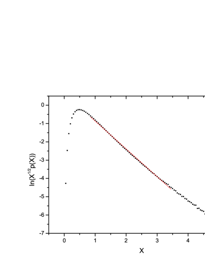
Figure 3: Fitting the distribution function of $X$ with $p(X)=CX^{-1/2}e^{-\beta X}(X\geq 1)$, where $X>1/\lambda^{2}$ implies NPT width is larger than $1$.

Now we calculate the average width of the NPT region. The probability for $N_{p}=1$ is given by

$$P_{1}=1-\int_{1/\lambda^{2}}^{+\infty}p(X)dX.$$ (29)

Neglecting the small possibility for $N_{p}>2$ at small $\lambda$, the probability of $N_{p}=2$, denoted by $P_{2}$, is given by $P_{2}=1-P_{1}$. Then, we have

$$\langle N_{p}\rangle=1+\int_{1/\lambda^{2}}^{+\infty}p(X)dX.$$ (30)

Completing the integration, for $\lambda\lesssim 1$, we obtain

$$\langle N_{p}\rangle=1+C\sqrt{\frac{\pi}{\beta}}\rm{erfc}(\sqrt{\frac{\beta}{\lambda^{2}}}),$$ (31)

where

$$\textmd{erfc}(x)=1-\frac{2}{\sqrt{\pi}}\int_{0}^{x}e^{-t^{2}}dt$$ (32)

is the complementary error function.

III.2 NPT width for $b=1$ at large $\lambda$

Next, we move to the case of large $\lambda$, in which $N_{p}$ is large. Still, for a given value of $\lambda$, due to the random nature of the off-diagonal elements of the Hamiltonian, $N_{p}$ has different values under different realizations of the off-diagonal elements. Thus, we need to study the probabilities for $N_{p}$ to take different values.

As discussed above, the value of $N_{p}$ is determined by properties of $s(U)$, and the matrix $U$ is split into an upper part $U_{\rm{up}}$ and a lower part $U_{\rm{down}}$. Thus, $s(U)=max\{s(U_{\rm{up}}),s(U_{\rm{down}})\}$. For $N$ large and $E_{\alpha}$ in the middle energy region, since the two sub-matrices have similar structure, we can consider one of them only, say, $s(U_{\rm{up}})$. For brevity, we use $s(U)$ to indicate this sub-matrix. For large $\lambda$, one has $p_{2}-E_{\alpha}\simeq E_{\alpha}-p_{1}\simeq N_{p}/2$.

Let us study the probability of $s(U)<1$ for a given value of $N_{p}$. For later convenience, we write this probability as $1-P(N_{p})$. Because the NPT width corresponds to the minimum value of $N_{p}$, for which $s(U)<1$, the probability that NPT width is $n$ is $(1-P(n))-(1-P(n-1))=P(n-1)-P(n)$. Then,

$$\langle N_{p}\rangle = \sum_{n=1}^{\infty}n(P(n-1)-P(n))$$ (33)

$$= \sum_{n=1}^{\infty}P(n)-\lim_{n\rightarrow\infty}nP(n).$$

Next we derive an approximate expression for $P(n)$. For this purpose, let us first estimate $s(U)$. Consider a series of $m-$dimensional sub-matrices truncated from $U$, denoted by $M_{i},i=0,1,2,\cdots,n$. An illustration of our truncation method is given in Fig.4. In the case of $b=1$, we take $m=5$. Generally, we require that $b<m\ll\lambda<N$.

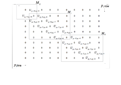
Figure 4: A series of matrices truncated from $U$ to estimate the maximum modulus of eigenvalues of $U$.

Specifically, sub-matrix $M_{i}$ is obtained by truncating $U$ from its $l_{i}$-th row to its $l_{i+1}$-th row, and from its $l_{i}$-th column to its $l_{i+1}$-th column, where $l_{i}=p_{1}-(m-1)i-1$. Elements of $M_{i}$ are given by

$$M_{i,pq}=U_{l_{i+1}+p-1,l_{i+1}+q-1}.$$ (34)

Thus, the sub-matrices ${M_{i}}$ contain all nonvanishing elements of $U$, and they are independent of each other. We found that $|s(U)-\max_{0\leq i\leq n}s(M_{i})|$ are not large (see Fig.5), hence, use the following approximation,

$$s(U)\approx\max_{0\leq i\leq n}s(M_{i}).$$ (35)

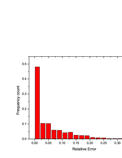
Figure 5: Error distribution of estimation in Eq.(35)

In the nonzero elements of $U$, the factors $1/(E_{\alpha}-E^{0}_{i})$ can be regarded as a constant for each $M_{i}$. Indeed, in the case of $i<p_{1}$ and $|i-j|<m\ll N_{p}$, one has

$$\left|\frac{1}{E_{\alpha}-E^{0}_{i}}-\frac{1}{E_{\alpha}-E_{j}}\right|\approx\frac{m}{(E_{\alpha}-E^{0}_{i})^{2}}\approx\frac{m}{N^{2}_{p}},$$ (36)

Introducing $a_{i}=E_{\alpha}-E_{p_{1}}+(m-1)i+1$ and noting Eq.(36), it is seen that the matrices $M$=$a_{i}M_{i}/\lambda$ can be regarded as realizations of the same independent random variables, independent of the label $i$. We call $M$ the standard $m$-dimensional matrix. It is easy to verify that $M$ is approximately a hermitian matrix and that its elements in upper triangle are

$$M_{ij}\approx v_{i}\delta_{i,j-1}\ (i\leq j),$$ (37)

where $v_{i}$ are independent, normally-distributed random variables with mean $0$ and variance $1$.

We use $h(x)$ to denote the distribution function of $s(M)$, and $H(x)$ for the corresponding cumulative distribution function, with $H(x)=\int_{0}^{x}h(x^{\prime})dx^{\prime}$. For brevity, we use $s_{M}$ to denote $s(M)$. According to definition of $M$, $M_{i}=\lambda M/a_{i}$, then $s(M_{i})=\lambda s_{M}/a_{i}$. Then making use of Eq.(35), we obtain

$$s(U)=\max_{0\leq i\leq n}(\lambda s_{M}/a_{i}).$$ (38)

We denote the distribution function of $s(U)$ by $w(s)$ and the corresponding cumulative distribution function by $W(s)$. Using Eq.(38), we obtain

$$W(s)=\prod_{i=0}^{n}H(\frac{a_{i}s}{\lambda}).$$ (39)

Let us first take logarithm for both sides of Eq.(39), then, approximate the summation on the right hand side by integration and obtain

$$\ln W(s)\approx\frac{\lambda}{m-1}\int_{a_{0}/\lambda}^{+\infty}\ln H(ts)dt,$$ (40)

where the upper limit is set $+\infty$ because we can regard the matrix as sufficient large. Note that $a_{0}\approx N_{p}/2$, thus we obtain from Eq.(40) that the probability of $s(U)<1$ is given by

$$\exp\left(\frac{\lambda}{m-1}\int_{N_{p}/2\lambda}^{+\infty}\ln H(t)dt\right).$$ (41)

Then,

$$P(n)=1-\exp\left(\frac{\lambda}{m-1}\int_{n/2\lambda}^{+\infty}\ln H(t)dt\right).$$ (42)

For $n\ll\lambda$, we have $P(n)\approx 1$. For $n$ increasing beyond $\lambda$, $P(n)$ decreases and approaches $0$.

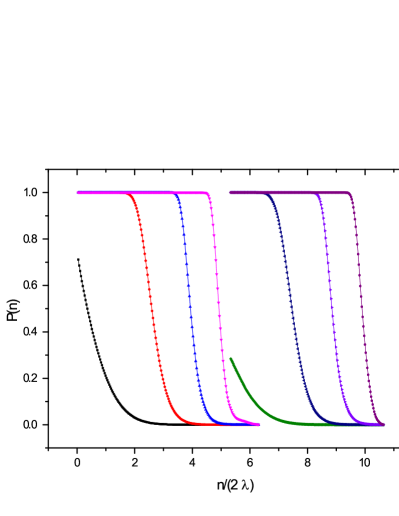
Figure 6: Curves of $P(n)$ as $b$ and $\lambda$ vary. We see that when $\lambda$ us sufficiently large, the curve is like heaviside for both $b$.

To evaluate the right hand of Eq.(42), we need to make use of our numerical results of $h(t)$ (see Appendix A). As shown in Fig.6, $P(n)$, as a function of $n/2\lambda$, has a ”ladder” shape when $\lambda$ is very large, and $nP(n)\rightarrow 0$ as $n\rightarrow\infty$. Then, from Eq.(33) and Eq.(42), we have

$$\langle N_{p}\rangle=n_{c},$$ (43)

where $n_{c}$ is the point at which $P(n_{c})=1/2$. Using Eq.(42), we obtain

$$\int_{n_{c}/2\lambda}^{+\infty}\ln H(t)dt=-\frac{(m-1)\ln 2}{\lambda}.$$ (44)

As $\lambda$ is large, the absolute value of the right side of Eq.(44) is small, hence, $n_{c}$ should be large. Discussions given in Appendix A show that

$$\int_{x}^{+\infty}\ln H(t)dt\sim-\frac{e^{-ax^{2}}}{x^{2}}(x\rightarrow+\infty).$$ (45)

Then, we get

$$\langle N_{p}\rangle\simeq C^{\prime}\lambda\sqrt{\ln\lambda}(\lambda\gg 1).$$ (46)

When $\lambda$ is not extremely large, one has $\langle N_{p}\rangle\propto\lambda$.

III.3 NPT width of Wigner-band random matrix:band width $b\geq 2$

In this section, we argue that Eq.(31) and Eq.(46) are still valid for $b\geq 2$, with coefficients in the equations as fitting parameters.

Let us first discuss the case of small $\lambda$. Here, we take the two matrices $U_{\rm{up}}$ and $U_{\rm{down}}$ [cf.Eqs.(13) and (14)] as the two $5b$-dimensional matrices nearest to $E_{\alpha}$. Neglecting terms of the order of $O(\lambda^{2})$ and higher in the eigen-equation, we obtain a condition similar to Eq.(23). Neglecting $B$ in the eigen-equation, the condition for $N_{p}=1$ is given by $A>1$. Writing $X=A/\lambda^{2}$, we use $p(X)=CX^{-1/2}e^{-\beta X}$ to fit the distribution of $X$. Finally, we also get Eq.(31), with $C$ and $\beta$ as fitting parameters.

Next, for large $\lambda$, when deriving Eq.(46), we need to use properties of $H(t)$ and the cumulative distribution function of the maximal eigenvalue of a standard $m$-dimensional random matrix. We can choose $m$, such that it is sufficiently larger than $b$ but still sufficiently smaller than $\lambda$. Then, the asymptotic behavior of $H(t)$ is still given by Eq.(45) (see Appendix A). Finally, the result Eq.(46) remains unchanged, with a different parameter $C^{\prime}$.

IV Numeral Results

In this section, we discuss our numerical results, including numerical tests of the analytical predictions given in the preceding section.

IV.1 Iterative algorithm for computing the width of NPT regions

In this subsection, we given an algorithm for computing NPT regions in the WBRM model. Its justification is given in Appendix. The algorithm consists of the following five steps.

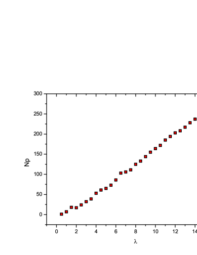
Figure 7: Confirmation of the new algorithm. For each perturbation strength $\lambda$, we randomly choose one Wigner band random matrix with $b=15$. Black squares represent NPT width calculated with ordinary method, and red circles represent NPT width calculated with our new iterative algorithm. Their consistency indicates that our algorithm is correct.

Step 1: Separate the matrix $H_{0}$ and $V$ into blocks as

$$H_{0}=\left(\begin{array}[]{cc}H_{0p}&0\\ 0&H_{0n}\end{array}\right),V=\left(\begin{array}[]{cc}V_{p}&*\\ &V_{n}\end{array}\right),$$ (47)

in which $p$ and $n$ stand for up and down. $H_{0p}$ and $V_{p}$ are both $[E_{\alpha}]\times[E_{\alpha}]$ square matrices, and $H_{0n}$ and $V_{n}$ are $N-[E_{\alpha}]$ dimensional square matrices. This option ensures that $E_{\alpha}-H_{0p}$ is positive definite and $E_{\alpha}-H_{0n}$ is negative definite.

Step 2: Compute $S_{p}$ and $S_{n}$,

$$S_{p}=\frac{1}{\sqrt{E_{\alpha}-H_{0p}}}\lambda V_{p}\frac{1}{\sqrt{E_{\alpha}-H_{0p}}},$$ (48)

$$S_{n}=\frac{1}{\sqrt{-(E_{\alpha}-H_{0n})}}\lambda V_{n}\frac{1}{\sqrt{-(E_{\alpha}-H_{0n})}}.$$ (49)

Step 3: Compute $I+S_{p}$, where $I$ is the identity matrix. Use Guassian elimination method to eliminate elements in the lower triangle part of $I+S_{p}$. In doing this, when all the lower-triangle elements in the $i$th column are eliminated, a diagonal element $y_{i+1}$ is gained in the $(i+1)$-th row and column. We terminate the procedure when a diagonal element $y_{i_{c1}}<0$ is obtained.

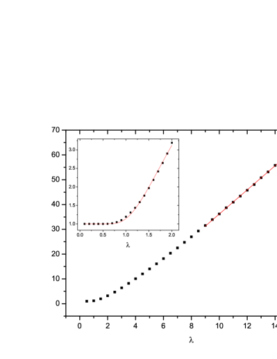
Figure 8: Average NPT width towards perturbation strength $\lambda$ for Wigner-band random matrices with band width $b=1$. When $\lambda$ is small, we fit the scatters with Eq.(31). When $\lambda$ is relatively large, we fit linear.

Step 4: Apply the same procedure as in step 3 to $I-S_{p}$ and obtain a $y_{i_{c2}}<0$. Then, $p_{1}=max\{i_{c1},i_{c2}\}$.

Step 5: For $I+S_{n}$ and $I-S_{n}$, we eliminate the elements in the upper triangle by the Gaussian-elimination method starting from the last line. Similar to steps 3 and 4, we take $p_{2}$ as the smaller $i_{c}$ obtained from the two matrices. The NPT width is then given by $N_{p}=p_{2}-p_{1}$.

The algorithm discussed above is applicable only for the case where $p_{2}-p_{1}>b$, in which the elements in $*$ of $V$ do not take part in the elimination. Practically, for a given band matrix, we first apply the above-discussed iterative algorithm to compute $p_{2}$ and $p_{1}$. If $N_{p}=p_{2}-p_{1}\leq b$, then, we turn to the ordinary method to compute $N_{p}$.

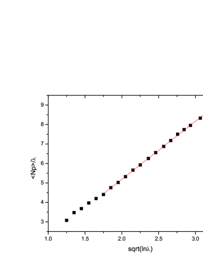
Figure 9: Average NPT width towards perturbation strength $\lambda$ for Wigner band random matrices with band width $b=1$ when $\lambda$ is very large. We change the axis to make a linear fit with Eq.(46).

Finally, we discuss efficiency of the above-discussed algorithm. Similar to the method of Gaussian elimination, the algorithm has a time complexity $O(Nb^{2})$. Furthermore, the elimination is from top and bottom to the middle of the matrix. Thus, when $\lambda$ is relatively large and $p_{1}$ and $p_{2}$ are far away from middle, we do not need to eliminate the total $N$ lines to find $p_{1}$ and $p_{2}$. We remark that our algorithm is particularly useful for large $\lambda$. For small $\lambda$ and not large $b$, $N_{p}<b$ and the ordinary method of computing $N_{p}$ is not quite time-consuming. Detailed discussions of the algorithm is given in Appendix B and C.

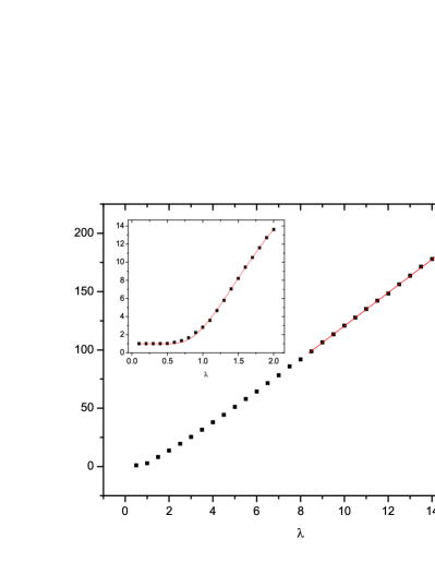
Figure 10: Average NPT width towards perturbation strength $\lambda$ for Wigner band random matrices with band width $b=8$. When $\lambda$ is small, we fit the scatters with Eq.(31). When $\lambda$ is relatively large, we fit linear.

We have numerically tested the validity of the above-discussed algorithm (see Fig.7).

IV.2 Variation of the NPT width with perturbation strength

According the analytical study discussed in Sec.III, for $b=1$, we have the following picture for variation of $\langle N_{p}\rangle$, the average width of the NPT regions of EFs. That is, in the perturbation regime from weak to somewhat medium, specifically, for $\lambda\lesssim 1$, it follows Eq.(31). One should note that, since the level spacing of the unperturbed Hamiltonian is one, the perturbation is not weak at $\lambda=1$. While, for large $\lambda$, the behavior is given by Eq.(46). For $\lambda$ not very large, Eq.(46) shows that the width increases almost linearly with $\lambda$, but, effect of the logarithm term should be seen for sufficiently large $\lambda$.

As shown in Fig.8, Eq.(31) works quite well for $\lambda$ below $2$. For $\lambda$ beyond $9$, $N_{p}$ has a good linear behavior in agreement with the prediction of Eq.(46) for $\lambda$ not very large. For very large $\lambda$, the contribution of $\sqrt{\ln\lambda}$ in Eq.(46) becomes unnegligible, as shown in Fig.9.

We further increase the width $b$ of the Hamiltonian matrices. As shown in Fig.10, our predictions also works well in this case. For $b>1$, the parameters $C$ and $\beta$ in Eq.(31) and parameter $C^{\prime}$ in Eq.(46) are fitting parameters.

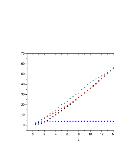
Figure 11: Average NPT width(black squares), LDOS halfwidth(dark green triangles), half width of eigenstates(red circles) and localization length(blue triangles) for Wigner band random matrices with band width $b=1$.

IV.3 NPT width and half-width of LDOS

As discussed previously, the half-width of LDOS should be closely related to the width of NPT regions of EFs [cf.Eq.(19)]. In this subsection, we numerically test this prediction.

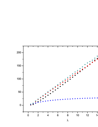
Figure 12: Average NPT width(black squares), LDOS halfwidth(dark green triangles), half width of eigenstates(red circles) and localization length(blue triangles) for Wigner band random matrices with band width $b=8$.

In Fig.11, Fig.12, and Fig.13, we give variation of $N_{p}$, $w_{L}$, and $w_{F}$ with the perturbation strength $\lambda$. We also plot the average of the localization length $L_{\alpha}$, denoted by $L$, where

$$L_{\alpha}=1/\sum_{j}|C_{\alpha j}|^{4}.$$ (50)

At large $\lambda$, both $w_{L}$ and $w_{EF}$ are much larger than $L$, which is a phenomenon called localization in the energy shell.

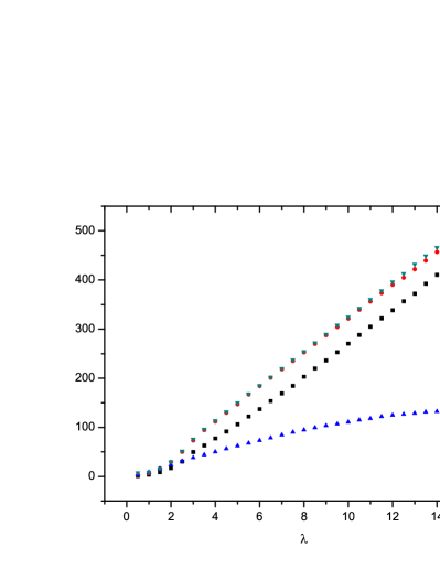
Figure 13: Average NPT width(black squares), LDOS halfwidth(dark green triangles), half width of eigenstates(red circles) and localization length(blue triangles) for Wigner band random matrices with band width $b=50$.

Finally, we discuss Eq.(19). We plot $\eta$ versus $\lambda$ in Fig.14. It is seen that $\eta\approx 1$ in the middle region of $\lambda$, and is small in the weak or strong perturbation regimes.

Figure 14: Value of $\eta$ against $\lambda$ for $b=8$, $N=500$. $\eta\approx 1$ for middle-strength perturbation, and is small in weak or strong perturbation.

V Conclusions

In this paper, we have studied the NPT and PT parts of EFs in the WBRM model. It is shown that the width of the LDOS can be estimated, if the width of NPT regions of EFs are known. For $b=1$, we have derived explicit expressions for the average width of NPT regions, as functions of the perturbation strength $\lambda$, for $\lambda\gtrsim 1$ and for large $\lambda$. Numerically, we have found that these expressions are still valid for $b>1$. We have also developed a algorithm, which can efficiently compute the width of NPT regions at large $\lambda$, with a time complexity less than $O(b^{2}N)$.

Appendix A asymptotic property of $H(t)$ and properties of $P(n)$

Previously, we define $h(t)$ as the distribution function of the maximal modulus of eigenvalues of a standard $m$-dimensional random matrix $M_{s}$, whose elements take the form

$$M_{s,ij}=\left\{\begin{array}[]{cc}v_{ij}\sim N(0,1),&1\leq|i-j|\leq b\\ 0,&\rm{others}.\end{array}\right.$$ (51)

and a corresponding cumulative distribution function $H(t)$. We now explicitly show the curves of $h(t)$ when $b=1$ and $b=8$ obtained by a Monte Carlo simulation in Fig.15 and Fig.16. We fit the region of large $t$ by Guassian formula and show the asymptotic property of $h(t)$ that

$$h(t)\sim e^{-t^{2}}(t\rightarrow\infty).$$ (52)

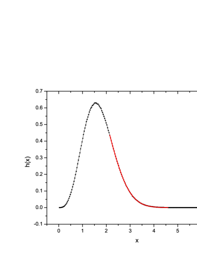
Figure 15: Density function $h(x)$ of the maximum absolute value of eigenvalues of a standard random matrix with $b=1$. Guassian fit of the large-$\lambda$ region is shown in red curve.

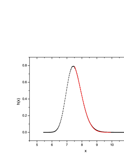
Figure 16: Density function $h(x)$ of the maximum absolute value of eigenvalues of a standard random matrix with $b=8$. Guassian fit of the large-$\lambda$ region is shown in red curve.

Making use of

$$H(x)=1-\int_{x}^{+\infty}h(t)dt$$ (53)

and

$$\int_{x}^{+\infty}t^{-n}e^{-t^{2}}dt\sim x^{-n-1}e^{-x^{2}},$$ (54)

we obtain

$$1-H(t)\sim\frac{e^{-t^{2}}}{t}(t\rightarrow\infty).$$ (55)

We take first order approximation that $\ln(1-H(t))\approx-H(t)$ and use Eq.(54) to obtain

$$\int_{x}^{+\infty}\ln H(t)dt\sim\frac{e^{-x^{2}}}{x^{2}},$$ (56)

which is just Eq.(45).

Appendix B Verification of the iterative algorithm

To develop our algorithm, we first make a similarity transformation to $U$ to create a symmetrical matrix. We first consider the upper part of $U$ called $U_{p}$ ,for $Q$ naturally split $U$ into two independent parts. We will denote the correspondingly upper part of $V$ and $H_{0}$ as $V_{p}$ and $H_{0p}$. Note that $Q$ and $1/(E_{\alpha}-H_{0})$ commute, so we rearrange $U^{n}_{p}$ as

$$U^{n}_{p}=Q\frac{1}{\sqrt{E_{\alpha}-H_{0p}}}S_{p}^{n-1}\frac{1}{\sqrt{E_{\alpha}-H_{0p}}}\lambda Q,$$ (57)

where

$$S_{p}=\frac{1}{\sqrt{E_{\alpha}-H_{0p}}}\lambda V_{p}\frac{1}{\sqrt{E_{\alpha}-H_{0p}}}.$$ (58)

Then the condition $s(U_{p})<1$ is equivalent to $s(S_{p})<1$, with $S_{p}$ obviously symmetrical and with the same band width.

Now we recall some results in linear algebra.GBW A real symmetrical matrix has real eigenvalues, and condition $s(S_{p})<1$ is equivalent to $I\pm S_{p}$ are both positive definite, where $I$ is the identity matrix. The sufficient and necessary condition for a symmetrical matrix to be positive definite is that its ordered main subdeterminants(denoted by $d_{i}$) are all positive. We will calculate the ordered main subdeterminants of $I\pm S_{p}$ by elementary row transformations. To be clear, we first deal with the case where $b=1$.

In this simpler case, one can prove that if $S_{p}$ has a positive eigenvalue $x_{0}$, it must have a corresponding eigenvalue $-x_{0}$, so we only need to verify the condition under which $I+S_{p}$ is positive definite. Recall the elementary row transformation matrices $T_{ij}(\mu)$, with all diagonal elements $1$ and only nonvanishing element $\mu$ in the $i$th column and $t$th row, and multiplying $T_{ij}(\mu)$ from the left gives an elementary row transformation that does not change any its subdeterminant. Suppose the elements of $S_{p}$ take the form

$$S_{p}(i,i+1)=S_{p}(i+1,i)=\xi_{i}(i=1,2,\cdots,p_{1}-2),$$ (59)

then $d_{1}=1$, and we can continuously multiply $T_{i,i+1}(\mu_{i})$ from the left to eliminate the element of $I+S_{p}$ in lower triangle to obtain $d_{i+1}$. For instance, our first step is that

$$T_{12}(-\xi_{1})(I+S_{p})=\left(\begin{array}[]{ccccc}1&&&&\\ -\xi_{1}&1&&&\\ &&1&&\\ &&&\ddots&\\ &&&&1\end{array}\right)\left(\begin{array}[]{ccccc}1&\xi_{1}&&&\\ \xi_{1}&1&\xi_{2}&&\\ &\xi_{2}&1&&\\ &&&\ddots&\xi_{p_{1}-2}\\ &&&\xi_{p_{1}-2}&1\end{array}\right)=\left(\begin{array}[]{ccccc}1&\xi_{1}&&&\\ 0&1-\xi^{2}_{1}&\xi_{2}&&\\ &\xi_{2}&1&&\\ &&&\ddots&\xi_{p_{1}-2}\\ &&&\xi_{p_{1}-2}&1\end{array}\right),$$ (60)

so $\mu_{1}=-\xi_{1}$, and $d_{2}=1-\xi^{2}_{1}$. If $d_{2}>0$, then we multiply $T_{23}(-\xi_{2}/(1-\xi^{2}_{1}))$ from the left to obtain $d_{3}$. Now we introduce the sequence $\{y_{i}\}$ to denote the new diagonal element before $i$th elimination, then $y_{1}=1,y_{2}=d_{2}/d_{1}=1-\xi^{2}_{1},\cdots,y_{i}=d_{i}/d_{i-1},\cdots$. We can construct a recursive formula for $y_{i+1}$ by the $i$th elimination

$$T_{i,i+1}(-\frac{\xi_{i+1}}{y_{i}})\left(\begin{array}[]{cccccccc}y_{1}&\xi_{1}&&&&&&\\ &y_{2}&\xi_{2}&&&&&\\ &&\ddots&\ddots&&&&\\ &&&y_{i}&\xi_{i}&&&\\ &&&\xi_{i}&1&\xi_{i+1}&&\\ &&&&\xi_{i+1}&1&&\\ &&&&&&\ddots&\xi_{p_{1}-2}\\ &&&&&&\xi_{p_{1}-2}&1\end{array}\right)=\left(\begin{array}[]{cccccccc}y_{1}&\xi_{1}&&&&&&\\ &y_{2}&\xi_{2}&&&&&\\ &&\ddots&\ddots&&&&\\ &&&y_{i}&\xi_{i}&&&\\ &&&0&y_{i+1}&\xi_{i+1}&&\\ &&&&\xi_{i+1}&1&&\\ &&&&&&\ddots&\xi_{p_{1}-2}\\ &&&&&&\xi_{p_{1}-2}&1\end{array}\right),$$ (61)

from which we obtain

$$y_{i+1}=1-\frac{\xi^{2}_{i}}{y_{i}}(i\geq 1);y_{1}=1.$$ (62)

Finally we obtain our algorithm to calculate $p_{1}$ for the case $b=1$. As $p_{1}$ is the maximal row number that ensures all ordered main subdeterminants $d_{i}$ of $I+S_{p}$ positive, we require that $\forall i\leq p_{1}-1,y_{i}>0$. Given a matrix $S$, we continuously apply Eq.(62), until we obtain a $y_{i_{c}}<0$, then $p_{1}=i_{c}$. Similarly, if we set $y_{N}=1$, we can obtain $p_{2}$ by adopting the same recursive formula for $y_{i-1}$, then obtain $N_{p}=p_{2}-p_{1}$. We can also verify this algorithm by path summation in Appendix C. Now we expand our algorithm to the cases where $b\geq 2$. In this case, our way above to calculate ordered subdeterminants $d_{i}$ is still applicable. Every time we eliminate elements in a column in lower triangle of $I\pm S_{p}$ by elementary row transformations $b$ times, we obtain a higher ordered subdeterminant. We end the iteration until we find a negative $i_{c}$-order subdeterminant. Only difference lies in that we need to both compute $i_{c}$ for $I\pm S_{p}$, and choose $p_{1}$ as the smaller one.

Similarly, we can use the algorithm calculate $p_{2}$, then we obtain the NPT width $N_{p}=p_{2}-p_{1}$.

Appendix C path summation derivation for the iterative algorithm

We provide a new picture for our recursive formula Eq.(62). Recall that NPT width is the minimal dimension of subspace $P$ such that the generalized Brillouin-Wigner perturbation expansion Eq.(6) converges. Decompose $|\alpha_{s}\rangle$ as summation of NPT eigenstates,

$$|\alpha_{s}\rangle=\sum_{i=p_{1}}^{p_{2}}t_{i}|i\rangle,$$ (63)

then convergence of Eq.(6) is equivalent to convergence of

$$C_{ij}=\langle j|i\rangle+\sum_{m=1}^{n-1}\langle j|T^{m-1}|i\rangle+\langle j|T^{n}|i\rangle+\cdots$$ (64)

for any $i\in[p_{1},p_{2}]$, and any $j$. Note that the definition of $T$ (Eq.(5)) consists of a projection operator $Q$, so we only need to check the convergence of Eq.(64) for the case where $j\notin[p_{1},p_{2}]$. Using Eq.(5) and Eq.(64), we can write the explicit formula for $C_{ij}$,

$$C_{ij}=\frac{\lambda V_{ji}}{E_{\alpha}-E_{j}}+\sum_{k_{1}\in Q}\frac{\lambda V_{jk_{1}}}{E_{\alpha}-E_{j}}\frac{\lambda V_{k_{1}i}}{E_{\alpha}-E_{k_{1}}}$$

$$+\sum_{k_{1},k_{2}\in Q}\frac{\lambda V_{jk_{1}}}{E_{\alpha}-E_{j}}\frac{\lambda V_{k_{1}k_{2}}}{E_{\alpha}-E_{k_{1}}}\frac{\lambda V_{k_{2}i}}{E_{\alpha}-E_{k_{2}}}+\cdots.$$ (65)

By definition of NPT width, we need to find the maximal dimension of $Q$ such that Eq.(C) converges. For simplicity, we only consider the case where $b=1$. Let we call the chain $k_{0}=j\rightarrow k_{1}\rightarrow\cdots\rightarrow k_{n}\rightarrow i=k_{n+1}$ a $(n+1)$-order path, then the $n$th term in Eq.(C) is a summation over all $n$-order paths. We denote $\lambda V_{{k_{i}}{k_{i+1}}}/(E_{\alpha}-E_{k_{i}})$ as $f(k_{i}\rightarrow k_{i+1})$, then, as $b=1$, it vanishes unless $|k_{i+1}-k_{i}|=1$.

For $b=1$, $Q$ subspace is naturally split into to two separate parts,$[1,p_{1}-1]$ and $[p_{2}+1,N]$. Then the summation Eq.(C) vanishes unless $i=p_{1}$ or $i=p_{2}$, where the summation only covers paths in one side of $Q$ subspace. Two sides of $Q$ subspaces are similar, so let us consider the case where $i=p_{1}$. We claim that convergence of Eq.(C) for $j=p_{1}-1$ implies convergence for any $j\in[1,p_{1}-2]$. This is because if for one of $j\in[1,p_{1}-2]$ the path summation Eq.(C) diverges, then for any path $j\rightarrow\cdots\rightarrow i$, we can construct a path $j+1\rightarrow j\rightarrow\cdots\rightarrow i$, and summation over all these paths also diverges because it is just $f(j+1\rightarrow j)$ times the former summation, meaning that $C_{{p_{1}}{j+1}}$ also diverges. Iterate the reasoning above leads to contradiction to our condition that $C_{{p_{1}}{p_{1}-1}}$ converges. Therefore later we only consider the case where $i=p_{1}$ and $j=p_{1}-1$.

Since the only way to $p_{1}$ is through $p_{1}-1$, We rewrite Eq.(C) as

$$C_{{p_{1}}{p_{1}-1}}=f(p_{1}-1\rightarrow p_{1})A(p_{1}-1\rightarrow p_{1}-1),$$ (66)

where $A(j\rightarrow j)$ represents the path summation over paths starting at $j$ and ending at $j$, without passing through $j+1$. Now we classify the paths from $p_{1}-1$ to $p_{1}-1$ by the number of times the path includes $p_{1}-1$ in the middle. Suppose all paths(excluded the beginning) that include $p_{1}-1$ one time contribute $g(p_{1}-1)$ to the path summation, then all paths that include $p_{1}-1$ $n$ times contribute $g^{n}(p_{1}-1)$. Then

$$A(p_{1}-1\rightarrow p_{1}-1) = \sum_{n=1}^{\infty}g^{n}(p_{1}-1)$$ (67)

$$= \frac{1}{1-g(p_{1}-1)}-1,$$

which converges only when $|g(p_{1}-1)|<1$. Next we consider the paths that contribute to $g(p_{1}-1)$. We may first go to $p_{1}-2$, then return to $p_{1}-1$, then the path contributes $f(p_{1}-1\rightarrow p_{1}-2)f(p_{1}-2\rightarrow p_{1}-1)$ to the summation. By definition, all paths that goes to $p_{1}-2$ then returns to $p_{1}-2$ contributes to a factor $A(p_{1}-2\rightarrow p_{1}-2)$, then

$$g(p_{1}-1) = f(p_{1}-1\rightarrow p_{1}-2)f(p_{1}-2\rightarrow p_{1}-1)$$ (68)

$$\times (1+A(p_{1}-2\rightarrow p_{1}-2)).$$

Using Eqs.(67), (68), we obtain

$$g(p_{1}-1) = f(p_{1}-1\rightarrow p_{1}-2)f(p_{1}-2\rightarrow p_{1}-1)$$ (69)

$$\times \frac{1}{1-g(p_{1}-2)}.$$

The reasoning above applies to any $j\in[1,p_{1}-1]$. Note that $g(1)=0$ by definition, then we obtain the recursive formula

$$g(j+1)=f(j+1\rightarrow j)f(j\rightarrow j+1)\frac{1}{1-g(j)};g(1)=0.$$ (70)

Direct calculation of matrix elements shows that

$$f(j+1\rightarrow j)f(j\rightarrow j+1)=\xi^{2}_{j},$$ (71)

in which $\xi^{2}_{j}$ shares the same meaning with that in Eq.(40). Now let $y_{i}=1-g(i)$, then Eq.(B8) becomes

$$y_{i+1}=1-\frac{\xi^{2}_{i}}{y_{i}};y_{1}=1,$$ (72)

which is exactly Eq.(62).

In this approach, path summation converges if and only if $g(p_{1}-1)<1$, i.e, $y_{p_{1}-1}>0$. Therefore, as we proceed our iteration, if we find a $y_{i_{c}}<0$, then $i_{c}=p_{1}$, which is consistent with our previous derivation by elementary row transformation. $p_{2}$ can be derived by similar approach.

References

- (1) B.Lauritzen, et al., Phys. Rev. Lett. 74, 5190 (1995).
- (2) Ph. Jacquod, D.L. Shepelyansky, O. P. Sushkov, Phys. Rev. Lett. 78, 923 (1997)
- (3) Carlos Mejia-Monasterio, et al., Phys. Rev. Letts. 81, 5189 (1998)
- (4) V.V.Flambaum and F. M. Izrailev, Phys. Rev. E 61, 2539(2000); ibid., 64, 026124 (2001)
- (5) P. R. Zangara, et al., Phys. Rev. A 86, 012322 (2012).
- (6) Lea F. Santos, F.Borgonovi and F.M. Izrailev, Phys. Rev. Lett. 108, 094102 (2012).
- (7) E. J. Torres-Herrera and Lea F. Santos, Phys. Rev. A 89, 043620 (2014); ibid., 90, 033623 (2014).
- (8) Wen-ge Wang, Phys. Rev. E 61, 952 (2000); ibid. 65, 036219 (2002).
- (9) G. Casati, B.V. Chirikov, I. Guarneri, and F.M. Izrailev, Phys.Lett.A 223, 430 1996.
- (10) W.-G. Wang, F.M. Izrailev, and G. Casati, Phys. Rev. E 57, 323 (1998).
- (11) W.-g. Wang, Phys. Rev. E 61, 952 (2000).
- (12) E. Wigner, Ann. Math. 62, 548 (1955); 65, 203 (1957).