Nonperturbative Renormalization in the RI-SMOM Scheme and Gribov Uncertainty in the RI-MOM Scheme for Staggered Bilinears

Abstract:

We present results of renormalization factors for bilinear operators obtained using the nonperturbative renormalization method (NPR) in the RI-SMOM schemes. The operators are constructed using HYP staggered quarks on the MILC asqtad lattice ($N_{f}=2+1$). We compare results in the RI-SMOM schemes with those in the RI-MOM scheme for the $V\otimes S$ and $S\otimes S$ operators. Since we use Landau gauge fixing, we study the effect of Gribov ambiguity on the wave function renormalization $Z_{q}$ in the RI-MOM scheme. We find that the Gribov uncertainty is negligibly small for $Z_{q}$ in the RI-MOM scheme.

1 Introduction

In Ref. [1], the SWME collaboration reported that there exists 3.4$\sigma$ tension in $\varepsilon_{K}$ (indirect CP violation parameter in neutral kaons) between the experiment and the theoretical evaluation directly from the standard model (SM) with the lattice QCD inputs. In order to determine $\varepsilon_{K}$ theoretically, we need to know the kaon bag parameters such as $B_{K}$ (in the SM) [2] and $B_{2-5}$ [3] (in the BSM). Here, we need to know the matching factors which convert lattice data for $B_{i}$ into the corresponding quantities defined in the ${\overline{\text{MS}}}$ scheme in the continuum. Here, we use the non-perturbative renormalization (NPR) method to determine the matching factors in the RI-SMOM scheme [4]. The results will be compared with those in the RI-MOM scheme [5]. We will also address Gribov ambiguity in NPR [6].

2 NPR of Staggered Bilinears in the RI-SMOM Scheme

A general staggered bilinear operator can be written as

$$O^{S\otimes F}_{i}(y) =\sum_{AB}\overline{\chi}_{i}(y_{A})\overline{(\gamma_{S}\otimes\xi_{F})}_{AB}U_{i;AB}(y)\chi_{i}(y_{B})$$ (1)

where $\overline{(\gamma_{S}\otimes\xi_{F})}_{AB}=\frac{1}{4}\textrm{tr}[\gamma_{A}^{\dagger}\gamma_{S}\gamma_{B}\gamma_{F}^{\dagger}]$ and $\gamma_{A}=\gamma_{1}^{A_{1}}\gamma_{2}^{A_{2}}\gamma_{3}^{A_{3}}\gamma_{4}^{A_{4}}$. The original coordinate is $y_{A}$ = $2y+A$ where $A,B$ are hypercube vectors (each element is 0 or 1). $y$ is the hypercube coordinate on the lattice with its spacing $2a$. $S$ and $F$ stand for the spin and taste degree, respectively. $i$ is the gauge configuration index and it will be averaged over gauge ensemble when we calculate the correlation function. $\chi$ and $\overline{\chi}$ are the staggered quark fields. Here, we use the HYP-blocked fat links for $U_{\mu}$.

We can obtain the amputated Green’s function $\widetilde{\Lambda}^{S\otimes F}_{c_{1}c_{2}}(\widetilde{p}_{1}+\pi_{A},\widetilde{p}_{2}+\pi_{B})$ for the bilinear operators by removing the external quark lines as in Ref. [5]. Here, we use the reduced momentum $\widetilde{p}_{1}\in(-\frac{\pi}{2a},\frac{\pi}{2a}]^{4}$ defined in the reduced Brillouin zone. For details, refer to Ref. [5].

We define the projected amputated Green’s function $\Gamma$ as

$$\Gamma^{\alpha\beta}(\widetilde{p}_{1},\widetilde{p}_{2})=\sum_{AB}\sum_{c_{1}c_{2}}[\widetilde{\Lambda}^{\alpha}_{c_{1}c_{2}}(\widetilde{p}_{1}+\pi_{A},\widetilde{p}_{2}+\pi_{B})\hat{\mathbb{P}}^{\beta}_{BA;c_{2}c_{1}}],\quad\hat{\mathbb{P}}^{\beta}_{BA;c_{2}c_{1}}=\frac{1}{48}\overline{\overline{(\gamma^{\dagger}_{S^{\prime}}\otimes\xi^{\dagger}_{F^{\prime}})}}_{BA}\delta_{c_{2}c_{1}}$$ (2)

where $\alpha=(\gamma_{S}\otimes\xi_{F})$, $\beta=(\gamma_{S^{\prime}}\otimes\xi_{F^{\prime}})$, and $\overline{\overline{(\gamma_{S}\otimes\xi_{F})}}_{AB}=\frac{1}{16}{\sum_{CD}}(-1)^{A\cdot C}\overline{(\gamma_{S}\otimes\xi_{F})}_{CD}(-1)^{D\cdot B}$.

2.1 RI-SMOM schemes

In the RI-SMOM renormalization scheme, we use symmetric momentum $\widetilde{p}_{1}^{2}=\widetilde{p}_{2}^{2}=\widetilde{q}^{2}$ at the subtraction momentum $\widetilde{q}\equiv\widetilde{p}_{1}-\widetilde{p}_{2}$. The subtraction scheme is that $\Gamma^{\alpha\beta}_{R}(\widetilde{p}_{1},\widetilde{p}_{2})=\delta_{\alpha\beta}$, where the sub-index $R$ represents the renormalized quantity. We define renormalization factors $Z$ by $\Gamma_{R}^{\alpha\sigma}=\sum_{\beta}Z_{q}^{-1}Z^{\alpha\beta}\Gamma^{\beta\sigma}_{B}$ where where the sub-index $B$ represents bare (=unrenormalized) quantity.

Let us consider the conserved vector current. There are three different projection methods available in this case [4]. The first choice is the $\textrm{RI-SMOM}_{\gamma_{\mu}}$ scheme in which the subtraction scheme is defined as

$$\Gamma^{V\otimes S}_{R}(\widetilde{p}_{1},\widetilde{p}_{2})|_{\text{smom}} \equiv\frac{1}{4}\sum_{\mu}\sum_{AB}\sum_{c_{1}c_{2}}[\widetilde{\Lambda}^{V_{\mu}\otimes S}_{c_{1}c_{2}}(\widetilde{p}_{1}+\pi_{A},\widetilde{p}_{2}+\pi_{B})\hat{\mathbb{P}}^{V_{\mu}\otimes S}_{BA;c_{2}c_{1}}]_{\text{smom}}=1\,.$$ (3)

The second choice is the RI-SMOM scheme in which the subtraction scheme is

$$\Gamma^{V\otimes S}_{R}(\widetilde{p}_{1},\widetilde{p}_{2})|_{\text{smom}} \equiv\frac{1}{\widetilde{q}^{2}}\sum_{\mu}\sum_{AB}\sum_{c_{1}c_{2}}[\widetilde{q}_{\mu}\widetilde{\Lambda}^{V_{\mu}\otimes S}_{c_{1}c_{2}}(\widetilde{p}_{1}+\pi_{A},\widetilde{p}_{2}+\pi_{B})\sum_{\nu}\widetilde{q}_{\nu}\hat{\mathbb{P}}^{V_{\nu}\otimes S}_{BA;c_{2}c_{1}}]_{\text{smom}}=1\,,$$ (4)

where $\widetilde{q}=\widetilde{p}_{1}-\widetilde{p}_{2}$. One advantage of this scheme is that its anomalous dimension for $Z_{q}$ is already known up to the 4-loop level [4]. The third choice is the RI-SMOM-sin scheme in which the subtraction scheme is defined as

$$\Gamma^{V\otimes S}_{R}(\widetilde{p}_{1},\widetilde{p}_{2})|_{\text{smom}} \equiv\frac{1}{\hat{q}^{2}}\sum_{\mu}\sum_{AB}\sum_{c_{1}c_{2}}[\hat{q}_{\mu}\widetilde{\Lambda}^{V_{\mu}\otimes S}_{c_{1}c_{2}}(\widetilde{p}_{1}+\pi_{A},\widetilde{p}_{2}+\pi_{B})\sum_{\nu}\hat{q}_{\nu}\hat{\mathbb{P}}^{V_{\nu}\otimes S}_{BA;c_{2}c_{1}}]_{\text{smom}}=1\,,$$ (5)

where $\hat{q}_{\mu}\equiv\sin(a\widetilde{q}_{\mu})$ and $\hat{q}^{2}=\sum_{\mu}\hat{q}_{\mu}^{2}$.

The conserved current does not receive any renormalization and so $Z_{V}=1$. Hence, $\Gamma^{V\otimes S}_{R}=Z_{q}^{-1}Z_{V}\Gamma_{B}^{V\otimes S}=1$ leads to $Z_{q}=\Gamma_{B}^{V\otimes S}$. Similarly, another Ward identity $Z_{S}\cdot Z_{m}=1$ leads to the identity $Z_{m}=\Gamma_{B}^{S\otimes S}/\Gamma_{B}^{V\otimes S}$. Here, note that the running of $Z_{m}$ is different between $\textrm{RI-SMOM}_{\gamma_{\mu}}$ and (RI-SMOM & RI-SMOM-sin) schemes [7].

2.2 Simulation Details

We use $N_{f}=2+1$, $20^{3}\times 64$ MILC asqtad ensembles ($a\approx 0.12fm$, $am_{\ell}/am_{s}=0.01/0.05$). Valence quarks are HYP-smeared staggered fermions with ($am_{q}=$ 0.01, 0.02, 0.03, 0.04, 0.05). We use 10 gluon configurations with Landau gauge fixing.

$n_{1}$	$n_{2}$	$(a\widetilde{p})^{2}$	$(a\widetilde{p})^{4}$	GeV
$(1,1,0,0)$	$(1,0,1,0)$	0.1974	0.0195	0.7363
$(2,2,0,0)$	$(2,0,2,0)$	0.7896	0.3117	1.4727
$(3,3,0,0)$	$(3,0,3,0)$	1.7765	1.5780	2.2090
$(4,4,0,0)$	$(4,0,4,0)$	3.1583	4.9873	2.9454
$(5,5,0,0)$	$(5,0,5,0)$	4.9348	12.1761	3.6817

(a) Simple momenta

$n_{1}$	$n_{2}$	$(a\widetilde{p})^{2}$	$(a\widetilde{p})^{4}$	GeV
$(1,2,3,0)$	$(-2,3,1,0)$	1.3817	0.9546	1.9482
$(2,4,2,0)$	$(-2,2,4,0)$	2.3687	2.8054	2.5508
$(1,3,4,0)$	$(-3,4,1,0)$	2.5661	3.2924	2.6549

(b) Complicated momenta

Table 1: List of symmetric momenta: $a\widetilde{p}_{\mu}\equiv\frac{2\pi}{L_{\mu}}n_{\mu}$ with $L_{S}^{3}\times L_{T}=20^{3}\times 64$. $\widetilde{p}^{2}=\displaystyle\sum_{\mu}\widetilde{p}_{\mu}^{2}$ and $\widetilde{p}^{4}=\displaystyle\sum_{\mu}\widetilde{p}_{\mu}^{4}$ .

We calculate $\Gamma_{B}^{\mathcal{O}}(m,\widetilde{p}^{2})$ with external quark momenta $\widetilde{p}$ listed in Table 1. First, we obtain $Z_{\mathcal{O}}$ at $\mu_{1}^{2}={\widetilde{q}}^{2}$. Second, we use the RG evolution from the scale $\mu_{1}$ to the common scale $\mu_{0}=3$ GeV. In the RG running, we use the anomalous dimension obtained using the perturbation theory as in Refs. [7, 8].

2.3 Chiral extrapolation

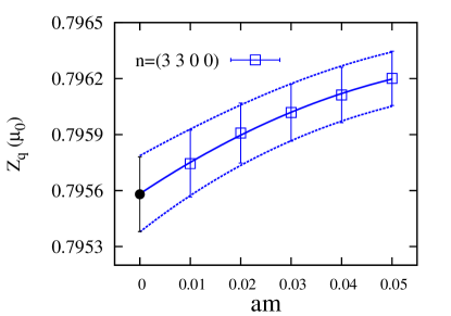
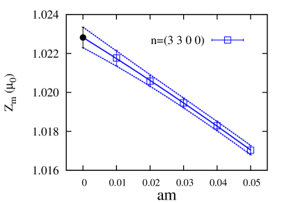
Figure 1: Chiral extrapolation of $Z_{q}$ in RI-SMOM scheme at $\mu_{0}=3$ GeV. Black circled points are the chiral limit data obtained from the fitting.

Here, we perform the chiral extrapolation for $Z_{q}$ and $Z_{m}$. In Fig. 1, we present results of chiral extrapolation in $Z_{q}$ and $Z_{m}$. The data in the plots are obtained at the common scale $\mu_{0}=3$ GeV with a momentum of (3,3,0,0) in the RI-SMOM scheme. Here, we use the quadratic fitting to obtain $Z_{q}$ and $Z_{m}$ in the chiral limit. The fitting results are summarized in Table 2.

	$c_{0}$	$c_{1}$	$c_{2}$	$\chi^{2}/\text{d.o.f}$
$Z_{q}$	0.79558(20)	0.0180(46)	-0.114(52)	0.0041(45)
$Z_{m}$	1.02282(53)	-0.107(18)	-0.18(20)	0.011(12)

Table 2: Fitting result of chiral extrapolation in the Fig. 1 where fitting the function is $c_{0}+c_{1}(am)+c_{2}(am)^{2}$.

2.4 Results: Momentum Fit for $Z_{q}$

Here, we explain the p-fit procedure for $Z_{q}$. In the case of $Z_{q}$, we have tried to fit the data of both simple and complicated momenta to fitting functional forms up to $\mathcal{O}((a\widetilde{p})^{6})$, and we have failed in finding a reliable fitting. In this case, we find typically that $\chi^{2}/\text{d.o.f}\approx 10^{+6}$. In Fig. 2 2(a), we show $\Delta Z_{q}=Z_{q}(\text{data})-f(a\widetilde{p})$ as a function of $(a\widetilde{p})^{2}$. Here, $f(a\widetilde{p})$ is a trial fitting function. Large deviation of data points from zero indicates that the fitting function does not describe the data at all. Hence, we decide dropping out data of complicated momenta in the fitting.

We have only 4 data points of simple momenta. The fitting functional form is

$$f(a\widetilde{p}) =d_{0}+d_{1}(a\widetilde{p})^{2}+d_{2}((a\widetilde{p})^{2})^{2}+d^{b}_{3}\left((a\widetilde{p})^{2}\right)^{3}+d^{b}_{4}\left((a\widetilde{p})^{2}\right)^{4}$$ (6)

Here, note that there is no term like $(a\widetilde{p})^{4}$ since it is not independent of $((a\widetilde{p})^{2})^{2}$. First, we fit the data with a fitting function of the first three terms up to $\mathcal{O}(((a\widetilde{p})^{2})^{2})$. Then, we obtain the fitting scale $\Lambda_{n}$ using the identity: $\left(\widetilde{p}^{2}/\Lambda_{n}^{2}\right)^{n}=d_{n}\left((\widetilde{p}a)^{2}\right)^{n}$. The first trial fit gives $\Lambda_{1}$ and $\Lambda_{2}$. From these values, we find that the minimum bound for $\Lambda_{i}$ is $\Lambda\approx 4$ GeV. Using this $\Lambda$, we set the Bayesian prior information for the higher order terms such that $d^{b}_{n}=0\pm\sigma_{n}$ with $\sigma_{n}=(\Lambda a)^{-2n}$.

For example, on the MILC coarse ($a\approx 0.12$ fm) ensemble with $am_{\ell}/am_{s}=0.01/0.05$, the Bayesian prior constraints are $d^{b}_{3}=0\pm 0.005$ and $d^{b}_{4}=0\pm 0.0009$. In Fig. 2 2(b), we present the constrained fitting results for the data set of simple momenta. We find that results of $Z_{q}$ in the three RI-SMOM schemes converge into a point in the limit of $(a\widetilde{p})^{2}=0$.

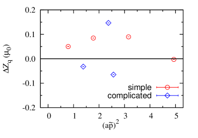
(a) c-mom

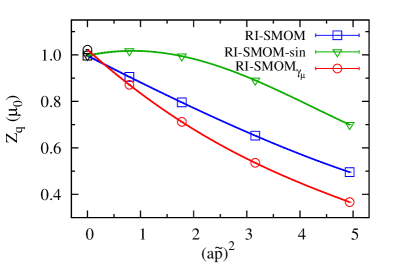
(b) s-mom

Figure 2: P-fit results for $Z_{q}$ in the RI-SMOM schemes: 2(a) results of $\Delta Z_{q}$ with both simple and complicated momenta, and 2(b) $Z_{q}$ fits with only simple momenta. Here, c-mom (s-mom) represents complicated (simple) momenta.

2.5 Results: Momentum Fit for $Z_{m}$

Results for $Z_{m}$ are obtained by dividing $\Gamma^{S\otimes S}_{B}$ by $\Gamma^{V\otimes S}_{B}$. Hence, most of lattice artifacts are canceled between the numerator and denominator, which allows us to fit the data of both simple and complicated momenta to the fitting functional form:

$$f_{(2)} =c_{1}+c_{2}(a\widetilde{p})^{2}+c_{3}(a\widetilde{p})^{4}/(a\widetilde{p})^{2}$$ (7)

$$f_{(4)} =f_{(2)}+c_{4}((a\widetilde{p})^{2})^{2}+c_{5}((a\widetilde{p})^{4})+c_{6}((a\widetilde{p})^{4}/(a\widetilde{p})^{2})^{2}+c_{7}(a\widetilde{p})^{6}/(a\widetilde{p})^{2}$$ (8)

$$f_{(6)} =f_{(4)}+c_{8}((a\widetilde{p})^{2})^{3}+c_{9}(a\widetilde{p})^{2}(a\widetilde{p})^{4}+c_{10}((a\widetilde{p})^{4})^{2}/(a\widetilde{p})^{2}+c_{11}(a\widetilde{p})^{6}$$

$$\hskip 28.45274pt+c_{12}(a\widetilde{p})^{4}(a\widetilde{p})^{6}/((a\widetilde{p})^{2})^{2}+c_{13}(a\widetilde{p})^{8}/(a\widetilde{p})^{2}$$ (9)

where the sub-index $n$ of $f_{(n)}$ represents the order $\mathcal{O}((a\widetilde{p})^{n})$ of highest order terms included in the fit.

In Fig. 3, we present fitting results for $Z_{m}$ in the RI-SMOM${}_{\gamma_{\mu}}$ scheme. In this fit, we choose $f_{(4)}$ as the fitting function and impose the Bayesian constraints on $c_{4-7}$: $c_{i}=0\pm\sigma$ and $\sigma=1/(a\Lambda)^{4}$ with $\Lambda=4$ GeV for $i=4,\ldots,7$. On the MILC coarse lattice, this means that $c_{i}=0\pm 0.03$. We define $x_{m}$ as

$$x_{m} =Z_{m}(\text{data})-\langle c_{3}\rangle(a\widetilde{p})^{4}/(a\widetilde{p})^{2}-\langle c_{5}\rangle(a\widetilde{p})^{4}-\langle c_{6}\rangle((a\widetilde{p})^{4}/(a\widetilde{p})^{2})^{2}-\langle c_{7}\rangle(a\widetilde{p})^{6}/(a\widetilde{p})^{2}\;.$$ (10)

Hence, $x_{m}$ represents $Z_{m}$ with its lattice artifacts removed and $\Delta Z_{m}=Z_{m}(\text{data})-f_{(4)}$ corresponds to the fitting quality. We present $x_{m}$ on Fig. 3 3(a), and $\Delta Z_{m}$ on Fig. 3 3(b). In this fit, $\chi^{2}/\text{d.o.f.}=0.20(28)$.

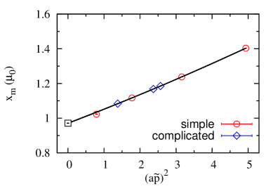
(a) $x_{m}$

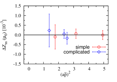
(b) $\Delta Z_{m}$

Figure 3: P-fit results for $Z_{m}$ in the RI-SMOM${}_{\gamma_{\mu}}$ scheme: 3(a) $x_{m}$ and 3(b) $\Delta Z_{m}$.

In Fig. 4, we show results for $Z_{m}$ in the RI-SMOM scheme. In this fit, we choose $f_{(6)}$ as the fitting function and impose the Bayesian prior conditions on $c_{4-13}$. For $c_{4-6}$, $c_{i}=0\pm\sigma_{4}$ and $\sigma_{4}=1/(a\Lambda)^{4}$ with $\Lambda=4$ GeV. For $c_{7}$, $c_{7}=0\pm 3\sigma_{4}$, in order to make the fitting results consistent with the constraints. For $c_{8-13}$, $c_{j}=0\pm\sigma_{6}$ and $\sigma_{6}=1/(a\Lambda)^{6}$ with $\Lambda=4$ GeV. On the MILC coarse lattice, this means that $\sigma_{4}=0.03$ and $\sigma_{6}=0.005$. We define $y_{m}$ as

$$y_{m} =Z_{m}(\text{data})-\langle c_{3}\rangle(a\widetilde{p})^{4}/(a\widetilde{p})^{2}-\langle c_{5}\rangle(a\widetilde{p})^{4}-\langle c_{6}\rangle((a\widetilde{p})^{4}/(a\widetilde{p})^{2})^{2}-\langle c_{7}\rangle(a\widetilde{p})^{6}/(a\widetilde{p})^{2}$$

$$\hskip 14.22636pt-\langle c_{9}\rangle(a\widetilde{p})^{2}(a\widetilde{p})^{4}-\langle c_{10}\rangle((a\widetilde{p})^{4})^{2}/(a\widetilde{p})^{2}-\langle c_{11}\rangle(a\widetilde{p})^{6}$$

$$\hskip 14.22636pt-\langle c_{12}\rangle(a\widetilde{p})^{4}(a\widetilde{p})^{6}/((a\widetilde{p})^{2})^{2}-\langle c_{13}\rangle(a\widetilde{p})^{8}/(a\widetilde{p})^{2}\;.$$ (11)

Thus, $y_{m}$ represents $Z_{m}$ with its lattice artifacts removed. We also redefine $\Delta Z_{m}=Z_{m}(\text{data})-f_{(6)}$. We show $y_{m}$ on Fig. 4 4(a) and $\Delta Z_{m}$ on Fig. 4 4(b). The fitting quality is $\chi^{2}/\text{d.o.f.}=1.15(86)$.

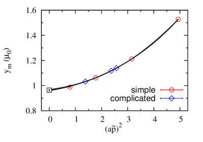
(a) $y_{m}$

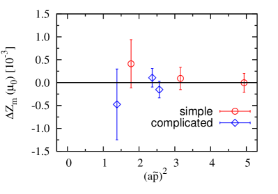
(b) $\Delta Z_{m}$

Figure 4: P-fit results for $Z_{m}$ in the RI-SMOM scheme: 4(a) $y_{m}$ and 4(b) $\Delta Z_{m}$.

In Table 3, we summarize our preliminary results for $Z_{q}$ and $Z_{m}$ at $\mu=3$ GeV in the ${\overline{\text{MS}}}$ scheme.

int. scheme	$Z_{q}^{{\overline{\text{MS}}}}(\mu)$	$Z_{m}^{{\overline{\text{MS}}}}(\mu)$
$\textrm{RI-SMOM}_{\gamma_{\mu}}$	1.053(1)(15)	0.920(1)(14)
RI-SMOM	0.984(1)(4)	0.948(7)(14)
RI-SMOM-sin	0.984(2)(4)	0.976(7)(15)
RI-MOM	1.060(8)(4)	0.94(11)(0)

Table 3: Results of $Z_{q}$ and $Z_{m}$ in the ${\overline{\text{MS}}}$ scheme at $\mu=3$ GeV. They are obtained using the RI-SMOM schemes as an intermediate scheme. The first error is purely statistical, and the second systematic which comes from the truncation of higher order terms in perturbative matching. Here, all the results are preliminary in that the error budget is incomplete.

3 Gribov Uncertainty in RI-MOM

Landau gauge fixing is done by maximizing the functional $F$: $F=1/(2N_{c}\cdot 4V)\sum_{\mu,x}\textrm{Tr}[U_{\mu}(x)+U_{\mu}(x)^{\dagger}]$. where $N_{c}=3$, and $V$ is 4-dimensional volume, and $U_{\mu}$ is a gluon link field. In practice, the gauge fixing condition is checked by monitoring $\theta\equiv 1/(N_{c}V)\cdot\sum_{x}\textrm{Tr}[\Delta(x)\Delta^{\dagger}(x)]$ such that $\theta<10^{-14}$. Here, note that $\Delta(x)\equiv 16iN_{c}V\frac{\delta F}{\delta\omega^{a}(x)}T^{a}$. We use the Fourier accelerated steepest descent algorithm [9] to maximize $F$.

It is well known that Landau gauge fixing has Gribov ambiguity [6]: two independent gauge configurations (Gribov copies) can satisfy the same gauge fixing condition. In general, we can distinguish different Gribov copies from one another by monitoring their values of $F$ since $F$ is gauge-dependent. We start with a mother gauge configuration which has $F=F_{m}$. Then we apply randomly gauge transformation to the mother in order to produce a daughter configuration which has $F=F_{d}\neq F_{m}$. We repeat this procedure 100 times to generate 100 daughter configurations. Then, we pick the daughter with $F_{d}^{\text{max}}$ which maximize $\delta F=|F_{m}-F_{d}|$. We measure $Z_{q}$ on the mother and the daughter with $F=F_{d}^{\text{max}}$.

In Fig. 5, we present results for $\Delta Z_{q}^{\text{G}}=Z_{q}(\text{daughter})-Z_{q}(\text{mother})$. It turns out that the systematic error due to Gribov ambiguity is negligibly small ($\approx 0.02\%$).

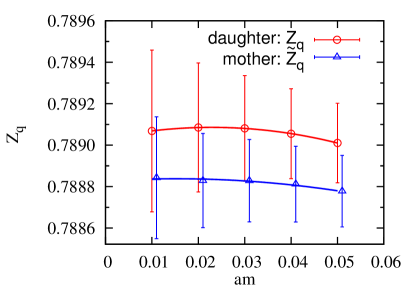
(a) m-fit

(b) p-fit

Figure 5: Gribov ambiguity in $Z_{q}$: 5(a) m-fit and 5(b) p-fit of $\Delta Z_{q}^{G}=\widetilde{Z}_{q}-Z_{q}$.

References

[1]
J. A. Bailey, Y.-C. Jang, W. Lee, and S. Park Phys. Rev.D92 (2015)
034510, [1503.05388].
[2]
T. Bae et al.Phys. Rev.D89 (2014), no. 7 074504,
[1402.0048].