FTPI–MINN–15/47

UMN–TH–3510/15

KIAS-P15063

The ATLAS Diboson Resonance in
Non-Supersymmetric SO(10)

Jason L. Evans^1,2, Natsumi Nagata², Keith A. Olive², and Jiaming Zheng²

¹School of Physics, KIAS, Seoul 130-722, Korea
²William I. Fine Theoretical Physics Institute, School of Physics and Astronomy, University of Minnesota, Minneapolis, Minnesota 55455, USA

SO(10) grand unification accommodates intermediate gauge symmetries with which gauge coupling unification can be realized without supersymmetry. In this paper, we discuss the possibility that a new massive gauge boson associated with an intermediate gauge symmetry explains the excess observed in the diboson resonance search recently reported by the ATLAS experiment. The model we find has two intermediate symmetries, $\text{SU}(4)_{C}\otimes\text{SU}(2)_{L}\otimes\text{SU}(2)_{R}$ and $\text{SU}(3)_{C}\otimes\text{SU}(2)_{L}\otimes\text{SU}(2)_{R}\otimes\text{U}(1)_{B-L}$, where the latter gauge group is broken at the TeV scale. This model achieves gauge coupling unification with a unification scale sufficiently high to avoid proton decay. In addition, this model provides a good dark matter candidates, whose stability is guaranteed by a $\mathbb{Z}_{2}$ symmetry present after the spontaneous breaking of the intermediate gauge symmetries. We also discuss prospects for testing these models in the forthcoming LHC experiments and dark matter detection experiments.

1 Introduction

Grand unification [1] is considered to be one of the most promising frameworks for physics beyond the Standard Model (SM). SO(10) Grand Unified Theories (GUTs) [2, 3, 4] have many especially attractive features. First, the full set of SM fermions of each generation together with a right-handed neutrino is embedded into a single ${\bf 16}$ chiral representation of SO(10). Second, anomaly cancellation in the SM can be understood naturally since SO(10) is free from anomalies. Third, gauge coupling unification can be realized without relying on supersymmetry, if there are intermediate-scale gauge symmetries [5]. Majorana mass terms of right-handed neutrinos can be generated at an intermediate scale, which may explain the smallness of neutrino masses. These interesting aspects have stimulated many extensive studies of SO(10) GUTs [6, 7, 8, 9].

In addition, SO(10) GUTs with intermediate gauge symmetries predict new gauge bosons whose masses are of the order of the breaking scales of the corresponding gauge symmetries. The breaking scale of these intermediate gauge symmetries affects the running of the gauge couplings. These scales can be determined by requiring gauge coupling unification, which is highly dependent on the symmetry-breaking pattern and matter content of the model. However, we will show that it is possible to obtain a model containing TeV-scale gauge bosons accessible at the LHC, for a particular choice of the intermediate gauge symmetries and particle content.

In this paper, we consider non-supersymmetric SO(10) GUT models with an intermediate gauge symmetry showing up around the TeV scale, and discuss the possibility that a new gauge boson associated with the intermediate gauge symmetry can explain the anomalous diboson events recently reported by the ATLAS collaboration [10]. We will discuss a model with two intermediate symmetries, $\text{SU}(4)_{C}\otimes\text{SU}(2)_{L}\otimes\text{SU}(2)_{R}$ which is then broken to $\text{SU}(3)_{C}\otimes\text{SU}(2)_{L}\otimes\text{SU}(2)_{R}\otimes\text{U}(1)_{B-L}$. The unified and intermediate scales are determined by the renormalization group (RG) running of the gauge couplings and depend on the matter content of the theory. In the model discussed, the GUT scale is of order $10^{17}$ GeV and is high enough so that the proton decay bounds can be evaded. The first intermediate scale is of order $10^{9}$ GeV and is high enough that constraints from leptoquarks are satisfied. The second intermediate scale lies around a few TeV and the charged gauge bosons of $\text{SU}(2)_{R}$, $W_{R}^{\pm}$, can have a mass $\sim 2$ TeV and may explain the excess observed in the ATLAS diboson resonance search [10]. The possibility of this new charged gauge boson explaining the diboson anomaly is discussed in Refs. [11, 12, 13, 14, 15, 16]. We will see that $W_{R}^{\pm}$ in this model can also reproduce the diboson excess. Furthermore, this $W_{R}^{\pm}$ may explain another anomaly observed by the CMS collaboration in the right-handed neutrino searches with a dijet and a dilepton final state [17], as we will discuss below. Our model also predicts an additional massive boson: a neutral gauge boson $Z_{R}$. Detection of this $Z_{R}$ would be a smoking-gun signature of our model. The masses of the $Z_{R}$ can be heavier than the $W_{R}^{\pm}$ mass, and thus evades the current LHC bound. However, it may be in reach of Run-II of the LHC, as we will discuss.

Our model also contains a promising dark matter candidate. The dark matter candidate is stabilized by a residual $\mathbb{Z}_{2}$ symmetry arising after the SO(10) symmetry has been completely broken to the SM gauge symmetries [18, 19, 20, 21, 22, 23, 24, 25, 26, 27]. This residual $\mathbb{Z}_{2}$, as it turns out, is equivalent to matter parity [28]. It is tantalizing that the presence of this dark matter candidate is essential for the model to achieve gauge coupling unification. An integral part of obtaining gauge coupling unification in this set up is an intermediate scale of order a TeV, a second intermediate scale large enough to suppress the effects of leptoquarks, and a GUT scale which is large enough to avoid proton decay. Given these conditions, the required matter content at low energies is severely restricted, and thus it is highly non-trivial that our model contains a good dark matter candidate. The presence of dark matter gives us another opportunity to test this model; we can probe the dark matter candidate predicted in this model in dark matter detection experiments. We also discuss this prospect in what follows. Combining dark matter search results with those obtained at the LHC experiments, we may be able to test our model in near future.

This paper is organized as follows. We first describe our model in the next section. Then, in Sec. 3, we briefly review the ATLAS diboson anomaly, and show that the $W^{\pm}_{R}$ in our model can explain the diboson anomaly. We also discuss the present constraints on our models from various experiments and consider the testability of this model in future LHC experiments and dark matter searches. Finally, we conclude in Sec. 4.

2 The Model

In this section, we describe the specific SO(10) model used in this analysis. This model is obtained in a similar manner to that discussed in Ref. [25], except now we allow for two intermediate scales. To obtain these intermediate scales, we need to arrange some Higgs fields to acquire vacuum expectation values (VEVs) in specific directions at particular scales. Throughout this work, we make an assumption on the Higgs field content. We assume that at each intermediate scale the Higgs fields present are components of the SO(10) multiplets that have VEVs equal to or less then the corresponding intermediate scale. The other components have masses of order of the previous symmetry-breaking scale. We also allow for a light SO(10) component which could be dark matter.

Before we get into the details of our model, we first discuss the necessity for two intermediate scales. If there were only one intermediate scale and we wished to explain the ATLAS diboson excess, we would have to choose the TeV scale. For intermediate gauge symmetries which include the SU(4)_C subgroup, this choice turns out to be problematic since the breaking of the SU(4)_C subgroup generates a vector leptoquark at that intermediate scale. Since this leptoquark interacts with both left- and right-handed fermions, it will generate excessively large contributions to the meson decays (see, e.g., Ref. [32]). In fact, one can show that no tuning can simultaneously tune away the contribution of a vector leptoquark to the Kaon decays $K^{+}\to\pi^{+}\bar{e}\mu$ and $K_{L}\to\bar{e}\mu$ by exploiting the contributions of the scalar leptoquarks contained inside the Higgs fields. If the intermediate gauge symmetries do not contain the SU(4)_C subgroup, on the other hand, we find that we cannot obtain gauge coupling unification with a sufficiently high GUT scale since there are no new contributions to the running of the SU(3)_C gauge coupling constant. This makes it impossible to get the intermediate scale to be around the TeV scale while maintaining gauge coupling unification with a sufficiently high GUT scale. These problems, however, can be evaded if a two step breaking pattern is considered. The vector leptoquark then has a mass of order of the larger intermediate scale. This larger intermediate scale generates a mass for the vector leptoquarks which is high enough to avoid constraints coming from meson decays but low enough that the vector leptoquarks still contribute significantly to the running of the SU(3)_C gauge coupling.

The breaking pattern of our model, with two intermediate gauge symmetries, is from SO(10) to $\text{SU}(4)_{C}\otimes\text{SU}(2)_{L}\otimes\text{SU}(2)_{R}$ which is then broken to $\text{SU}(3)_{C}\otimes\text{SU}(2)_{L}\otimes\text{SU}(2)_{R}\otimes\text{U}(1)_{B-L}$. For the breaking pattern we consider, SO(10) is broken by the VEV of the $({\bf 1},{\bf 1},{\bf 1})$ component of a 210 into $\text{SU}(4)_{C}\otimes\text{SU}(2)_{L}\otimes\text{SU}(2)_{R}$. This symmetry is then subsequently broken by a VEV of the $({\bf 15},{\bf 1},{\bf 1})$ component of the same 210 to $\text{SU}(3)_{C}\otimes\text{SU}(2)_{L}\otimes\text{SU}(2)_{R}\otimes\text{U}(1)_{B-L}$. Importantly, the $({\bf 1},{\bf 1},{\bf 1})$ component of the 210 breaks $D$-parity [33] at the GUT scale, and thus the low-energy effective theory does not exhibit a left-right symmetry [34]. Finally, this gauge group is broken to the SM gauge symmetries at the TeV scale by the $({\bf 1},{\bf 1},{\bf 3},+2)$ component of a ${\bf 126}$. However, there remains a $\mathbb{Z}_{2}$ symmetry coming from U(1)_B-L since the $B-L$ charge of this component of the ${\bf 126}$ is $2$ [18, 19, 20, 21]. The $({\bf 1},{\bf 1},{\bf 3},0)$ component of the ${\bf 210}$ also breaks $\text{SU}(3)_{C}\otimes\text{SU}(2)_{L}\otimes\text{SU}(2)_{R}\otimes\text{U}(1)_{B-L}$, but does not break the $\mathbb{Z}_{2}$ symmetry since its $B-L$ charge is zero. In summary, we consider the following symmetry-breaking chain:

$$\text{SO}(10) \stackrel{{\scriptstyle\langle{\bf 210}\rangle}}{{\longrightarrow}}\text{SU}(4)_{C}\otimes\text{SU}(2)_{L}\otimes\text{SU}(2)_{R}$$

$$\stackrel{{\scriptstyle\langle{\bf 210}\rangle}}{{\longrightarrow}}\text{SU}(3)_{C}\otimes\text{SU}(2)_{L}\otimes\text{SU}(2)_{R}\otimes\text{U}(1)_{B-L}$$

$$\xrightarrow{\langle{\bf 126}\rangle~{}\langle{\bf 210}\rangle}~{}\text{SU}(3)_{C}\otimes\text{SU}(2)_{L}\otimes\text{U}(1)_{Y}\otimes\mathbb{Z}_{2}~{}.$$ (1)

Under the remnant $\mathbb{Z}_{2}$ symmetry, which is found to be equivalent to matter parity $P_{M}=(-1)^{3(B-L)}$ [28], the SM fermions are odd while the SM Higgs is even. Therefore, a scalar boson (fermion) can be stable if it is odd (even) under this $\mathbb{Z}_{2}$ symmetry. If such a particle is electrically and color neutral, it can be a good dark matter candidate [22, 23]. For a detailed discussions on this class of dark matter candidates in SO(10) GUTs, see Refs. [24, 25].

The low-energy matter content of this model, beyond the SM fermions and right-handed neutrinos (which are embedded into three 16 representations), is given in Table 1. Here, the first, second, and third columns show the SO(10), $\text{SU}(4)_{C}\otimes\text{SU}(2)_{L}\otimes\text{SU}(2)_{R}$, and $\text{SU}(3)_{C}\otimes\text{SU}(2)_{L}\otimes\text{SU}(2)_{R}\otimes\text{U}(1)_{B-L}$ quantum numbers of the particles, respectively, while the fourth column represents their $\mathbb{Z}_{2}$ charges. The subscripts $C$ and $D$ refer to complex and Dirac respectively. Most of the components of the 210 have GUT scale masses and do not affect our analysis. In this model, the (15, 1, 1)_C component of 210_C has a mass similar to the $\text{SU}(4)_{C}\otimes\text{SU}(2)_{L}\otimes\text{SU}(2)_{R}$ breaking scale, as its VEV breaks the symmetry. Similarly, the components of(15, 1, 3) $\in$ 210 and ($\overline{\bf 10}$, 1, 3) $\in$ 126 charged under color have masses of order the higher intermediate scale breaking. The components in the third column of the table are those components which are fine-tuned to have masses lighter than this scale. Among the light fields are the (1, 1, 3, $+2$)_C and the (1, 1, 3, 0)_C which obtain VEVs and break the $\text{SU}(3)_{C}\otimes\text{SU}(2)_{L}\otimes\text{SU}(2)_{R}\otimes\text{U}(1)_{B-L}$ symmetry to the SM symmetries. The components of these fields which are not eaten by the gauge bosons receive masses of order of the VEV breaking this symmetry. The rest of the Higgs fields listed in the table are responsible for breaking the electroweak symmetry and have masses of order the electroweak scale. Also listed in the table is an $\text{SU}(2)_{L}$ triplet Dirac fermion which can be a viable dark matter candidate and could originate from a 45 of SO(10). The remaining components of the 45 (beyond the triplet) should all have GUT scale masses. In summary, the states in column 2 affect the running of the gauge couplings between the high intermediate scale and the GUT scale, and those in column 3 affect the running between the TeV scale and the high intermediate scale. The particles in the third column and green shaded rows contribute to the running of the gauge couplings below the TeV scale. This leads to a theory below the TeV scale with the SM fermions and four doublet Higgs bosons. A similar decomposition can be made for the the gauge bosons; the $({\bf 6},{\bf 2},{\bf 2})$ component of the SO(10) gauge boson, ${\bf 45}$, is around the GUT scale, while the other components, the SU(4)_C, SU(2)_L, and SU(2)_R gauge bosons, are massless at this stage of the GUT symmetry breaking. A part of the SU(4)_C gauge bosons, the vector leptoquark, obtains a mass of the order of the higher intermediate scale, as we will see below.

Table 1: Particle content of our model. The first, second, and third columns show the SO(10), $\text{SU}(4)_{C}\otimes\text{SU}(2)_{L}\otimes\text{SU}(2)_{R}$, and $\text{SU}(3)_{C}\otimes\text{SU}(2)_{L}\otimes\text{SU}(2)_{R}\otimes\text{U}(1)_{B-L}$ quantum numbers of the particles, respectively, while the forth column represents their $\mathbb{Z}_{2}$ charges. The orange (green) shaded fields acquire VEVs of about a few TeV (the electroweak scale), and the blue shaded particle contains a dark matter candidate. The $({\bf 15},{\bf 1},{\bf 1})_{C}$ of the 210_C lies around the $\text{SU}(4)_{C}\otimes\text{SU}(2)_{L}\otimes\text{SU}(2)_{R}$ breaking scale, and none of its components appears below this scale.

SO(10)	$\text{SU}(4)_{C}\otimes\text{SU}(2)_{L}\otimes\text{SU}(2)_{R}$	$\text{SU}(3)_{C}\otimes\text{SU}(2)_{L}\otimes\text{SU}(2)_{R}\otimes\text{U}(1)_{B-L}$	$\mathbb{Z}_{2}$
210C	(15, 1, 1)C	–	$+$
126C	($\overline{\bf 10}$, 1, 3)C	(1, 1, 3, $+2$)C	$+$
210C	(15, 1, 3)C	(1, 1, 3, 0)C	$+$
10C	(1, 2, 2)C	(1, 2, 2, 0)C	$+$
126C	(15, 2, 2)C	(1, 2, 2, 0)C	$+$
45D	(1, 3, 1)D	(1, 3, 1, 0)D	$+$

The mass of the dark matter candidate is fixed by requiring that its thermal relic abundance agree with the observed dark matter density $\Omega_{\text{DM}}h^{2}\simeq 0.12$ [35]. The thermal relic abundance of any DM candidate is determined by its thermally averaged annihilation cross section $\sigma_{\text{ann}}$ times the relative velocity between the initial particles, $v_{\text{rel}}$, via the following relation:

$$\Omega_{\text{DM}}h^{2}\simeq\frac{3\times 10^{-27}~{}\text{cm}^{3}~{}\text{s}^{-1}}{\langle\sigma_{\text{ann}}v_{\text{rel}}\rangle}~{}.$$ (2)

Here, the brackets signify a thermal average. In the case of an SU(2)_L triplet Dirac fermion dark matter candidate with zero hypercharge, the $s$-wave annihilation cross section is given by [36]

$$\langle\sigma_{\text{ann}}v_{\text{rel}}\rangle\simeq\frac{37g_{2}^{4}}{192\pi m^{2}_{\text{DM}}}~{},$$ (3)

where $g_{2}$ denotes the SU(2)_L gauge coupling constant and $m_{\text{DM}}$ is the dark matter mass. From Eqs. (2) and (3), we obtain $m_{\text{DM}}\simeq 2$ TeV. However, it is known that the non-perturbative Sommerfeld effect significantly enhances the annihilation cross section [37], which results in a smaller cross section, and thus larger dark matter mass, needed to reproduce the correct dark matter density. As far as we know, the thermal relic abundance of a triplet Dirac fermion has not been computed yet with the Sommerfeld enhancement effect included. However, we expect that the favored mass for a Dirac triplet is smaller than that for a Majorana triplet (which was found to be $\sim 2.7$ TeV [38]), since the thermally-averaged annihilation cross section of Dirac dark matter is a factor of two smaller than that of Majorana dark matter.

In Fig. 1, we show a plot of the running of the gauge coupling constants in this model. Here, we set the masses of the fields in the third column in Table 1 to be 1.9 TeV. In this figure, we show the running of the inverse of $\alpha_{a}\equiv g_{a}^{2}/(4\pi)$ $(a=1,2,3)$ with $g_{1}$, $g_{2}$, and $g_{3}$ corresponding to the U(1)_Y, SU(2)_L, and SU(3)_C gauge coupling constants, respectively. The definitions of these gauge couplings in the $\text{SU}(4)_{C}\otimes\text{SU}(2)_{L}\otimes\text{SU}(2)_{R}$ theory are given by

$$\frac{1}{\alpha_{1}}\equiv\frac{3}{5}\frac{1}{\alpha_{2R}}+\frac{2}{5}\frac{1}{\alpha_{4}}~{},~{}~{}~{}~{}\alpha_{2}\equiv\alpha_{2L},~{}~{}~{}~{}\alpha_{3}\equiv\alpha_{4}~{},$$ (4)

where $\alpha_{4}$, $\alpha_{2L}$, and $\alpha_{2R}$ represent the SU(4)_C, SU(2)_L, and SU(2)_R gauge couplings, respectively, while those in the $\text{SU}(3)_{C}\otimes\text{SU}(2)_{L}\otimes\text{SU}(2)_{R}\otimes\text{U}(1)_{B-L}$ theory are

$$\frac{1}{\alpha_{1}}\equiv\frac{3}{5}\frac{1}{\alpha_{2R}}+\frac{2}{5}\frac{1}{\alpha_{B-L}}~{},~{}~{}~{}~{}\alpha_{2}\equiv\alpha_{2L},$$ (5)

where $\alpha_{B-L}$ is the U(1)_B-L gauge coupling. Using the weak scale values of the gauge couplings as inputs and insisting on unification of the coupling constants at some high energy scale, allows us to use the three RGEs to solve for the higher intermediate scale, the GUT scale, and the value of the the unified gauge coupling at the GUT scale (recall that we have fixed the value of the lower intermediate scale). From this figure, we find that the GUT scale in this model is $9.8\times 10^{16}$ GeV, which is high enough to avoid proton decay constraints. The $\text{SU}(4)_{C}\otimes\text{SU}(2)_{L}\otimes\text{SU}(2)_{R}$ breaking scale is determined to be $\simeq 7.2\times 10^{8}$ GeV. The $\text{SU}(3)_{C}\otimes\text{SU}(2)_{L}\otimes\text{SU}(2)_{R}\otimes\text{U}(1)_{B-L}$ gauge coupling constants at 1.9 TeV are found to be

$$g_{B-L}\simeq 0.58~{},~{}~{}~{}~{}g_{2L}\simeq 0.64~{},~{}~{}~{}~{}g_{2R}\simeq 0.42~{},~{}~{}~{}~{}g_{3}\simeq 1.03~{}.$$ (6)

The value of $g_{2R}$ above will be important when we discuss the diboson anomaly.

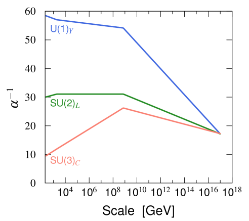
Figure 1: Running of gauge couplings in our model. Here, we set the masses of the fields in the third column in Table 1 to be 1.9 TeV.

In this model, only $W_{R}^{\pm}$ and $Z_{R}$ lie around the TeV scale, while the vector leptoquarks have masses of ${\cal O}(10^{\text{8--9}})$ GeV. The scalar leptoquarks arising from the $({\bf 15},{\bf 1},{\bf 1})_{C}$ and $({\bf 15},{\bf 1},{\bf 3})_{C}$ of the ${\bf 210}_{C}$ and $(\overline{\bf 10},{\bf 1},{\bf 3})_{C}$ and $({\bf 15},{\bf 2},{\bf 2})_{C}$ of the ${\bf 126}_{C}$ also have a mass of order this scale. The masses of $W_{R}^{\pm}$ and $Z_{R}$ are computed to be

$$m_{W_{R}}^{2} \simeq g_{2R}^{2}\left[(v_{R}^{\bf 10})^{2}+(v_{R}^{\bf 15})^{2}\right]~{},$$

$$m_{Z_{R}}^{2} \simeq 2\left(g_{2R}^{2}+\frac{3}{2}g_{B-L}^{2}\right)(v_{R}^{\bf 10})^{2}~{},$$ (7)

where

$$\langle({\bf 1},{\bf 1},{\bf 3},+2)_{C}\rangle=T_{-}v_{R}^{\bf 10}~{},~{}~{}~{}~{}~{}~{}\langle({\bf 1},{\bf 1},{\bf 3},0)_{C}\rangle=T_{3}v_{R}^{\bf 15}~{}.$$ (8)

Here, $T_{a}=\tau_{a}/2$ ($a=1,2,3$) with $\tau_{a}$ the Pauli matrices and $T_{-}\equiv T_{1}-iT_{2}$, and we have neglected the contribution of the electroweak-scale VEVs for simplicity. On the other hand, the vector leptoquarks, whose quantum numbers under the $\text{SU}(3)_{C}\otimes\text{SU}(2)_{L}\otimes\text{U}(1)_{Y}$ symmetry are $({\bf 3},{\bf 1},+2/3)\oplus(\overline{\bf 3},{\bf 1},-2/3)$, acquire a mass of

$$m_{V_{\text{LQ}}}^{2}\simeq\frac{2}{3}g_{4}^{2}\left(v_{422}^{\bf 15}\right)^{2}~{},$$ (9)

with

$$\langle({\bf 15},{\bf 1},{\bf 1})_{C}\rangle=X_{B-L}v_{422}^{\bf 15}~{},$$ (10)

where $X_{B-L}$ is the SU(4)_C generator corresponding to the $B-L$ charge, i.e. $\sqrt{\frac{3}{8}}(B-L)$. As the $({\bf 15},{\bf 1},{\bf 1})_{C}$ VEV $v_{422}^{\bf 15}$ sets the $\text{SU}(4)_{C}\otimes\text{SU}(2)_{L}\otimes\text{SU}(2)_{L}$ breaking scale, $m_{V_{\text{LQ}}}$ is as high as $\sim 10^{9}$ GeV. The masses of the scalar leptoquarks are dependent on the couplings in the scalar potential; generically, they are also ${\cal O}(v^{\bf 15}_{422})$.

Since the gauge couplings $g_{B-L}$ and $g_{2R}$ are determined, and given in Eq. (6), if we fix the $W_{R}^{\pm}$ mass, then we obtain the $Z_{R}$ mass as a function of $v_{R}^{\bf 15}$. We show this in Fig. 2 setting $m_{W_{R}}=1.9$ TeV. It is found that the $Z_{R}$ mass is relatively small; in particular, $m_{Z_{R}}$ can be much smaller than that predicted in the minimal left-right symmetric model with a single SU(2)_R triplet Higgs field [34], which is reproduced if one takes $v_{R}^{\bf 15}=0$. This distinguishing feature can be tested at the LHC. Currently, the most stringent bound on $m_{Z_{R}}$ is given by the resonance searches in Drell-Yan processes [39, 40]. The CMS collaboration gives the most severe limits on this process [40]. Using this analysis, it is found that the present lower bound on the $Z_{R}$ mass in our model is $m_{Z_{R}}\gtrsim 3.05$ TeV. We show this limit by the blue shaded area in Fig. 2. We find that $m_{Z_{R}}$ in our model can satisfy this constraint over a wide range of $v_{R}^{\bf 15}$. The rest of allowed mass range, $3.05$ TeV $\lesssim m_{Z_{R}}\lesssim 5.2$ TeV, can be reached at Run-II of the LHC. For example, the 14 TeV LHC run with an integrated luminosity of 300 fb^-1 can probe the entire parameter space in Fig. 2 [42]. Finally, we note in passing that the $Z_{R}$ in our model may explain the dielectron event at 2.9 TeV recently announced by the CMS collaboration [43], although there are inconsistencies with the CMS dilepton bound. These $Z_{R}$ signatures can possibly be tested in the near future.

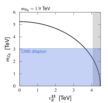
Figure 2: $m_{Z_{R}}$ as a function of $v_{R}^{\bf 15}$. Here, we set $m_{W_{R}}=1.9$ TeV. The gray shaded region predicts right-handed neutrino masses to be lighter than the $W_{R}^{\pm}$ mass when $y_{\Delta}<1$, while the blue shaded area is excluded by the CMS dilepton searches [40].

The VEVs of the bi-doublet Higgs fields $\Phi_{\bf 1}$ and $\Phi_{\bf 15}$ originally coming from $({\bf 1},{\bf 2},{\bf 2})_{C}$ and $({\bf 15},{\bf 2},{\bf 2})_{C}$ of the ${\bf 10}_{C}$ and ${\bf 126}_{C}$, respectively, induce mixing between the SU(2)_L and SU(2)_R gauge bosons. Through this mixing, $W_{R}^{\pm}$ can decay into a $W$ and $Z$. Therefore, by appropriately choosing the mixing angle, we may explain the diboson excess observed in the ATLAS experiment [10], as we discuss in the next section.

In addition, the VEVs of $\Phi_{\bf 1}$, $\Phi_{\bf 15}$, and $\Delta=({\bf 1},{\bf 1},{\bf 3},+2)_{C}$ from the ${\bf 126}_{C}$ generate the fermion mass terms via Yukawa interactions. At the TeV scale, the relevant Yukawa terms are given by

$${\cal L}_{\text{Yukawa}}= -\overline{Q_{L}}\left(y^{Q}_{\bf 1}\Phi_{\bf 1}+\widetilde{y}^{Q}_{\bf 1}\widetilde{\Phi}_{\bf 1}\right)Q_{R}-\frac{1}{\sqrt{24}}~{}\overline{Q_{L}}\left(y_{\bf 15}^{Q}\Phi_{\bf 15}+\widetilde{y}^{Q}_{\bf 15}\widetilde{\Phi}_{\bf 15}\right)Q_{R}$$

$$-\overline{L_{L}}\left(y^{L}_{\bf 1}\Phi_{\bf 1}+\widetilde{y}^{L}_{\bf 1}\widetilde{\Phi}_{\bf 1}\right)L_{R}+\sqrt{\frac{3}{8}}~{}\overline{L_{L}}\left(y_{\bf 15}^{L}\Phi_{\bf 15}+\widetilde{y}^{L}_{\bf 15}\widetilde{\Phi}_{\bf 15}\right)L_{R}$$

$$-y_{\Delta}\overline{L_{R}^{c}}\Delta L_{R}+\text{h.c.}~{},$$ (14)

where $c$ denotes the charge conjugation and $\widetilde{\Phi}_{\bf 1,15}\equiv\tau_{2}\Phi^{*}_{\bf 1,15}\tau_{2}$. Here, we note that $y_{\bf 1,15}^{Q}=y_{\bf 1,15}^{L}$ and $\widetilde{y}_{\bf 1,15}^{Q}=\widetilde{y}_{\bf 1,15}^{L}$ hold at the first intermediate scale because of the SU(4)_C symmetry. After the bi-doublet fields acquire VEVs, $\langle\Phi_{{\bf 1,15}}\rangle=\text{diag}(v_{u}^{{\bf 1,15}},v_{d}^{{\bf 1,15}})$, the operators including these VEVs generate a Dirac mass term for the charged SM fields, while the VEV of $\Delta$ gives rise to a Majorana mass terms for the right-handed neutrinos. Since both the $\Phi_{\bf 1,15}$ and $\Phi_{\bf 1,15}^{*}$ can couple to the SM fermions, with different Yukawa couplings, the form of the Yukawa couplings is similar to that of a generic two-Higgs doublet model. This Yukawa structure in general suffers from large flavor-changing neutral currents [44, 45, 46]. In this work, we just assume that the Yukawa couplings are appropriately aligned so that the flavor-changing processes induced by the exchange of the Higgs fields are sufficiently suppressed.

As mentioned above, the lepton Yukawa couplings are equal to the quark Yukawa couplings at the first intermediate scale. As a result, the Dirac Yukawa couplings for neutrinos are sizable. This is potentially problematic since the Majorana masses for right-handed neutrinos in our model are at the TeV scale. To discuss this point, let us investigate the neutrino mass terms. The masses of light neutrinos in our model are given by the ordinary seesaw relation [49],

$$m_{\nu}\simeq-m_{D}m_{\nu_{R}}^{-1}m_{D}^{T}~{},$$ (15)

with

$$m_{\nu_{R}} =y_{\Delta}v_{R}^{\bf 10}~{},~{}~{}~{}~{}~{}~{}m_{D}=(y_{\bf 1}^{L}v_{u}^{\bf 1}+\widetilde{y}^{L}_{\bf 1}v_{d}^{\bf 1})-\sqrt{\frac{3}{8}}(y_{\bf 15}^{L}v_{u}^{\bf 15}+\widetilde{y}^{L}_{\bf 15}v_{d}^{\bf 15})~{}.$$ (16)

The first expression in Eq. (16) induces Majorana masses of ${\cal O}(v_{R}^{\bf 10})$. Then, if the lepton Yukawa couplings are as large as the quark Yukawa couplings, $m_{D}$ becomes as large as quark masses and thus light neutrino masses generically become much larger than ${\cal O}(1)$ eV. To get small neutrino masses, in this paper, we suppress $m_{D}$ by fine-tuning the lepton Yukawa couplings. Notice that this fine-tuning is possible because the VEV of the $({\bf 15},{\bf 2},{\bf 2})$ component breaks both the SU(4)_C and SU(2)_R relations [50]. The breaking of the SU(4)_C relation can be seen in the different factors in front of $y_{\bf 15}^{Q}$ and $y_{\bf 15}^{L}$, while the breaking of the SU(2)_R relation is realized when $v_{u}^{\bf 15}\neq v_{d}^{\bf 15}$. This allows us to choose the neutrino Dirac Yukawa couplings freely. In this sense, the $({\bf 15},{\bf 2},{\bf 2})$ component is a necessary ingredient to make this model viable.

As we discuss below, we take right-handed neutrino masses to be larger than $m_{W_{R}}$ to forbid the leptonic decay channels of $W_{R}^{\pm}$. On the other hand, the right-handed neutrino masses are induced by the Yukawa coupling $y_{\Delta}$. To satisfy this condition with a perturbative $y_{\Delta}$, we have a lower bound on $v_{R}^{\bf 10}$, which then implies a lower bound on the $Z_{R}$ mass, as can be seen from Eq. (7). For instance, for $m_{W_{R}}=1.9$ TeV and $y_{\Delta}<1$, we have $m_{Z_{R}}>2.2$ TeV. The gray shaded region in Fig. 2 shows the area that results in small right-handed neutrino masses. As can be seen from this figure, the LHC constraints on $M_{Z_{R}}$ are more severe.

Before concluding this section, we briefly discuss constraints on $W_{R}$ from flavor observables. The presence of $W_{R}$ in general induces additional flavor violation. Currently, the $K_{L}$–$K_{S}$ mass difference gives the most severe constraint on the mass of $W_{R}$, which is roughly given by [51]

$$m_{W_{R}}\gtrsim\left(\frac{g_{2R}}{g_{2L}}\right)\times 2.5~{}\text{TeV}\simeq 1.7~{}\text{TeV}~{},$$ (17)

where we have set $g_{2R}/g_{2L}\simeq 0.67$, which is predicted in our model (see Eq. (6)). Hence, a $\sim 2$ TeV $W_{R}$ is still allowed by flavor bounds.

3 Diboson signal

The ATLAS collaboration has reported an anomalous excess of events in the search for resonances decaying into a pair of gauge bosons, focussing on the hadronically decaying gauge bosons [10]. These gauge bosons are detected as a fat jet since they come from a heavy resonance and are highly boosted and thus quarks from the gauge boson are reconstructed as a single jet with a large jet radius. By investigating invariant mass distributions constructed from two fat jets, the ATLAS collaboration has observed a narrow resonance around 2 TeV with $WZ$, $WW$, and $ZZ$ final states having a local significance of 3.4, 2.6, and 2.9$\sigma$, respectively. The tagging selections for each channel are inexact so that sizable events are expected to contaminate other channels. The CMS collaboration also performed a similar search with no discrimination between $W$ and $Z$ bosons, and found a small excess around 1.9 TeV [54]. Recently, the ATLAS collaboration provided an analysis [55] that combines searches for diboson resonances decaying into fully leptonic [56], semi-leptonic [57, 58], and hadronic final states [10]. This still exhibits a 2.5$\sigma$ deviation around 2 TeV in the $WZ$ channel. The CMS experiment has also presented their semi-leptonic search result and found a slight excess around 1.8 TeV [59], although the collaboration found no deviation for the leptonic decay channel[60]. In light of these results, we here discuss the possibility that $W_{R}^{\pm}$ in our model accounts for the excesses observed in the above searches.

The $W_{R}^{\pm}$ can decay into $W^{\pm}$ and $Z$ through mixing with $W^{\pm}$, and thus can yield diboson signals [11, 12, 13, 14, 15, 16]. In addition, it can decay into a pair of quarks as well as $W^{\pm}h$. If right-handed neutrinos are lighter than the $W_{R}^{\pm}$ mass, the $\ell_{R}^{\pm}\nu_{R}$ channels are also open, otherwise the $W_{R}^{\pm}$ does not have leptonic decay channels. The dijet, third-generation-quark, and $W^{\pm}h$ resonance searches are also important for determining if $W_{R}^{\pm}$ can explain the diboson anomaly. As for the dijet resonance searches, the CMS experiment [61] observed a $\sim 2\sigma$ excess around 1.8 TeV, while the ATLAS collaboration found no significant excess around this region [62]. The CMS collaboration also reported a 2.2$\sigma$ excess around 1.8 TeV in the $W^{\pm}h$ channel, where the $W^{\pm}$ decays leptonically and the Higgs boson $h$ decays to $b\overline{b}$ [63]. However, the ATLAS collaboration did not observe any deviation from the background [64]. The CMS experiment also analyzed the $W^{\pm}h$ final states in the fully hadronic channel [65] and found no significant excess. Finally, the searches in the top and bottom quark final states exhibit no excess around $\sim 2$ TeV [66, 67, 68, 69].

Considering these results, the authors in Ref. [14] carried out a cross-section fit to the data for a resonance in the vicinity of 1.8–1.9 TeV; the resultant cross sections they obtained are

$$\sigma(pp\to W_{R}\to WZ) =5.7^{+3.6}_{-3.3}~{}\text{fb}~{},$$ (18)

$$\sigma(pp\to W_{R}\to Wh) =4.5^{+5.2}_{-4.0}~{}\text{fb}~{},$$ (19)

$$\sigma(pp\to W_{R}\to jj) =91^{+53}_{-45}~{}\text{fb}~{},$$ (20)

$$\sigma(pp\to W_{R}\to tb) =0^{+39}_{-0}~{}\text{fb}~{}.$$ (21)

In our model, the production cross section of $W^{\pm}_{R}$ is given as a function of the $W^{\pm}_{R}$ mass, $m_{W_{R}}$, and the SU(2)_R gauge coupling, $g_{2R}$. The former is determined by the position of the resonance, while the latter is determined by enforcing gauge coupling unification and is given in Eqs. (6). The partial decay widths of the dijet and $tb$ channels are also determined by these two quantities. On the other hand, the partial decay widths of the $WZ$ and $Wh$ channels depend on the $W$–$W_{R}$ mixing angle $\phi^{W}_{{LR}}$ defined by,

$$\begin{pmatrix}W_{L}\\ W_{R}\end{pmatrix}=\begin{pmatrix}\cos\phi^{W}_{{LR}}&-\sin\phi^{W}_{{LR}}\\ \sin\phi^{W}_{{LR}}&\cos\phi^{W}_{{LR}}\end{pmatrix}\begin{pmatrix}W\\ W^{\prime}\end{pmatrix}~{}.$$ (22)

The size of the mixing angle is expected to be $\phi^{W}_{{LR}}={\cal O}(m_{W}^{2}/m_{W_{R}}^{2})\sim 10^{-3}$, though it is highly dependent on the Higgs sector of the model. In the minimal left-right symmetric model[34], which is the same as $v_{R}^{\bf 15}=0$ in our model, the mixing angle is given by

$$\phi^{W}_{{LR}}\simeq\sin 2\beta\left(\frac{g_{2R}}{g_{2L}}\right)\frac{m_{W}^{2}}{m_{W_{R}}^{2}}~{},$$ (23)

where $\tan\beta$ is the ratio of the VEVs of the bi-doublet Higgs field $({\bf 1},{\bf 2},{\bf 2})_{C}$. To explain the observed top and bottom quark mass ratio, $\tan\beta\simeq m_{t}/m_{b}$ is usually favored in this model. In our model, on the other hand, both $\Phi_{\bf 1}$ and $\Phi_{\bf 15}$ contribute to the mixing angle with a similar form to the above expression. Contrary to the minimal left-right symmetric case, the VEVs of these fields can be chosen almost arbitrary thanks to the generic structure of the Yukawa sector; we can always reproduce the quark and lepton masses by appropriately choosing these VEVs and Yukawa couplings. Because of this added freedom in our model, we do not specify the Higgs and Yukawa sectors of our models and regard the mixing angle as just a free parameter of order $10^{-3}$. To simplify our discussion, we also assume the right-handed neutrino masses are larger than the $W_{R}$ mass in order to forbid the $\ell_{R}^{\pm}\nu_{R}$ decay channels. At the end of this section, we briefly discuss the case in which a right-handed neutrino has a mass lighter than $m_{W_{R}}$.

The authors in Ref. [14] performed a parameter fitting in an $\text{SU}(2)_{L}\otimes\text{SU}(2)_{R}\otimes\text{U}(1)_{B-L}$ model to determine the model parameters, $g_{2R}/g_{2L}$ and $\phi^{W}_{{LR}}$, for which the required cross sections given above are satisfied. Since the $W_{R}$ sector in our model is the same as that in Ref. [14], we can directly apply their result to our case. According to their 68% CL result,

$$0.5\lesssim g_{2R}/g_{2L}\lesssim 0.65~{},~{}~{}~{}~{}~{}~{}0.0012\lesssim\sin\phi^{W}_{{LR}}\lesssim 0.0016~{},$$ (24)

where they took $m_{W_{R}}=1.9$ TeV, the value preferred by the current experimental data. Notice that our model predicts $g_{2R}/g_{2L}\simeq 0.67$ as can be seen in Eqs. (6), and is very close to the preferred region. Therefore, by choosing the mixing angle in the range presented in Eq. (24), our model can explain the ATLAS diboson anomaly without conflicting with other collider bounds.

Using the gauge couplings given in Eq. (6), and a mixing angle in the range found in Eq. (24), we evaluate the production cross section $\sigma(pp\to W_{R}^{\pm})$, total decay width $\Gamma_{\text{tot}}$, and the branching ratios of $W^{\pm}_{R}$ which are given in the Appendix. The total decay width and branching fractions for our model are summarized in Table. 2. Here, we set $m_{W_{R}}=1.9$ TeV. Notice that $\text{BR}(WZ)$ is sizable even though the mixing angle $\sin\phi^{W}_{{LR}}$ is very small. This is because the $W^{\pm}_{R}\to W^{\pm}Z$ decay process is enhanced by a factor of $(m_{W_{R}}/m_{W})^{4}$ due to the high-energy behavior of the longitudinal mode of $W^{\pm}_{R}$. This enhancement compensates for the suppression coming from the mixing angle. In addition, we have $\text{BR}(WZ)\simeq\text{BR}(Wh)$, as a consequence of the equivalence theorem. As for the production cross section, we compute it using MadGraph5 [70] at the leading order, and re-scale by the so-called $k$ factor which corresponds to the effects of the higher-order corrections; this value is found to be $k\simeq 1.3$ [71, 72]. The resultant cross section is

$$\sigma(pp\to W^{\pm}_{R})\simeq 143\times\left(\frac{g_{2R}}{0.42}\right)^{2}~{}\text{fb}~{},$$ (25)

again for $m_{W_{R}}=1.9$ TeV. Considering the fact that about a half of $WZ$ events decay hadronically, and using the acceptance $\sim 0.14$ [10], we estimate that there are about 9 (5) additional events in total in the presence of $W_{R}^{\pm}$ if $\sin\phi^{W}_{{LR}}=0.0016$ (0.0012). This can explain the diboson excess observed in Ref. [10].

Table 2: Total decay width $\Gamma_{\text{tot}}$ and the branching ratios of $W^{\pm}_{R}$ for our model. Here, we set $m_{W_{R}}=1.9$ TeV and use the gauge couplings given in Eq. (6).

$\sin\phi^{W}_{{LR}}$	$\Gamma_{\text{tot}}$ [GeV]	$\text{BR}(jj)$	$\text{BR}(tb)$	$\text{BR}(WZ)$	$\text{BR}(Wh)$
0.0016	22.3	0.61	0.30	0.047	0.046
0.0012	21.4	0.63	0.31	0.027	0.027

As we have seen above, to explain the diboson anomaly, the mixing angle $\phi^{W}_{{LR}}$ should be ${\cal O}(10^{-3})$. This size of the $W$–$W_{R}$ mixing could be constrained by the electroweak precision measurements [11, 13]. Indeed, the authors in Ref. [73] derived an upper limit on the mixing angle from the bound on the $T$-parameter of $|\phi^{W}_{{LR}}|\lesssim 5\times 10^{-4}$ for $m_{W_{R}}=2$ TeV, which is smaller than the values in Eq. (24). However, our model also contains $Z_{R}$, which affects the electroweak observables as well. Moreover, since its contribution modifies the $Z$-boson coupling to the SM fermions at tree level through the $Z$–$Z_{R}$ mixing, we cannot use the conventional method relying on the $S$ and $T$ parameters [74] to evaluate the electroweak precision constraints. Instead, we need to perform a complete parameter fitting onto the electroweak observables. This is beyond the scope of this paper. We however note that such a parameter fitting has been carried out for the $\text{SU}(2)_{L}\otimes\text{SU}(2)_{R}\otimes\text{U}(1)_{B-L}$ models in the literature [71, 75] and, according to the results, a 2 TeV $W_{R}$ with an ${\cal O}(10^{-3})$ $W$–$W_{R}$ mixing can evade the electroweak precision constraint. Since the structure of the TeV-scale gauge sector of our model is similar to those in these models, we expect that our model can also avoid this constraint.

Next, we consider the case where a right-handed neutrino has a mass lighter than the $W_{R}$ mass. This case is potentially interesting since it may explain the 2.8$\sigma$ anomaly observed by the CMS collaboration in the right-handed neutrino searches looking for dijet plus dilepton events [17]. Indeed, it turns out that $W_{R}$ with $g_{2R}/g_{2L}\simeq 0.6$ and $m_{W_{R}}\sim 2$ TeV may explain the excess if the $W_{R}$ decays into a right-handed neutrino that mainly couples to first generation charged leptons [76], i.e. $W_{R}^{\pm}\to\ell^{\pm}N_{R}\to\ell^{\pm}\ell^{\pm}jj$. This simple setup is, however, disfavored once the charge of observed electrons/positrons is considered. The CMS collaboration observed only one same-sign electron event on top of the 13 opposite-sign events. However, if the right-handed neutrino is a Majorana fermion, we expect almost the same numbers of events for each case. In addition, such a Majorana right-handed neutrino is severely restricted by the ATLAS search for same-sign leptons plus dijet events [77]. To reconcile these experimental results, there are several possibilities for extending the neutrino sector that work, such as the inverse seesaw [78] or the linear seesaw [79] mechanisms which were discussed in the context of the diboson anomaly in Refs. [15] and [16], respectively. In these cases, heavy neutrinos become pseudo-Dirac fermions, which allows them to evade the bounds from the same-sign leptons plus dijet searches [17, 77]. Although our model potentially accommodates such an extension, we leave the investigation of this to future work.

Finally, we discuss future prospects for testing this model. The first step for verifying our model is, of course, to confirm the presence of a $\sim 2$ TeV $W_{R}$ at Run-II of the LHC . The production cross section of a $W_{R}$ in our model at a $13$ TeV center-of-mass energy is estimated as $\sim 800$ fb, where we have used the $k$ factor of $k\simeq 1.2$ [71, 72]. Therefore, a $\sim 2$ TeV $W_{R}$ can be tested with an integrated luminosity of $\sim 10$ fb^-1. As discussed above, our model may predict a relatively light $Z_{R}$, which may also be reached at the LHC. In addition, a (fat) jet plus missing energy search can also probe this model [80], which would constrain the decay mode $WZ\to\nu\bar{\nu}jj$.

The presence of an SU(2)_L triplet Dirac fermion dark matter is a distinct feature of our model, and thus dark matter searches can also play an important role in testing this model. Since we expect its mass to be around 2 TeV, it is difficult for the LHC to probe it directly. Instead, indirect dark matter detection experiments, such as searches for gamma rays from the Galactic Center or dwarf spheroidal galaxies, are quite promising since this dark matter has a relatively large annihilation cross section. Most work to date on an SU(2)_L triplet fermion dark matter candidate has assumed a Majorana rather than a Dirac particle [81] and there is little work on the Dirac triplet dark matter. To test the dark matter in our model in the indirect detection experiments, it is quite important to evaluate its annihilation cross section precisely and compare it with that of the Majorana dark matter. The direct detection rate of the SU(2)_L triplet dark matter is rather small; its scattering cross section with a nucleon is computed as $\sigma_{\text{SI}}\simeq 2\times 10^{-47}$ cm² [82]. Still, it is in principle detectable in future experiments, which gives another way to test our model.

4 Conclusion

We have considered a specific (non-supersymmetric) SO(10) model which can simultaneously explain the purported ATLAS diboson excess, provide a stable dark matter candidate, and achieve gauge coupling unification with a suitably high GUT scale. In addition to the gauge and matter sector of the theory which are standard for SO(10), the model has Higgs fields with three different representations under the SO(10) gauge symmetry: a 210 which is used to break SO(10), and plays an role in breaking both of the intermediate scale gauge groups, $\text{SU}(4)_{C}\otimes\text{SU}(2)_{L}\otimes\text{SU}(2)_{R}$ and $\text{SU}(3)_{C}\otimes\text{SU}(2)_{L}\otimes\text{SU}(2)_{R}\otimes\text{U}(1)_{B-L}$; a 126 which assist the breaking of the smaller intermediate gauge group and participates in the breaking of the SM gauge symmetries; a 10 which is also involved in the breaking of the SM gauge symmetries. The model also introduces a Dirac 45 which provides us with a stable dark matter candidate in the form of a $\text{SU}(2)_{L}$ triplet. Having fixed the lower intermediate scale at 1.9 TeV (to account for the diboson excess), the GUT scale of order $10^{17}$ GeV and the high intermediate scale of order $10^{9}$ GeV are determined by requiring gauge coupling unification. In this model, both stages of intermediate symmetry breaking as well as a TeV-scale dark matter triplet are necessary for unification of the gauge couplings.

The high GUT scale ensures proton stability. The relatively high intermediate scale of $10^{9}$ GeV, ensures that the effects induced by the presence of both vector and scalar leptoquarks are small enough to remain compatible with experimental constraints. The lower intermediate scale was chosen to account for the diboson excess, and predicts new right-handed gauge bosons to appear at the TeV scale. In addition to a charged $W_{R}^{\pm}$ pair, the model predicts a new $Z_{R}$ gauge boson whose mass depends on the relative contributions of the two Higgs VEVs participating in the breaking of the low intermediate scale. This set of TeV scale gauge bosons should allow the model to be tested in current and future runs at the LHC.

The contributions of two Higgs VEVs to SM breaking gives the model the flexibility needed to adjust the SM fermion spectrum, thus avoiding some of the overly restrictive predictions often encountered in minimal SO(10) models. This is necessary if one hopes to derive eV scale neutrino masses from the seesaw mechanism given that the Majorana mass for the right-handed neutrino is also at the TeV scale.

Finally, the model contains a testable dark matter candidate and the neutral member of an electroweak triplet. Similar to the often studied supersymmetric wino, the mass splitting is rather small (typically of order 165 MeV), and the annihilation cross section is rather large, requiring the mass of the triplet to be of order 2 TeV as well. Thus the dark matter candidate in this model is testable in indirect dark matter searches as well as direct detection experiments.

Note Added: While completing this work, the CMS collaboration announced a new result for the dijet resonance search using the 13 TeV LHC data with an integrated luminosity of 2.4 fb^-1 [83]. They give an upper bound on the product of the production cross section ($\sigma$), the branching fraction of the dijet channel ($\text{Br}(jj)$), and acceptance ($A$) of $\sigma A\text{Br}(jj)\lesssim 400$ fb for a resonance mass of $1.9$ TeV, and thus we have $\sigma\text{Br}(jj)\lesssim 667$ fb using $A\simeq 0.6$ [83]. The ATLAS collaboration also reported a 13-TeV result for the same channel based on the 3.6 fb^-1 data, and gave a more severe constraint [84]: $\sigma A\text{Br}(jj)\lesssim 210$ fb for a 1.9 TeV resonance. By using $A\simeq 0.4$ [84], we obtain $\sigma\text{Br}(jj)\lesssim 525$ fb. On the other hand, our model predicts $\sigma\text{Br}(jj)$ to be $\sigma\text{Br}(jj)=421$ (485) fb for a $1.9$ TeV $W_{R}$ with $\sin\phi^{W}_{LR}=0.0016$ ($0.0012$), and thus evades these limits. Since these limits are fairly close to the model predictions, we expect that the presence of $W_{R}$ in our model can be confirmed in near future.

Appendix

Appendix A Decay widths

Here, we summarize the partial decay widths of $W_{R}$ we use in our calculation. For the fermionic channels, $W_{R}\to f\bar{f}^{\prime}$, we use

$$\Gamma(W_{R}^{+}\to u\bar{d}) =\Gamma(W_{R}^{+}\to c\bar{s})=\frac{g_{2R}^{2}}{16\pi}m_{W_{R}}~{},$$ (26)

$$\Gamma(W_{R}^{+}\to t\bar{b}) =\frac{g_{2R}^{2}}{16\pi}m_{W_{R}}\left(1+\frac{m_{t}^{2}}{2m_{W_{R}}^{2}}\right)\left(1-\frac{m_{t}^{2}}{m_{W_{R}}^{2}}\right)^{2}~{}.$$ (27)

For the $W_{R}\to WZ$ decay process, we have

$$\Gamma(W_{R}^{+}\to W^{+}Z)= \frac{g_{2L}^{2}}{192\pi}\sin^{2}\phi^{W}_{LR}\frac{m_{W_{R}}^{5}}{m_{W}^{4}}\left(1-2\frac{m_{W}^{2}+m_{Z}^{2}}{m_{W_{R}}^{2}}+\frac{(m_{W}^{2}-m_{Z}^{2})^{2}}{m_{W_{R}}^{4}}\right)^{\frac{3}{2}}$$

$$\times\left(1+10\frac{m_{W}^{2}+m_{Z}^{2}}{m_{W_{R}}^{2}}+\frac{m_{W}^{4}+10m_{W}^{2}m_{Z}^{2}+m_{Z}^{4}}{m^{4}_{W_{R}}}\right)~{}.$$ (28)

Finally, the $W_{R}\to Wh$ decay width is given by

$$\Gamma(W_{R}^{+}\to W^{+}h)= \frac{g_{2L}^{2}}{192\pi}\sin^{2}\phi^{W}_{LR}\frac{m_{W_{R}}^{5}}{m_{W}^{4}}\left(1-2\frac{m_{W}^{2}+m_{h}^{2}}{m_{W_{R}}^{2}}+\frac{(m_{W}^{2}-m_{h}^{2})^{2}}{m_{W_{R}}^{4}}\right)^{\frac{1}{2}}$$

$$\times\left(1+\frac{10m_{W}^{2}-2m_{h}^{2}}{m_{W_{R}}^{2}}+\frac{(m_{W}^{2}-m_{h}^{2})^{2}}{m^{4}_{W_{R}}}\right)~{},$$ (29)

in the decoupling limit.

References

- [1] H. Georgi and S. L. Glashow, Phys. Rev. Lett. 32, 438 (1974).
- [2] H. Georgi, AIP Conf. Proc. 23, 575 (1975). H. Fritzsch and P. Minkowski, Annals Phys. 93, 193 (1975).
- [3] M. S. Chanowitz, J. R. Ellis and M. K. Gaillard, Nucl. Phys. B 128, 506 (1977); H. Georgi and D. V. Nanopoulos, Nucl. Phys. B 155, 52 (1979);
- [4] H. Georgi and D. V. Nanopoulos, Nucl. Phys. B 159, 16 (1979); C. E. Vayonakis, Phys. Lett. B 82, 224 (1979) [Phys. Lett. 83B, 421 (1979)].
- [5] S. Rajpoot, Phys. Rev. D 22, 2244 (1980); M. Yasue, Prog. Theor. Phys. 65, 708 (1981) [Erratum-ibid. 65, 1480 (1981)]; J. M. Gipson and R. E. Marshak, Phys. Rev. D 31, 1705 (1985); D. Chang, R. N. Mohapatra, J. Gipson, R. E. Marshak and M. K. Parida, Phys. Rev. D 31, 1718 (1985); N. G. Deshpande, E. Keith and P. B. Pal, Phys. Rev. D 46, 2261 (1993); N. G. Deshpande, E. Keith and P. B. Pal, Phys. Rev. D 47, 2892 (1993) [hep-ph/9211232]; S. Bertolini, L. Di Luzio and M. Malinsky, Phys. Rev. D 81, 035015 (2010) [arXiv:0912.1796 [hep-ph]].
- [6] M. Fukugita and T. Yanagida, In *Fukugita, M. (ed.), Suzuki, A. (ed.): Physics and astrophysics of neutrinos* 1-248. and Kyoto Univ. - YITP-K-1050 (93/12,rec.Feb.94) 248 p. C.
- [7] L. Di Luzio, arXiv:1110.3210 [hep-ph].
- [8] T. Fukuyama, Int. J. Mod. Phys. A 28, 1330008 (2013) [arXiv:1212.3407 [hep-ph]].
- [9] A. Masiero, Phys. Lett. B 93, 295 (1980); G. Lazarides, Q. Shafi and C. Wetterich, Nucl. Phys. B 181, 287 (1981); Q. Shafi, M. Sondermann and C. Wetterich, Phys. Lett. B 92, 304 (1980); F. del Aguila and L. E. Ibanez, Nucl. Phys. B 177, 60 (1981); K. S. Babu and S. Khan, Phys. Rev. D 92, 075018 (2015) [arXiv:1507.06712 [hep-ph]].
- [10] G. Aad et al. [ATLAS Collaboration], arXiv:1506.00962 [hep-ex].
- [11] J. Hisano, N. Nagata and Y. Omura, Phys. Rev. D 92, no. 5, 055001 (2015) [arXiv:1506.03931 [hep-ph]].
- [12] K. Cheung, W. Y. Keung, P. Y. Tseng and T. C. Yuan, Phys. Lett. B 751, 188 (2015) [arXiv:1506.06064 [hep-ph]]; B. A. Dobrescu and Z. Liu, Phys. Rev. Lett. 115, no. 21, 211802 (2015) [arXiv:1506.06736 [hep-ph]]; A. Thamm, R. Torre and A. Wulzer, Phys. Rev. Lett. 115, no. 22, 221802 (2015) [arXiv:1506.08688 [hep-ph]]; Q. H. Cao, B. Yan and D. M. Zhang, Phys. Rev. D 92, no. 9, 095025 (2015) [arXiv:1507.00268 [hep-ph]]; T. Abe, R. Nagai, S. Okawa and M. Tanabashi, Phys. Rev. D 92, no. 5, 055016 (2015) [arXiv:1507.01185 [hep-ph]]; B. C. Allanach, B. Gripaios and D. Sutherland, Phys. Rev. D 92, 055003 (2015) [arXiv:1507.01638 [hep-ph]]; T. Abe, T. Kitahara and M. M. Nojiri, arXiv:1507.01681 [hep-ph]; B. A. Dobrescu and Z. Liu, JHEP 1510, 118 (2015) [arXiv:1507.01923 [hep-ph]]; A. E. Faraggi and M. Guzzi, Eur. Phys. J. C 75, no. 11, 537 (2015) [arXiv:1507.07406 [hep-ph]]; P. Coloma, B. A. Dobrescu and J. Lopez-Pavon, arXiv:1508.04129 [hep-ph]; J. H. Collins and W. H. Ng, arXiv:1510.08083 [hep-ph]; B. A. Dobrescu and P. J. Fox, arXiv:1511.02148 [hep-ph]; A. Sajjad, arXiv:1511.02244 [hep-ph]; T. Appelquist, Y. Bai, J. Ingoldby and M. Piai, arXiv:1511.05473 [hep-ph]; K. Das, T. Li, S. Nandi and S. K. Rai, arXiv:1512.00190 [hep-ph]; J. A. Aguilar-Saavedra and F. R. Joaquim, arXiv:1512.00396 [hep-ph]; M. Hirsch, M. E. Krauss, T. Opferkuch, W. Porod and F. Staub, arXiv:1512.00472 [hep-ph].
- [13] Y. Gao, T. Ghosh, K. Sinha and J. H. Yu, Phys. Rev. D 92, no. 5, 055030 (2015) [arXiv:1506.07511 [hep-ph]].
- [14] J. Brehmer, J. Hewett, J. Kopp, T. Rizzo and J. Tattersall, JHEP 1510, 182 (2015) [arXiv:1507.00013 [hep-ph]].
- [15] P. S. Bhupal Dev and R. N. Mohapatra, Phys. Rev. Lett. 115, no. 18, 181803 (2015) [arXiv:1508.02277 [hep-ph]].
- [16] F. F. Deppisch, L. Graf, S. Kulkarni, S. Patra, W. Rodejohann, N. Sahu and U. Sarkar, arXiv:1508.05940 [hep-ph].
- [17] V. Khachatryan et al. [CMS Collaboration], Eur. Phys. J. C 74, no. 11, 3149 (2014) [arXiv:1407.3683 [hep-ex]].
- [18] T. W. B. Kibble, G. Lazarides and Q. Shafi, Phys. Lett. B 113, 237 (1982).
- [19] L. M. Krauss and F. Wilczek, Phys. Rev. Lett. 62, 1221 (1989).
- [20] L. E. Ibanez and G. G. Ross, Phys. Lett. B 260, 291 (1991); L. E. Ibanez and G. G. Ross, Nucl. Phys. B 368, 3 (1992).
- [21] S. P. Martin, Phys. Rev. D 46, 2769 (1992) [hep-ph/9207218].
- [22] M. Kadastik, K. Kannike and M. Raidal, Phys. Rev. D 81, 015002 (2010) [arXiv:0903.2475 [hep-ph]]; M. Kadastik, K. Kannike and M. Raidal, Phys. Rev. D 80, 085020 (2009) [Erratum-ibid. D 81, 029903 (2010)] [arXiv:0907.1894 [hep-ph]].
- [23] M. Frigerio and T. Hambye, Phys. Rev. D 81, 075002 (2010) [arXiv:0912.1545 [hep-ph]]; T. Hambye, PoS IDM 2010, 098 (2011) [arXiv:1012.4587 [hep-ph]].
- [24] Y. Mambrini, N. Nagata, K. A. Olive, J. Quevillon and J. Zheng, Phys. Rev. D 91, no. 9, 095010 (2015) [arXiv:1502.06929 [hep-ph]].
- [25] N. Nagata, K. A. Olive and J. Zheng, JHEP 1510, 193 (2015) [arXiv:1509.00809 [hep-ph]].
- [26] C. Arbelaez, R. Longas, D. Restrepo and O. Zapata, arXiv:1509.06313 [hep-ph].
- [27] S. M. Boucenna, M. B. Krauss and E. Nardi, arXiv:1511.02524 [hep-ph].
- [28] G. R. Farrar and P. Fayet, Phys. Lett. B 76, 575 (1978); S. Dimopoulos and H. Georgi, Nucl. Phys. B 193, 150 (1981); S. Weinberg, Phys. Rev. D 26, 287 (1982); N. Sakai and T. Yanagida, Nucl. Phys. B 197, 533 (1982); S. Dimopoulos, S. Raby and F. Wilczek, Phys. Lett. B 112, 133 (1982).
- [29] U. Aydemir, D. Minic, C. Sun and T. Takeuchi, arXiv:1509.01606 [hep-ph].
- [30] T. Bandyopadhyay, B. Brahmachari and A. Raychaudhuri, arXiv:1509.03232 [hep-ph].
- [31] U. Aydemir, arXiv:1512.00568 [hep-ph].
- [32] S. Davidson, D. C. Bailey and B. A. Campbell, Z. Phys. C 61, 613 (1994) doi:10.1007/BF01552629 [hep-ph/9309310].
- [33] V. A. Kuzmin and M. E. Shaposhnikov, Phys. Lett. B 92, 115 (1980); T. W. B. Kibble, G. Lazarides and Q. Shafi, Phys. Rev. D 26, 435 (1982); D. Chang, R. N. Mohapatra and M. K. Parida, Phys. Rev. Lett. 52, 1072 (1984); D. Chang, R. N. Mohapatra and M. K. Parida, Phys. Rev. D 30, 1052 (1984); D. Chang, R. N. Mohapatra, J. Gipson, R. E. Marshak and M. K. Parida, Phys. Rev. D 31, 1718 (1985).
- [34] J. C. Pati and A. Salam, Phys. Rev. D 10, 275 (1974) [Phys. Rev. D 11, 703 (1975)]; R. N. Mohapatra and J. C. Pati, Phys. Rev. D 11, 566 (1975); R. N. Mohapatra and J. C. Pati, Phys. Rev. D 11, 2558 (1975); G. Senjanovic and R. N. Mohapatra, Phys. Rev. D 12, 1502 (1975).
- [35] P. A. R. Ade et al. [Planck Collaboration], arXiv:1502.01589 [astro-ph.CO].
- [36] M. Cirelli, N. Fornengo and A. Strumia, Nucl. Phys. B 753, 178 (2006) [hep-ph/0512090]; M. Cirelli, A. Strumia and M. Tamburini, Nucl. Phys. B 787, 152 (2007) [arXiv:0706.4071 [hep-ph]]; M. Cirelli and A. Strumia, New J. Phys. 11, 105005 (2009) [arXiv:0903.3381 [hep-ph]].
- [37] J. Hisano, S. Matsumoto and M. M. Nojiri, Phys. Rev. Lett. 92, 031303 (2004) [hep-ph/0307216]; J. Hisano, S. Matsumoto, M. M. Nojiri and O. Saito, Phys. Rev. D 71, 063528 (2005) [hep-ph/0412403].
- [38] J. Hisano, S. Matsumoto, M. Nagai, O. Saito and M. Senami, Phys. Lett. B 646, 34 (2007) [hep-ph/0610249].
- [39] G. Aad et al. [ATLAS Collaboration], Phys. Rev. D 90, no. 5, 052005 (2014) [arXiv:1405.4123 [hep-ex]].
- [40] V. Khachatryan et al. [CMS Collaboration], JHEP 1504, 025 (2015) [arXiv:1412.6302 [hep-ex]].
- [41] E. Accomando, A. Belyaev, L. Fedeli, S. F. King and C. Shepherd-Themistocleous, Phys. Rev. D 83, 075012 (2011) [arXiv:1010.6058 [hep-ph]].
- [42] S. Godfrey and T. Martin, arXiv:1309.1688 [hep-ph].
- [43] CMS Collaboration, CMS-DP-2015-039 (2015).
- [44] J. D. Bjorken and S. Weinberg, Phys. Rev. Lett. 38, 622 (1977).
- [45] B. McWilliams and L. F. Li, Nucl. Phys. B 179, 62 (1981).
- [46] O. U. Shanker, Nucl. Phys. B 206, 253 (1982).
- [47] V. Khachatryan et al. [CMS Collaboration], Phys. Lett. B 749, 337 (2015) [arXiv:1502.07400 [hep-ex]].
- [48] D. Aristizabal Sierra and A. Vicente, Phys. Rev. D 90, no. 11, 115004 (2014) [arXiv:1409.7690 [hep-ph]]; A. Crivellin, G. D’Ambrosio and J. Heeck, Phys. Rev. Lett. 114, 151801 (2015) [arXiv:1501.00993 [hep-ph]]; L. de Lima, C. S. Machado, R. D. Matheus and L. A. F. do Prado, arXiv:1501.06923 [hep-ph]; I. Doršner, S. Fajfer, A. Greljo, J. F. Kamenik, N. Košnik and I. Nišandžić, JHEP 1506, 108 (2015) [arXiv:1502.07784 [hep-ph]]; Y. Omura, E. Senaha and K. Tobe, JHEP 1505, 028 (2015) [arXiv:1502.07824 [hep-ph]]; D. Das and A. Kundu, Phys. Rev. D 92, no. 1, 015009 (2015) [arXiv:1504.01125 [hep-ph]]; Y. n. Mao and S. h. Zhu, arXiv:1505.07668 [hep-ph]; A. Crivellin, J. Heeck and P. Stoffer, arXiv:1507.07567 [hep-ph]; T. Goto, R. Kitano and S. Mori, Phys. Rev. D 92, no. 7, 075021 (2015) [arXiv:1507.03234 [hep-ph]]; C. W. Chiang, H. Fukuda, M. Takeuchi and T. T. Yanagida, JHEP 1511, 057 (2015) [arXiv:1507.04354 [hep-ph]]; A. Crivellin, J. Heeck and P. Stoffer, arXiv:1507.07567 [hep-ph]; F. J. Botella, G. C. Branco, M. Nebot and M. N. Rebelo, arXiv:1508.05101 [hep-ph]; Y. Omura, E. Senaha and K. Tobe, arXiv:1511.08880 [hep-ph].
- [49] P. Minkowski, Phys. Lett. B 67, 421 (1977); T. Yanagida, Conf. Proc. C 7902131, 95 (1979); M. Gell-Mann, P. Ramond and R. Slansky, Conf. Proc. C 790927, 315 (1979) [arXiv:1306.4669 [hep-th]]; S. L. Glashow, NATO Sci. Ser. B 59, 687 (1980); R. N. Mohapatra and G. Senjanovic, Phys. Rev. Lett. 44, 912 (1980); R. N. Mohapatra and G. Senjanovic, Phys. Rev. D 23, 165 (1981).
- [50] K. S. Babu and R. N. Mohapatra, Phys. Rev. Lett. 70, 2845 (1993) [hep-ph/9209215]; K. Matsuda, Y. Koide and T. Fukuyama, Phys. Rev. D 64, 053015 (2001) [hep-ph/0010026]; B. Bajc, A. Melfo, G. Senjanovic and F. Vissani, Phys. Rev. D 73, 055001 (2006) [hep-ph/0510139]; T. Fukuyama, K. Ichikawa and Y. Mimura, arXiv:1508.07078 [hep-ph].
- [51] Y. Zhang, H. An, X. Ji and R. N. Mohapatra, Nucl. Phys. B 802, 247 (2008) [arXiv:0712.4218 [hep-ph]]; A. Maiezza, M. Nemevsek, F. Nesti and G. Senjanovic, Phys. Rev. D 82, 055022 (2010) [arXiv:1005.5160 [hep-ph]]; S. Bertolini, A. Maiezza and F. Nesti, Phys. Rev. D 89, no. 9, 095028 (2014) [arXiv:1403.7112 [hep-ph]].
- [52] D. Gonçalves, F. Krauss and M. Spannowsky, Phys. Rev. D 92, no. 5, 053010 (2015) [arXiv:1508.04162 [hep-ph]].
- [53] G. Aad et al. [ATLAS Collaboration], arXiv:1510.05821 [hep-ex].
- [54] V. Khachatryan et al. [CMS Collaboration], JHEP 1408, 173 (2014) [arXiv:1405.1994 [hep-ex]].
- [55] ATLAS Collaboration, ATLAS-CONF-2015-045.
- [56] G. Aad et al. [ATLAS Collaboration], Phys. Lett. B 737, 223 (2014) [arXiv:1406.4456 [hep-ex]].
- [57] G. Aad et al. [ATLAS Collaboration], Eur. Phys. J. C 75, no. 2, 69 (2015) [arXiv:1409.6190 [hep-ex]].
- [58] G. Aad et al. [ATLAS Collaboration], Eur. Phys. J. C 75, no. 5, 209 (2015) [Eur. Phys. J. C 75, 370 (2015)] [arXiv:1503.04677 [hep-ex]].
- [59] V. Khachatryan et al. [CMS Collaboration], JHEP 1408, 174 (2014) [arXiv:1405.3447 [hep-ex]].
- [60] V. Khachatryan et al. [CMS Collaboration], Phys. Lett. B 740, 83 (2015) [arXiv:1407.3476 [hep-ex]].
- [61] V. Khachatryan et al. [CMS Collaboration], Phys. Rev. D 91, no. 5, 052009 (2015) [arXiv:1501.04198 [hep-ex]].
- [62] G. Aad et al. [ATLAS Collaboration], Phys. Rev. D 91, no. 5, 052007 (2015) [arXiv:1407.1376 [hep-ex]].
- [63] CMS Collaboration [CMS Collaboration], CMS-PAS-EXO-14-010.
- [64] G. Aad et al. [ATLAS Collaboration], Eur. Phys. J. C 75, no. 6, 263 (2015) [arXiv:1503.08089 [hep-ex]].
- [65] V. Khachatryan et al. [CMS Collaboration], arXiv:1506.01443 [hep-ex].
- [66] G. Aad et al. [ATLAS Collaboration], Eur. Phys. J. C 75, no. 4, 165 (2015) [arXiv:1408.0886 [hep-ex]].
- [67] G. Aad et al. [ATLAS Collaboration], Phys. Lett. B 743, 235 (2015) [arXiv:1410.4103 [hep-ex]].
- [68] S. Chatrchyan et al. [CMS Collaboration], JHEP 1405, 108 (2014) [arXiv:1402.2176 [hep-ex]].
- [69] V. Khachatryan et al. [CMS Collaboration], arXiv:1509.06051 [hep-ex].
- [70] J. Alwall et al., JHEP 1407, 079 (2014) [arXiv:1405.0301 [hep-ph]].
- [71] Q. H. Cao, Z. Li, J. H. Yu and C. P. Yuan, Phys. Rev. D 86, 095010 (2012) [arXiv:1205.3769 [hep-ph]].
- [72] T. Jezo, M. Klasen, D. R. Lamprea, F. Lyonnet and I. Schienbein, JHEP 1412, 092 (2014) [arXiv:1410.4692 [hep-ph]].
- [73] C. Grojean, E. Salvioni and R. Torre, JHEP 1107, 002 (2011) doi:10.1007/JHEP07(2011)002 [arXiv:1103.2761 [hep-ph]].
- [74] M. E. Peskin and T. Takeuchi, Phys. Rev. Lett. 65, 964 (1990); M. E. Peskin and T. Takeuchi, Phys. Rev. D 46, 381 (1992).
- [75] K. Hsieh, K. Schmitz, J. H. Yu and C.-P. Yuan, Phys. Rev. D 82, 035011 (2010) [arXiv:1003.3482 [hep-ph]].
- [76] F. F. Deppisch, T. E. Gonzalo, S. Patra, N. Sahu and U. Sarkar, Phys. Rev. D 90, no. 5, 053014 (2014) [arXiv:1407.5384 [hep-ph]]; M. Heikinheimo, M. Raidal and C. Spethmann, Eur. Phys. J. C 74, no. 10, 3107 (2014) [arXiv:1407.6908 [hep-ph]]; F. F. Deppisch, T. E. Gonzalo, S. Patra, N. Sahu and U. Sarkar, Phys. Rev. D 91, no. 1, 015018 (2015) [arXiv:1410.6427 [hep-ph]].
- [77] G. Aad et al. [ATLAS Collaboration], JHEP 1507, 162 (2015) [arXiv:1506.06020 [hep-ex]].
- [78] R. N. Mohapatra, Phys. Rev. Lett. 56, 561 (1986); R. N. Mohapatra and J. W. F. Valle, Phys. Rev. D 34, 1642 (1986).
- [79] S. M. Barr, Phys. Rev. Lett. 92, 101601 (2004) [hep-ph/0309152]; M. Malinsky, J. C. Romao and J. W. F. Valle, Phys. Rev. Lett. 95, 161801 (2005) [hep-ph/0506296]; T. Fukuyama, T. Kikuchi and T. Osaka, JCAP 0506, 005 (2005) [hep-ph/0503201].
- [80] S. P. Liew and S. Shirai, arXiv:1507.08273 [hep-ph].
- [81] T. Cohen, M. Lisanti, A. Pierce and T. R. Slatyer, JCAP 1310, 061 (2013) [arXiv:1307.4082]; J. Fan and M. Reece, JHEP 1310, 124 (2013) [arXiv:1307.4400 [hep-ph]]; A. Hryczuk, I. Cholis, R. Iengo, M. Tavakoli and P. Ullio, JCAP 1407, 031 (2014) [arXiv:1401.6212 [astro-ph.HE]]; B. Bhattacherjee, M. Ibe, K. Ichikawa, S. Matsumoto and K. Nishiyama, JHEP 1407, 080 (2014) [arXiv:1405.4914 [hep-ph]].
- [82] J. Hisano, K. Ishiwata and N. Nagata, JHEP 1506, 097 (2015) [arXiv:1504.00915 [hep-ph]].
- [83] V. Khachatryan et al. [CMS Collaboration], arXiv:1512.01224 [hep-ex].
- [84] [ATLAS Collaboration], arXiv:1512.01530 [hep-ex].