Simulating frustrated magnetism with spinor Bose gases

Abstract

Although there is a broad consensus on the fact that critical behavior in stacked triangular Heisenberg antiferromagnets –an example of frustrated magnets with competing interactions– is described by a Landau-Ginzburg-Wilson Hamiltonian with O(3)$\times$O(2) symmetry, the nature of the phase transition in three dimensions is still debated. We show that spin-one Bose gases provide us with a simulator of the O(3)$\times$O(2) model. Using a renormalization-group approach, we argue that the transition is weakly first order and shows pseudoscaling behavior, and give estimates of the pseudocritical exponent $\nu$ in ⁸⁷Rb, ⁴¹K and ⁷Li atom gases which can be tested experimentally.

Introduction. Ultracold dilute atomic gases are ideal laboratories for the realization of (quantum) simulators thus providing an alternative approach to numerical simulations for understanding minimal models of condensed-matter systems Bloch et al. (2008). This is due to the perfect control and tunability of the interactions in these systems. In this Rapid Communication, we show that the phase transition in three-dimensional stacked triangular Heisenberg antiferromagnets –an example of frustrated magnets with competing interactions– can be simulated with spinor Bose gases. This opens up the possibility to solve the long-standing controversy about the nature (second or weakly first order) of phase transitions in these frustrated magnets.

Stacked triangular Heisenberg antiferromagnets (STHAs) are composed of two-dimensional triangular lattices, with antiferromagnetic coupling between spins, which are piled up in the third direction not (a). Because of the frustration due to the antiferromagnetic coupling, the ground state corresponds to a noncollinear spin ordering (with a 120° structure, see Fig. 1). STHAs therefore differ in an essential way from magnets with collinear ordering. In the latter case, the SO(3) spin-rotation invariance is spontaneously broken to SO(2) (corresponding to rotations about the direction of the order parameter) while in STHAs the SO(3) invariance is fully broken, which leads to the existence of three Goldstone modes instead of two when the spin order is collinear. This new symmetry-breaking scheme led to the conjecture that STHAs could be described by a new universality class, different from the O(3)/O(2) universality class of nonfrustrated magnets Yosefin and Domany (1985); Kawamura (1988).

Many experiments performed on STHA materials have revealed a continuous phase transition with critical exponents different from those of the O(3) model describing collinear order and different from one compound to the other. These exponents violate scaling relations and the anomalous dimension deduced from the scaling relation $\eta=2-\gamma/\nu$ is negative, which is forbidden by first principles in second-order phase transitions Zinn-Justin (1996). These results are therefore difficult to reconcile with the standard picture of a second-order phase transition and could indicate that the transition is in fact weakly first order Delamotte et al. (2004).

Figure 1: STHA model and ground-state spin configuration.

Theoretical studies of frustrated magnets are notoriously hard. Although there is a broad consensus on the fact that the critical behavior in STHAs is described by a Landau-Ginzburg-Wilson Hamiltonian with O(3)$\times$O(2) symmetry, there have been long-standing controversies regarding the nature of the phase transition Delamotte et al. (2004). On the one hand, in $N$-component frustrated spin models with O($N$)$\times$O(2) symmetry, perturbative renormalization-group (RG) calculations at fixed dimension $d=3$ predict either a second-order phase transition for all $N$ or a window $[N_{c}^{-}\simeq 5.7,N_{c}^{+}\simeq 6.4]$ of first-order phase transitions Pelissetto et al. (2001); Calabrese et al. (2002, 2003, 2004). The existence of a focus stable critical point for $N=3$ not (b), which attracts RG trajectories in a spiral-like approach, leads to unusual crossover regimes and seemingly varying critical exponents that could explain the range of exponents observed experimentally. These results have been criticized Delamotte et al. (2010) due to their strong dependence on the resummation parameters but the existence of a stable fixed point seems to be corroborated by recent calculations based on the conformal bootstrap program Nakayama and Ohtsuki (2015); not (c). On the other hand, perturbative RG near $d=4$ Garel and Pfeuty (1976); Bailin et al. (1977); Yosefin and Domany (1985); Antonenko et al. (1995); Holovatch et al. (2004); Calabrese and Parruccini (2004) and the nonperturbative renormalization group (NPRG) Tissier et al. (2000, 2003); Delamotte et al. (2004, 2016) find a first-order phase transition below a critical value $N_{c}(d)$. The $\epsilon=4-d$ expansion and the NPRG predict $N_{c}(d=3)\simeq 6.2$ and $5.1$, respectively, so that the transition for $d=3$ is expected to be first order when $N=3$. However, a thorough analysis based on the NPRG has shown that for $N=3$ and $d=3$, even though there is no stable fixed point, the RG flow is very slow in a whole region of the coupling constant space due to an unphysical fixed point with complex coordinates (i.e. a complex solution for the zero of the RG flow) Zumbach (1993); Delamotte et al. (2004). This implies the possibility to observe pseudoscaling with effective (nonuniversal) exponents on a large temperature range. The existence of such weakly first-order transitions with pseudoscaling without universality is corroborated by numerical simulations. (For a summary of experimental, theoretical and numerical issues, see Refs. Delamotte et al. (2004, 2013).)

In the absence of universality, predicting the pseudocritical exponents of a given material requires to start from a realistic model encoding the lattice structure as well as the microscopic interactions at the lattice scale, a very difficult task in practice. The Hamiltonian of a dilute spin-one Bose gas Ohmi and Machida (1998); Ho (1998); [Forreviews; see]Kawaguchi12; *Stamper-Kurn13 is similar to the low-energy effective Hamiltonian describing STHAs [Asimilaranalogybetweenspin-$\frac{1}{2}$BosesystemsandstackedfrustratedXYantiferromagnetshasbeenpointedoutby]Ceccarelli15. However, in contrast to frustrated magnets, this Hamiltonian is fully determined by a small number of experimentally known parameters, namely the boson mass $M$ and the $s$-wave scattering lengths $a_{0}$ and $a_{2}$. This opens up the possibility to experimentally test the predictions of the NPRG approach on a quantitative level and therefore discriminate between the two theoretical scenarios discussed above for the magnetic transition in STHAs. In particular, the NPRG approach predicts values of the pseudocritical exponent $\nu$ which are significantly different in ⁸⁷Rb, ⁴¹K and ⁷Li atom gases and can be tested experimentally.

Frustrated magnets and spin-one Bose gases. The interactions between spins in a STHA are given by the usual lattice Hamiltonian

$$H_{\rm lat}=\sum_{\langle i,j\rangle}J_{ij}{\bf S}_{i}\cdot{\bf S}_{j},$$ (1)

where the ${\bf S}_{i}$’s are three-dimensional vectors of unit length and the sum runs over all pairs of nearest-neighbor sites. The coupling constant $J_{ij}$ equals $J_{\parallel}>0$ within the planes and $J_{\perp}$ in the perpendicular direction not (a). In the low-temperature phase where the O(3) invariance of the Hamiltonian (1) is spontaneously broken, the order parameter

$$\langle{\bf S}_{i}\rangle={\bf a}\cos({\bf Q}\cdot{\bf r}_{i}+\theta)+{\bf b}\sin({\bf Q}\cdot{\bf r}_{i}+\theta)$$ (2)

corresponding to a (planar) noncollinear ordering can be written in terms of 2 perpendicular vectors ${\bf a}$ and ${\bf b}$ with equal lengths (Fig. 1). ${\bf Q}=(4\pi/3,0,0)$ is the wavevector of the spin density and we take the distance between nearest neighbors as the unit length. Critical fluctuations are therefore parameterized by 2 three-dimensional vectors $\boldsymbol{\varphi}_{1}$ and $\boldsymbol{\varphi}_{2}$ such that $\langle\boldsymbol{\varphi}_{1}\rangle={\bf a}$ and $\langle\boldsymbol{\varphi}_{2}\rangle={\bf b}$. The most general form of the effective low-energy Hamiltonian $H[\boldsymbol{\varphi}_{1},\boldsymbol{\varphi}_{2}]$ follows from symmetry considerations. The O(3) invariance of $H_{\rm lat}$ implies that $H$ must be invariant in the transformation $\boldsymbol{\varphi}_{1}^{\prime}=R\boldsymbol{\varphi}_{1}$ and $\boldsymbol{\varphi}_{2}^{\prime}=R\boldsymbol{\varphi}_{2}$ where $R\in{\rm O}(3)$. In addition, $H$ must be invariant in the O(2) transformation mixing $\boldsymbol{\varphi}_{1}$ and $\boldsymbol{\varphi}_{2}$: $\boldsymbol{\varphi}_{1}^{\prime}=\cos\alpha\boldsymbol{\varphi}_{1}-\sin\alpha\boldsymbol{\varphi}_{2}$ and $\boldsymbol{\varphi}_{2}^{\prime}=\pm(\sin\alpha\boldsymbol{\varphi}_{1}+\cos\alpha\boldsymbol{\varphi}_{2})$. This second invariance follows from the arbitrariness of the phase $\theta$ in (2). The Hamiltonian is thus invariant under the symmetry group $G={\rm O}(3)\times{\rm O}(2)$. We can form only two independent ${\rm O}(3)\times{\rm O}(2)$ invariants out of the vectors $\boldsymbol{\varphi}_{1}$ and $\boldsymbol{\varphi}_{2}$: $\rho=\frac{1}{2}(\boldsymbol{\varphi}_{1}^{2}+\boldsymbol{\varphi}_{2}^{2})$ and $\tau=\frac{1}{4}(\boldsymbol{\varphi}_{1}^{2}-\boldsymbol{\varphi}_{2}^{2})^{2}+(\boldsymbol{\varphi}_{1}\cdot\boldsymbol{\varphi}_{2})^{2}$. To quartic order in the field and lowest order in derivatives, this leads to the effective low-energy Hamiltonian Kawamura (1988)

$$H=\int d^{3}r\left\{\frac{1}{2}\bigl{[}(\boldsymbol{\nabla}\boldsymbol{\varphi}_{1})^{2}+(\boldsymbol{\nabla}\boldsymbol{\varphi}_{2})^{2}\bigr{]}+r\rho+\frac{\lambda_{1}}{2}\rho^{2}+\frac{\lambda_{2}}{2}\tau\right\},$$ (3)

with an ultraviolet momentum cutoff $\Lambda$. By choosing $\lambda_{2}>0$ we ensure that in the ground state $\boldsymbol{\varphi}_{1}\perp\boldsymbol{\varphi}_{2}$ and $|\boldsymbol{\varphi}_{1}|=|\boldsymbol{\varphi}_{2}|$ (i.e. $\tau=0$), which corresponds to noncollinear spin ordering (for $\lambda_{2}<0$, $\boldsymbol{\varphi}_{1}$ and $\boldsymbol{\varphi}_{2}$ are parallel and the spin ordering is collinear). For $\lambda_{2}=0$ the Hamiltonian possesses an O(6) symmetry; the transition is second order and belongs to the O(6)/O(5) universality class.

Let us now consider the Hamiltonian of spin-one bosons Ohmi and Machida (1998); Ho (1998); Kawaguchi and Ueda (2012); *Stamper-Kurn13. Since the total spin is conserved in a binary collision, the interaction Hamiltonian is determined by three potentials $v^{(F)}({\bf r},{\bf r}^{\prime})$ where $F=0,1,2$ is the total spin of the colliding particles. A classical Hamiltonian describing the critical behavior at the superfluid transition can be obtained by integrating out fluctuations with momenta larger than the inverse of the thermal de Broglie wavelength $\lambda_{\rm dB}=(2\pi/MT)^{1/2}$ (we set $\hbar=k_{B}=1$). Fluctuations with momenta $|{\bf p}|\lesssim\lambda^{-1}_{\rm dB}$ behave classically and are described by the (classical) Hamiltonian

$$H=\beta\int d^{3}r\biggl{\{}\sum_{m}\left[\frac{|\boldsymbol{\nabla}\psi_{m}|^{2}}{2M}-\mu^{\prime}|\psi_{m}|^{2}\right]\\ +\frac{c_{0}}{2}\biggl{[}\sum_{m}|\psi_{m}|^{2}\biggr{]}^{2}+\frac{c_{2}}{2}\biggl{[}\sum_{m,m^{\prime}}\psi^{*}_{m}{\bf F}_{m,m^{\prime}}\psi_{m^{\prime}}\biggr{]}^{2}\biggr{\}},$$ (4)

where $\beta=1/T$. The quantum number $m=-1,0,1$ refers to the spin projection on the $z$ axis and ${\bf F}\equiv(F^{x},F^{y},F^{z})$ stands for the spin-one matrices. $\mu^{\prime}$ denotes a renormalized chemical potential. The coupling constants $c_{0}=(g_{0}+2g_{2})/3$ and $c_{2}=(g_{2}-g_{0})/3$ are related to the $s$-wave scattering lengths $a_{0}$ and $a_{2}$ via $g_{F}=4\pi a_{F}/M$. For symmetry reasons, interactions in the channel $F=1$ are not allowed at low-energy where only $s$-wave scattering is possible Kawaguchi and Ueda (2012). In principle, $H$ contains terms of arbitrary order, but terms not included in (4) are subleading wrt the small parameter $na_{F}^{3}$ and can be ignored ($n$ denotes the density).

Instead of the basis $\{|m\rangle\}$ ($m=-1,0,1$) it is convenient to use the Cartesian basis, defined by $F^{\alpha}|\alpha\rangle=0$ ($\alpha=x,y,z$), where the field $\boldsymbol{\psi}=(\psi_{x},\psi_{y},\psi_{z})$ transforms like a vector under spin rotation. The Hamiltonian

$$H={} \beta\int d^{3}r\biggl{\{}\frac{1}{2M}|\boldsymbol{\nabla}\boldsymbol{\psi}|^{2}-\mu^{\prime}|\boldsymbol{\psi}|^{2}$$

$$+\frac{g_{2}}{2}(\boldsymbol{\psi}^{\dagger}\cdot\boldsymbol{\psi})^{2}+\frac{g_{0}-g_{2}}{6}|\boldsymbol{\psi}\cdot\boldsymbol{\psi}|^{2}\biggr{\}}$$ (5)

is now manifestly invariant under spin inversion and rotations, U(1) (gauge) transformation, and time reversal (complex conjugation) $\Theta$, i.e. $G={\rm O}(3)\times U(1)\times\Theta$. To see the equivalence between Hamiltonians (3) and (5) one writes $\boldsymbol{\psi}=\sqrt{M/\beta}(\boldsymbol{\varphi}_{1}+i\boldsymbol{\varphi}_{2})$ and identifies $r\equiv-2M\mu^{\prime}$, $\lambda_{1}\equiv(4M^{2}/\beta)g_{2}$, $\lambda_{2}\equiv(4M^{2}/3\beta)(g_{0}-g_{2})$ and $\Lambda=\lambda_{\rm dB}^{-1}$. For $\lambda_{2}>0$ (the case corresponding to noncollinear spin ordering in the STHA), i.e. $g_{0}>g_{2}$, the superfluid phase is the so-called ferromagnetic phase Kawaguchi and Ueda (2012); *Stamper-Kurn13.

Phase transition in spin-one Bose gases. The NPRG approach has been used to study the transition in the ${\rm O}(3)\times{\rm O}(2)$ model (3) Tissier et al. (2000, 2003); Delamotte et al. (2004, 2016). Using the equivalence between Hamiltonians (3) and (5) we can use the same approach to make detailed predictions about the transition from the normal phase to the superfluid (ferromagnetic) phase in a spin-one Bose gas. All the necessary information is included in the Gibbs free energy (or effective potential) $U(\rho,\tau)$, defined as the Legendre transform of the Helmholtz free energy $-\ln Z$ computed from Hamiltonian (3), where $\rho=\frac{1}{2}(\boldsymbol{\phi}_{1}^{2}+\boldsymbol{\phi}_{2}^{2})$ and $\tau=\frac{1}{4}(\boldsymbol{\phi}_{1}^{2}-\boldsymbol{\phi}_{2}^{2})^{2}+(\boldsymbol{\phi}_{1}\cdot\boldsymbol{\phi}_{2})^{2}$ are now functions of the order parameter $\boldsymbol{\phi}=\langle\boldsymbol{\varphi}\rangle$. At the mean-field level, the effective potential $U_{\rm MF}(\rho,\tau)=r\rho+(\lambda_{1}/2)\rho^{2}+(\lambda_{2}/2)\tau$ is simply given by Hamiltonian (3) and the transition is second order.

The Wilsonian RG allows us to include fluctuations in a nontrivial way. In short, one integrates out fluctuations with momenta above a momentum scale $k$ which varies from $\Lambda\sim\lambda_{\rm dB}^{-1}$ down to zero. This defines a momentum-dependent effective potential $U_{k}$ which is equal to $U_{\rm MF}$ when $k=\Lambda$ and coincides with the (true) Gibbs free energy $U_{k=0}$ when all fluctuations have been integrated out. The NPRG provides us with an efficient tool to carry out this program Berges et al. (2002); Delamotte (2012); Kopietz et al. (2010). In practice, we use the LPA’ approximation, an improvement of the local potential approximation (LPA) which includes a wavefunction renormalization factor, to solve the exact RG equation satisfied by the effective potential. Furthermore, since $\tau$ vanishes in both the normal and superfluid phases, we use the expansion

$$U_{k}(\rho,\tau)=U_{k}^{(0)}(\rho)+\tau U_{k}^{(1)}(\rho)+\frac{\tau^{2}}{2}U_{k}^{(2)}(\rho)$$ (6)

and numerically solve the three coupled RG equations satisfied by the three functions $U_{k}^{(i)}(\rho)$ ($i=0,1,2$) [AsimilarexpansionhasbeenusedpreviouslyforamodelwithU($N$)$×$U($N$)symmetry:]Berges97a; *Fukushima11; *Fejos14; *not8. Note that we make no expansion wrt $\rho$. This allows the description of a first-order transition where a second local minimum may coexist with the minimum at $\rho=0$.

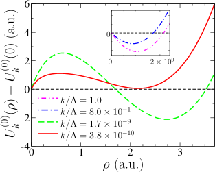
Figure 2: Gibbs free energy $U^{(0)}_{k}(\rho)$ vs $\rho$ for various values of $k$ and $\mu^{\prime}=\mu^{\prime}_{c}$. The potential exhibits a single minimum at the beginning of the RG flow (see inset) whereas 2 minima coexist for sufficiently small $k$.

For the numerical solution of the RG equations, we use the known values of $a_{0}$ and $a_{2}$ for the Bose gas of interest (e.g. ⁸⁷Rb) and choose a typical experimental value for the density $n$ [Wechooseavalueofthedensitycorrespondingtoarecentexperimentwheretheatomsweretrappedinaquasi-uniformpotential:]Gaunt13. We set the temperature equal to its critical value $T_{c}\simeq(2\pi/M)(n/3\zeta(3/2))^{2/3}$ not (f) and vary the chemical potential $\mu^{\prime}$ to locate the transition. When lengths are expressed in units of the thermal de Broglie wavelength $\lambda_{\rm dB}$, results are independent of the boson mass $M$.

Figure 2 shows the $k$-dependence of the effective potential $U_{k}^{(0)}(\rho)$ at the transition ($\mu^{\prime}=\mu^{\prime}_{c}$) for a ⁸⁷Rb atom gas. Initially, for $k=\Lambda$, the system is ordered and $U_{k}^{(0)}(\rho)$ shows a minimum at a nonzero value $\rho_{0,\Lambda}$. The effect of fluctuations is twofold. Long-range order is suppressed as $k$ decreases (i.e. $\rho_{0,k}$ decreases) and for sufficiently small $k$ a second minimum appears at $\rho=0$. Both minima become degenerate when $k\to 0$. For $\mu^{\prime}<\mu^{\prime}_{c}$, the minimum at $\rho=0$ is the absolute minimum (normal phase), whereas the nontrivial minimum is the absolute one when $\mu^{\prime}>\mu^{\prime}_{c}$ (superfluid phase). As a consequence the order parameter makes a discontinuous jump at the phase transition, which is therefore (fluctuation-induced) first order. The RG equation $\partial_{k}U_{k}$ is unstable for small $k$ so that it is not possible to determine the effective potential for arbitrary small values of $k$ not (g). Nevertheless, we find that all physical quantities (e.g. the location of the minima of $U_{k}^{(0)}(\rho)$ or the correlation length) have nearly converged before the instability occurs not (h), and the sole effect of continuing the flow (if it were possible) would be to make the inner part of the potential convex (as required by its definition as a Legendre transform).

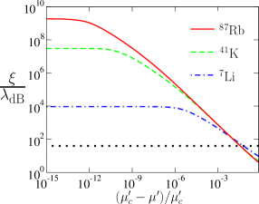
Figure 3: Correlation length $\xi$ vs renormalized chemical potential $\mu^{\prime}$. The pseudocritical exponent $\nu$ is defined by the slope of the linear dependence of $\ln(\xi/\lambda_{\rm dB})$ vs $\ln(\mu^{\prime}_{c}-\mu^{\prime})/\mu^{\prime}_{c}$. The horizontal dotted line shows the size of the system in a typical experiment.

Figure 3 shows the correlation length $\xi=(Z_{k=0}/U^{(0)}_{k=0}{}^{\prime}(0))^{1/2}$ deduced from the one-particle Green function ($Z_{k}$ denotes the wavefunction renormalization factor and the prime a $\rho$ derivative), obtained from the smallest reachable value of $k$ not (h), as a function of the renormalized chemical potential. For all atoms considered, ⁸⁷Rb, ⁴¹K and ⁷Li, $\xi$ is finite at the transition but several orders of magnitude larger than $\lambda_{\rm dB}$, i.e. much larger than the size $L$ of the system in a typical experiment. This implies that neither the finiteness of $\xi(\mu^{\prime}_{c})$ nor the jump $\Delta n_{0}$ of the condensate density can be observed experimentally (Table 1). However, as first pointed out in the context of the magnetic transition in STHAs Zumbach (1993), the strong increase of the correlation length as the transition is approached allows one to define a (nonuniversal) pseudocritical exponent $\nu$ by $\xi\sim(\mu^{\prime}_{c}-\mu^{\prime})^{-\nu}$ for $\xi\lesssim L$. Note that the same exponent $\nu$ characterizes the increase of the correlation length, i.e. $\xi\sim(T-T_{c})^{-\nu}$, if the transition is approached at fixed chemical potential by varying the temperature. Figure 3 shows that the regime where pseudoscaling holds is reached as soon as $\xi$ becomes equal to a few de Broglie wavelengths, which suggests that this regime can be observed on a significant temperature range.

Remarkably, the value of $\nu$ differs significantly for ⁸⁷Rb, ⁴¹K and ⁷Li and therefore provides us with a possible experimental test of the theory (Table 1). The value of $\nu$ varies by less than 2% if we include only $U_{k}^{(1)}(\rho)$ in (6) which shows that the field expansion is nearly converged. Furthermore, higher-order derivative terms not included in the LPA’ are expected to be essentially irrelevant for the computation of $\nu$ when, as is the case here, the anomalous dimension $\eta_{k}=-k\partial_{k}\ln Z_{k}$ is small. The estimate of $\nu$ is however sensitive to the precise value of the momentum cutoff $\Lambda\sim\lambda_{\rm dB}^{-1}$ (the only parameter which is not precisely known in our theory). For instance, varying $\Lambda$ between $0.25\lambda_{\rm dB}^{-1}$ and $4\lambda_{\rm dB}^{-1}$ one finds $0.55\leq\nu\leq 0.62$ for ⁷Li. An improved estimate could be obtained by including quantum fluctuations in the NPRG approach, thus removing the need to introduce a ultraviolet momentum cutoff. Nevertheless, the difference in the value of $\nu$ for ⁸⁷Rb, ⁴¹K and ⁷Li is clearly a robust prediction not (i).

Table 1: Correlation length $\xi(\mu^{\prime}_{c})$, condensate-density jump $\Delta n_{0}$ and pseudocritical exponent $\nu$. The values of $a_{0}$ and $a_{2}$ are taken from Ref. Stamper-Kurn and Ueda (2013). $a_{B}$ denotes the Bohr radius and $\lambda_{\rm dB}$ the thermal de Broglie wavelength.

	87Rb	41K	7Li
$a_{0}/a_{B}$	$101.8\pm 0.2$	$68.5\pm 0.7$	23.9
$a_{2}/a_{B}$	$100.4\pm 0.1$	$63.5\pm 0.6$	6.8
$\xi(\mu^{\prime}_{c})/\lambda_{\rm dB}$	$1.8\times 10^{9}$	$3.0\times 10^{7}$	$9.1\times 10^{3}$
$\Delta n_{0}\lambda^{3}_{\rm dB}$	$2.7\times 10^{-9}$	$1.9\times 10^{-7}$	$9.3\times 10^{-4}$
$\nu$	0.77	0.74	0.59

The difference between ⁸⁷Rb, ⁴¹K and ⁷Li is illustrated in the RG flow diagram of Fig. 4 showing the dimensionless coupling constants $\tilde{\lambda}_{1,k}=\lambda_{1}/(Z_{k}^{2}k)$ and $\tilde{\lambda}_{2,k}=\lambda_{2}/(Z_{k}^{2}k)$ as a function of the RG momentum scale $k$. In the case of ⁸⁷Rb, for which $\tilde{\lambda}_{2,\Lambda}$ is very small, the RG trajectory passes near the Wilson-Fisher fixed point of the O(6) model. The RG flow terminates when $k\sim 1/L$ and, for the typical system size $L$ considered, does not leave the region of influence of the O(6) Wilson-Fisher fixed point. It is therefore not a surprise that the pseudocritical exponent $\nu\simeq 0.77$ is not very different from the exponent $\nu_{\rm O(6)}\simeq 0.83$ of the O(6) model. The RG trajectory for ⁴¹K is also strongly attracted by the O(6) Wilson-Fisher fixed point. In the case of ⁷Li, pseudoscaling is due to the RG trajectory passing in the vicinity of an unphysical fixed point with complex coordinates and projection (0.690,3.110) in the plane $(\tilde{\lambda}_{1,k},\tilde{\lambda}_{2,k})$. In the O($N$)$\times$O(2) model with $N=5$, this unphysical fixed point slows down the RG trajectories and leads to pseudoscaling Delamotte et al. (2004); Zumbach (1993). For $N=4$ and $N=3$ no minimum in the velocity of the flow is obtained for ⁸⁷Rb, ⁴¹K and ⁷Li, but the RG trajectories in the neighborhood of the unphysical fixed point are nevertheless slow enough for pseudoscaling to be observable.

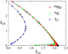
Figure 4: RG flow in the plane $(\tilde{\lambda}_{1,k},\tilde{\lambda}_{2,k})$. The solid symbols show the initial conditions of the trajectories. The black dot shows the Wilson-Fisher fixed point of the three-dimensional O(6) model.

Conclusion and experimental discussion. We have shown that the O(3)$\times$O(2) model describing the magnetic phase transition in STHAs can be simulated with spin-one Bose gases. The NPRG approach predicts weakly first-order transitions in STHAs and spin-one Bose gases with pseudoscaling without universality. Our predictions can be tested by determining experimentally the correlation length $\xi$ and the pseudocritical exponent $\nu$ using matter-wave interferometry Donner et al. (2007); Navon et al. (2015). The value of $\nu$ in ⁸⁷Rb and ⁴¹K atom gases, which is close to $\nu_{\rm O(6)}$, is largely a consequence of a crossover phenomenon due to the proximity of the O(6) Wilson-Fisher fixed point, and is independent of the ultimate first-order character of the transition. By contrast, the value $\nu\simeq 0.59$ in ⁷Li is not related in any way to the existence of a nearby critical fixed point: This value is nonuniversal and depends solely on the scattering lengths $a_{0}$ and $a_{2}$. Experimental confirmation of this result would therefore be a very strong indication that the weakly-first-order scenario predicted by NPRG is correct.

One could also consider varying the scattering lengths $a_{0}$ and $a_{2}$ by means of a Feshbach resonance. But the external magnetic field, which in general is used to adjust the resonance, would unfortunately suppress the O(3) spin-rotation symmetry. A way out of this difficulty could come from microwave-induced Feshbach resonances as proposed in Ref. Papoular et al. (2010). Modifying the scattering lengths in ⁷Li would allow a direct confirmation of pseudoscaling, i.e. that the value of $\nu$ changes with $a_{0}$ and $a_{2}$. Increasing $a_{0}$ by a factor of 4 (with $a_{2}$ fixed) would be sufficient to have $\xi(\mu^{\prime}_{c})<L$ and make the first-order character of the transition observable.

We would like to thank B. Delamotte, D. Mouhanna and M. Tissier for numerous discussions on the NPRG approach to frustrated magnets, and F. Gerbier and C. Salomon for enlightening discussions on spin-one Bose gases.

References

- Bloch et al. (2008) I. Bloch, J. Dalibard, and W. Zwerger, Rev. Mod. Phys. 80, 885 (2008).
- not (a) The sign (ferromagnetic or antiferromagnetic) of the coupling in the third direction does not matter since it does not introduce any frustration.
- Yosefin and Domany (1985) M. Yosefin and E. Domany, Phys. Rev. B 32, 1778 (1985).
- Kawamura (1988) H. Kawamura, Phys. Rev. B 38, 4916 (1988).
- Zinn-Justin (1996) J. Zinn-Justin, Quantum Field Theory and Critical Phenomena (Third Edition, Clarendon Press, Oxford, 1996).
- Delamotte et al. (2004) B. Delamotte, D. Mouhanna, and M. Tissier, Phys. Rev. B 69, 134413 (2004).
- Pelissetto et al. (2001) A. Pelissetto, P. Rossi, and E. Vicari, Phys. Rev. B 63, 140414 (2001).
- Calabrese et al. (2002) P. Calabrese, P. Parruccini, and A. I. Sokolov, Phys. Rev. B 66, 180403 (2002).
- Calabrese et al. (2003) P. Calabrese, P. Parruccini, and A. I. Sokolov, Phys. Rev. B 68, 094415 (2003).
- Calabrese et al. (2004) P. Calabrese, P. Parruccini, A. Pelissetto, and E. Vicari, Phys. Rev. B 70, 174439 (2004).
- not (b) A focus fixed point is defined by a stability matrix having complex eigenvalues.
- Delamotte et al. (2010) B. Delamotte, M. Dudka, Y. Holovatch, and D. Mouhanna, Phys. Rev. B 82, 104432 (2010).
- Nakayama and Ohtsuki (2015) Y. Nakayama and T. Ohtsuki, Phys. Rev. D 91, 021901 (2015).
- not (c) For a critical discussion of the conformal bootstrap program applied to the O(3)O(2) model, see Ref. Delamotte et al. (2016).
- Garel and Pfeuty (1976) T. Garel and P. Pfeuty, J. Phys. C 9, L245 (1976).
- Bailin et al. (1977) D. Bailin, A. Love, and M. A. Moore, J. Phys. C 10, 1159 (1977).
- Antonenko et al. (1995) S. Antonenko, A. Sokolov, and K. Varnashev, Phys. Lett. A 208, 161 (1995).
- Holovatch et al. (2004) Y. Holovatch, D. Ivaneyko, and B. Delamotte, J. Phys. A 37, 3569 (2004).
- Calabrese and Parruccini (2004) P. Calabrese and P. Parruccini, Nucl. Phys. B 679, 568 (2004).
- Tissier et al. (2000) M. Tissier, D. Mouhanna, and B. Delamotte, Phys. Rev. B 61, 15327 (2000).
- Tissier et al. (2003) M. Tissier, B. Delamotte, and D. Mouhanna, Phys. Rev. B 67, 134422 (2003).
- Delamotte et al. (2016) B. Delamotte, M. Dudka, D. Mouhanna, and S. Yabunaka, Phys. Rev. B 93, 064405 (2016).
- Zumbach (1993) G. Zumbach, Phys. Rev. Lett. 71, 2421 (1993).
- Delamotte et al. (2013) B. Delamotte, D. Mouhanna, and M. Tissier, in Frustrated spin systems, edited by H. T. Diep (World Scientific, Singapore, 2013) 2nd ed.
- Ohmi and Machida (1998) T. Ohmi and K. Machida, J. Phys. Soc. Jpn 67, 1822 (1998).
- Ho (1998) T.-L. Ho, Phys. Rev. Lett. 81, 742 (1998).
- Kawaguchi and Ueda (2012) Y. Kawaguchi and M. Ueda, Phys. Rep. 520, 253 (2012).
- Stamper-Kurn and Ueda (2013) D. M. Stamper-Kurn and M. Ueda, Rev. Mod. Phys. 85, 1191 (2013).
- Ceccarelli et al. (2015) G. Ceccarelli, J. Nespolo, A. Pelissetto, and E. Vicari, Phys. Rev. A 92, 043613 (2015).
- Berges et al. (2002) J. Berges, N. Tetradis, and C. Wetterich, Phys. Rep. 363, 223 (2002).
- Delamotte (2012) B. Delamotte, in Renormalization Group and Effective Field Theory Approaches to Many-Body Systems, Lecture Notes in Physics, Vol. 852, edited by A. Schwenk and J. Polonyi (Springer Berlin Heidelberg, 2012) pp. 49–132.
- Kopietz et al. (2010) P. Kopietz, L. Bartosch, and F. Schütz, Introduction to the Functional Renormalization Group (Springer, Berlin, 2010).
- Berges and Wetterich (1997) J. Berges and C. Wetterich, Nucl. Phys. B 487, 675 (1997).
- Fukushima et al. (2011) K. Fukushima, K. Kamikado, and B. Klein, Phys. Rev. D 83, 116005 (2011).
- Fejös (2014) G. Fejös, Phys. Rev. D 90, 096011 (2014).
- not (d) See also Ref. Delamotte et al. (2016).
- Gaunt et al. (2013) A. L. Gaunt, T. F. Schmidutz, I. Gotlibovych, R. P. Smith, and Z. Hadzibabic, Phys. Rev. Lett. 110, 200406 (2013).
- not (f) Here we use the noninteracting value of the transition temperature. For a dilute gas, corrections due to interactions are small (of order ).
- not (g) This instability is due to a pole appearing in the propagator at a finite value of the RG momentum scale , which prevents to continue the flow for .
- not (h) In practice, we extrapolate the results to in order to obtain high-precision values.
- not (i) In Ref. Natu and Mueller (2011) it has been predicted using a mean-field approximation that the (second-order) superfluid transition to the ferromagnetic phase becomes a ferromagnetic transition without Bose-Einstein condensation (BEC) when , which is the case in the 7Li atom gas. Discarding the first-order character of the superfluid transition discussed in this Rapid Communication, we expect fluctuations beyond mean field to increase the superfluid transition temperature but decrease the ferromagnetic transition temperature. Assuming that the shift of the BEC temperature is given by Arnold and Moore (2001) and using the mean-field results of Natu and Mueller (2011) for the transition temperature of the ferromagnetic transition (without BEC), we find that 7Li undergoes a superfluid transition rather than a ferromagnetic transition without BEC.
- Donner et al. (2007) T. Donner, S. Ritter, T. Bourdel, A. Öttl, M. Köhl, and T. Esslinger, Science 315, 1556 (2007).
- Navon et al. (2015) N. Navon, A. L. Gaunt, R. P. Smith, and Z. Hadzibabic, Science 347, 167 (2015).
- Papoular et al. (2010) D. J. Papoular, G. V. Shlyapnikov, and J. Dalibard, Phys. Rev. A 81, 041603 (2010).
- Natu and Mueller (2011) S. S. Natu and E. J. Mueller, Phys. Rev. A 84, 053625 (2011).
- Arnold and Moore (2001) P. Arnold and G. Moore, Phys. Rev. Lett. 87, 120401 (2001).