Abstract

We study theoretically how multiple scattering of light in a disordered medium can spontaneously generate quantum correlations. In particular we focus on the case where the input state is Gaussian and characterize the correlations between two arbitrary output modes. As there is not a single all-inclusive measure of correlation, we characterise the output correlations with three measures: intensity fluctuations, entanglement, and quantum discord. We found that, while a single mode coherent state input can not produce quantum correlations, any other Gaussian input will produce them in one form or another. This includes input states that are usually regarded as more classical than coherent ones, such as thermal states, which will produce a non zero quantum discord.

OCIS codes: (290.4210) Multiple scattering; (290.7050) Turbid media; (270.0270) Quantum optics.

1 Introduction

Light propagation in a scattering medium can often be described as a diffusive process [1], where any memory of the initial state is lost almost immediately, and transport is represented by the incoherent sum over many Brownian random walks. However it was early realized that temporal coherence survives multiple elastic scattering, and thus interference is still possible even after passing through a diffusive medium [2]. As a consequence of interference the diffusive picture has to be modified, and the light scattered into different channels develop correlations [3]. Classical correlations between the intensity scattered in one direction and the intensity scattered into another direction were studied since the ’60s [4, 5] and found many applications, especially in imaging, e.g. in dynamic light scattering [6], speckle contrast imaging [7], stellar speckle interferometry [8], wavefront shaping [9], and speckle scanning microscopy [10, 11]. The study of quantum correlations of multiply scattered light started much later, probably due to the widespread idea that quantum features are frail and thus unlikely to play a significant role in the presence of strong disorder. Nevertheless it was recently shown that not only certain quantum features can survive multiple scattering [12], but that quantum correlations can even be spontaneously created in the scattering process [13]. The quantum properties of scattered light proved to be so robust that control over the transport of single photons in a disordered medium via wavefront shaping was demonstrated [14, 15].

In this paper we consider the case of a generic Gaussian input state and study theoretically the necessary conditions for the output state to present quantum correlations. In particular we show that, while entanglement requires specific conditions to be produced, quantum discord is always present in the output state when a thermal input state is used but, surprisingly, not when the input mode is in a coherent state.

2 Quantum correlations between two modes

Classical correlations of scattered light are commonly described by a correlation function $\mathcal{C}_{l,m}$ that measures the correlations between intensity fluctuations of two different modes $l$ and $m$ [3, 4, 5],

$$\mathcal{C}_{l,m}=\frac{\left\langle I_{l}I_{m}\right\rangle}{\left\langle I_{l}\right\rangle\left\langle I_{m}\right\rangle},$$ (1)

where $I=\left|E\right|^{2}$ is the light intensity and $\left\langle\cdot\right\rangle$ represents either a time or an ensemble average (if the system is ergodic the two are equivalent). $\mathcal{C}$ can be used beyond the classical case to study certain classes of quantum correlations by substituting $I$ with the mode’s number operator $\hat{n}$ [16, 17], and since classical light can never lead to $\mathcal{C}<1$, a correlation value below 1 is considered a clear signature of quantumness [18].

In order to study the effect of multiple scattering on a Gaussian input state we employ the formalism of density operators and covariance matrices [19]. The covariance matrix of two output modes is defined as

$$\sigma_{\mu,\nu}=\frac{1}{2}\langle\hat{R}_{\mu}\hat{R}_{\nu}+\hat{R}_{\nu}\hat{R}_{\mu}\rangle-\langle\hat{R}_{\mu}\rangle\langle\hat{R}_{\nu}\rangle,\quad\mu,\nu=1,...,2N,$$ (2)

where $\hat{R}=\{\hat{x}_{1},\hat{p}_{1}\dots\hat{x}_{N},\hat{p}_{N}\}$ is the vector of quadrature operators, that satisfies the commutation relation $[\hat{R}_{\mu},\hat{R}_{\nu}]=i\,\left(\Omega^{\oplus N}\right)_{\mu,\nu}$, which imposes constrains on $\sigma$:

$$\sigma+i\Omega^{\oplus N}\geq 0\quad\mbox{with}\quad\Omega=\begin{pmatrix}0&1\\ -1&0\end{pmatrix},$$ (3)

where $\oplus$ is a direct sum. Importantly, for Gaussian states the covariance matrix captures all the correlation properties between the modes. As will be discussed below, different measures of quantum correlations, such as entanglement and discord, can be formulated as conditions on the elements of the covariance matrix.

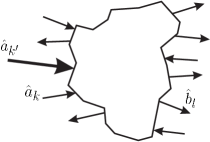
Fig. 1: The disordered medium is scattering $N$ input modes $\hat{a}_{k}$ into $N$ output modes $\hat{b}_{l}$. The scattering process is described by a scattering matrix $S$. The only non-empty input mode is $\hat{a}_{k^{\prime}}$, the others are assumed to be in a vacuum state.

When monochromatic light propagates through a disordered medium it is multiply scattered, and its wavefront becomes completely irregular. As a result the output modes take the form of a speckle pattern [2]. Here we consider a model of linear scattering, such that light propagation can be described by the scattering matrix $S$ [20], which couples the fields of the $N$ output modes, $E^{out}_{l}$, with the $N$ input modes, $E^{in}_{k}$ [17]. The electromagnetic field of a mode with polarization $\mathbf{e}_{k}$, wave vector $\mathbf{q}_{k}$ and frequency $\omega_{k}$ can be expressed as:

$$E^{in}_{k}(\mathbf{r})=\mathbf{e}_{k}\sqrt{\frac{2\hbar\omega_{k}}{2\epsilon_{0}V}}\left[\hat{a}_{k}e^{-i\mathbf{q}_{k}\mathbf{r}}+\hat{a}^{\dagger}_{k}e^{i\mathbf{q}_{k}\mathbf{r}}\right],$$ (4)

where $\hat{a_{k}}$ and $\hat{a}_{k}^{\dagger}$ are the creation and annihilation operators of the input mode, $\epsilon_{0}$ is the vacuum permittivity and $V$ is the mode volume [18]. The scattering matrix $S$ links the input fields to the output ones as $E^{out}_{l}=\sum_{k}^{N}S_{l,\,k}\,E^{in}_{k}$. Likewise for the ladder operators we have:

$$\hat{b}_{l}=\sum_{k}^{N}S_{l,k}\,\hat{a}_{k},\quad k,l,m=1..N.$$ (5)

Here $\hat{a}$ and $\hat{b}$ are the annihilation operators related to, respectively, the input and the output modes as shown in Fig. 1. The elements of the $S$ matrix are the complex transmission coefficients from the $k$-th input mode to the $l$-th output mode.

In this paper we focus on the correlations between two of the $N$ scattered modes, whose covariance matrix $\sigma$ has the structure:

$$\sigma=\begin{pmatrix}A&\Gamma\\ \Gamma^{T}&B\end{pmatrix},$$ (6)

where $A$, $B$, and $\Gamma$ are $2\times 2$ matrices. The matrices $A$ and $B$ refer to individual properties of the two modes, and the matrix $\Gamma$ describes the correlations between them. The determinants of these matrices, together with the determinant of the whole covariance matrix, are invariant under local transformations (i.e. those acting only on one of the modes). Because of this local invariance the determinants characterize entanglement and other non-local correlation properties of the state [21, 22, 23, 24]. Such two-mode covariance matrix can be written in the form

$$\sigma=\begin{pmatrix}\alpha&0&\gamma_{x}&0\\ 0&\alpha&0&\gamma_{p}\\ \gamma_{x}&0&\beta&0\\ 0&\gamma_{p}&0&\beta\end{pmatrix}$$ (7)

keeping the invariants of the state: $\det(A)=\alpha^{2},\,\det(B)=\beta^{2},\,\det(\Gamma)=\gamma_{x}\gamma_{p}$ and $\det(\sigma)$ the same [25].

The intensity correlation $\mathcal{C}$ contains fourth order moments of the field distribution. For Gaussian states these can always be written as a function of the second order moments, contained in the covariance matrix $\sigma$ [19]. This leads to the expression for the correlation function:

$$\mathcal{C}=1+\frac{(2\gamma_{x}^{2}+2\gamma_{p}^{2})}{(2\alpha-1)(2\beta-1)}.$$ (8)

From Eq. (8) we can see that Gaussian states always have $\mathcal{C}\geq 1$, as $\alpha,\beta\geq 1/2$ as a consequence of the commutation relations in Eq. (3).

While $\mathcal{C}$ is useful to describe classical correlations and certain features of quantum light, like photon anti-bunching [16], it does not capture other quantum correlations, and thus other measures have been introduced, notably entanglement and discord. The characterization of entanglement for general mixed states of multiple modes is a challenging task. Necessary and sufficient conditions for entanglement have been identified for bipartite discrete quantum systems of $2\times 2$ and $2\times 3$ dimensions [22, 23] and for continuous two-mode Gaussian states [25, 26]. In the latter case, these mathematical conditions can be understood as inverting time in one of the modes of the system and checking if the resulting quantum state is still a valid physical state, i.e. hermitian and positive [22, 23, 25, 26]. These conditions on the quantum state can be recast as conditions on the matrix $\sigma^{\prime}$, obtained from the covariance matrix $\sigma$ Eq. (7), by changing the sign to the momentum of one of the two modes, i.e. $\sigma^{\prime}=\sigma(\gamma_{p}\to-\gamma_{p})$. If $\sigma^{\prime}$ obeys the commutation relation stated in Eq. (3) then the two modes are separable, otherwise they are entangled. This separability condition for the two modes can be rewritten as [21],

$$\eta^{\pm}:=\left[\frac{1}{2}\left(\Delta^{\prime}\pm\sqrt{\Delta^{\prime 2}-4\det(\sigma^{\prime})}\right)\right]^{1/2}\geq 1/2,$$ (9)

where $\Delta^{\prime}=\det(A)+\det(B)+2\det(\Gamma^{\prime})$ refers to the sub-matrices of the covariance matrix $\sigma^{\prime}$ and $\det(\Gamma^{\prime})=-\gamma_{p}\gamma_{x}$ (see Eq. (6) and Eq. (7)). $\eta^{\pm}$ are the symplectic eigenvalues of the matrix $\sigma^{\prime}$ [19].

When the parameters $\alpha$ and $\beta$ (i.e. the number of photons in each of the modes) are fixed, Eq. (3) and Eq. (9) define closed regions in the $\gamma_{x}$ and $\gamma_{p}$ parameter space (see Fig. 2). The condition in Eq. (3) defines an area enclosed by the thick solid line in Fig. 2, which corresponds to all valid states. The entangled states lie within this areas but outside the region defined by the condition in Eq. (9) (gray areas in Fig. 2), which can be graphically obtained as the first region rotated by $90^{\circ}$ (dotted lines in Fig. 2).

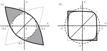
Fig. 2: Map of all possible two-mode Gaussian states and their correlations, as a function of the off-diagonal elements $\gamma_{x}$ and $\gamma_{p}$ of the covariance matrix in Eq. (7), with diagonal values $\alpha$ and $\beta$: (a) $\alpha=\beta=0.75$, (b) $\alpha=\beta=5$. All physically allowed states lie within the region enclosed by the thick solid line. The region of separable states can be found as the intersection of the allowed state region and its mirror image with respect of $\gamma_{p}$ (dotted line) [25]. The remaining states (in the gray area) are not separable, i.e. they are entangled. For a thermal input state the output states, Eq. (15), lie on the $\gamma_{x}=\gamma_{p}$ line, and thus are not entangled. The dashed circle corresponds to the condition $\mathcal{C}=2$. Inside this circle $\mathcal{C}$ is less than 2, with $\mathcal{C}=1$ at the origin. Increasing the number of photons in the input state, i.e. increasing $\alpha$ and $\beta$, the fraction of entangled output states decreases and some entangled states cross into the $\mathcal{C}=2$ circle, as shown in panel (b).

For a long time entanglement was considered to be the quintessential non-classical ingredient for quantum computation and communication. However, it was shown that even using separable (i.e. non-entangled) states it is possible to perform certain computational tasks exponentially faster than any known classical algorithm [27]. This means that just the fact of the system being quantum may lead to applications impossible for classical systems, irrespectively of separability. This fact has been formalized by introducing quantum discord [28], a measure which broadens the concept of non-classical correlations to states without entanglement.

For a pure bipartite entangled state the measurement of one of the parties completely determines the result of the measurement on the second, while for classical states measurement on one party does not effect the other. On the other hand there are separable states where the measurement of one party influences the other in a probabilistic sense [29, 30], making them non-classical, but not entangled either. Quantum discord quantifies this influence and is defined as the discrepancy of two measures of mutual information for a joint quantum state $\rho_{AB}$ of systems $A$ and $B$:

$$I^{q}(\rho_{AB})=S(\rho_{A})+S(\rho_{B})-S(\rho_{AB})\quad\text{and}\quad J^{q}(\rho_{AB})=S(\rho_{A})-\sum_{j}Tr[\rho_{AB}\Pi_{j}]\,\,S(\rho_{A|\Pi_{j}}).$$ (10)

Here $\rho_{A}=Tr_{B}[\rho_{AB}]$ and $\rho_{B}=Tr_{A}[\rho_{AB}]$ are the reduced states of $\rho_{AB}$ and $S$ is the von Neumann entropy: $S(\rho)=-Tr[\rho\ln\rho]$. The second equation depends on the measurement choice $\{\Pi_{j}\}$, and $\rho_{A|\Pi_{j}}=Tr_{B}[\rho_{AB}\Pi_{j}]/Tr[\rho_{AB}\Pi_{j}]$ is the state of the system A conditioned on a certain outcome of this measurement performed on the subsystem B.

Quantum discord $D(\rho_{AB})$ is quantified by the difference between the two expressions in Eq. (10) minimized over all possible sets of measurement operators,

$$D(\rho_{A|B})=\inf_{\Pi_{j}}\left(I^{q}(\rho_{AB})-J^{q}(\rho_{AB})\right)=S(\rho_{B})-S(\rho_{AB})+\inf_{\Pi_{j}}\sum_{j}Tr[\rho_{AB}\Pi_{j}]\,S(\rho_{A|\Pi_{j}}).$$ (11)

When the input state is Gaussian and its covariance matrix is $\sigma$, the expression for the entropy of this state reduces to: $S(\sigma)=\sum_{i}\kappa(\eta_{i})$, where $\eta_{i}$ are the symplectic eigenvalues of $\sigma$ and $\kappa(z)=(z+1/2)\ln(z+1/2)+(z-1/2)\ln(z-1/2)$ [31]. Here we limit ourselves to Gaussian measurements, i.e. those that preserve the Gaussian nature of the state they are applied to. Under this assumptions the minimization of Eq. (11), written as a function of the invariants of the covariance matrix $\sigma$ from Eq. (7), gives:

$$D_{G}(\sigma)=\kappa(\sqrt{\det(B)})-\kappa(\eta^{-})-\kappa(\eta^{+})+\kappa\left(\frac{\sqrt{\det(A)}+2\sqrt{\det(A)\det(B)}+2\det(\Gamma)}{1+2\sqrt{\det(B)}}\right),$$ (12)

which is known as Gaussian discord [32]. The Gaussian discord $D_{G}$ vanishes if and only if $\Gamma=0$ [21, 29, 32].

3 Correlations between two scattered modes

To characterize the correlation of two modes of the scattered light we explicitly calculate the elements of the corresponding covariance matrix. We will consider the experimentally common situation where the input light is in a single mode $k^{\prime}$, and all the other input modes are in a vacuum state, as depicted in Fig. 1. Replacing the quadrature operators in the vector $\hat{R}$ with the ladder operators: $\hat{x}=(\hat{b}+\hat{b}^{\dagger})/\sqrt{2}$ and $\hat{p}=(\hat{b}-\hat{b}^{\dagger})/i\sqrt{2}$, and substituting Eq. (5) in, the general expression for the elements of the covariance matrix of two output modes is

$$\sigma_{2l-1,2m-1} =\frac{\delta_{l,m}}{2}+W_{l,m}\,\Delta\hat{n}_{k^{\prime}}+Y_{l,m}\,\Delta\hat{a}_{k^{\prime}}\hat{a}_{k^{\prime}}+Y^{*}_{l,m}\,\Delta\hat{a}_{k^{\prime}}^{\dagger}\hat{a}_{k^{\prime}}^{\dagger},$$ (13)

$$\sigma_{2l,2m} =\frac{\delta_{l,m}}{2}+W_{l,m}\,\Delta\hat{n}_{k^{\prime}}-Y_{l,m}\,\Delta\hat{a}_{k^{\prime}}\hat{a}_{k^{\prime}}-Y^{*}_{l,m}\,\Delta\hat{a}_{k^{\prime}}^{\dagger}\hat{a}_{k^{\prime}}^{\dagger},$$

$$\sigma_{2l-1,2m}=\sigma_{2l,2m-1} =\frac{1}{2i}\big{[}Z_{l,m}\,\Delta\hat{n}_{k^{\prime}}+Y_{l,m}\,\Delta\hat{a}_{k^{\prime}}\hat{a}_{k^{\prime}}-Y^{*}_{l,m}\,\Delta\hat{a}_{k^{\prime}}^{\dagger}\hat{a}_{k^{\prime}}^{\dagger}\big{]},$$

where

$$\Delta\hat{n}_{k^{\prime}} =\langle\hat{a}^{\dagger}_{k^{\prime}}\hat{a}_{k^{\prime}}\rangle-\langle\hat{a}^{\dagger}_{k^{\prime}}\rangle\langle\hat{a}_{k^{\prime}}\rangle,$$

$$\Delta\hat{a}_{k^{\prime}}\hat{a}_{k^{\prime}} =\langle\hat{a}_{k^{\prime}}\hat{a}_{k^{\prime}}\rangle-\langle\hat{a}_{k^{\prime}}\rangle\langle\hat{a}_{k^{\prime}}\rangle$$

$$W_{l,m} =\left(S^{*}_{l,k^{\prime}}S_{m,k^{\prime}}+S^{*}_{m,k^{\prime}}S_{l,k^{\prime}}\right),$$

$$Z_{l,m} =\left(S^{*}_{l,k^{\prime}}S_{m,k^{\prime}}-S^{*}_{m,k^{\prime}}S_{l,k^{\prime}}\right),$$

$$Y_{l,m} =S_{l,k^{\prime}}S_{m,k^{\prime}},$$

This expression allows us to analyse the correlation properties between two output modes, e.g. entanglement and quantum discord, for different possible inputs.

Coherent state:

If the input mode is in a coherent state Eq. (8) gives the value of $\mathcal{C}_{l,m}=1$ as expected, which means that there is no correlation between the intensity fluctuations of the two output modes according to this measure [33]. Since all expectation values of the operators $\Delta\hat{n}_{k^{\prime}}$ and $\Delta\hat{a}_{k^{\prime}}\hat{a}_{k^{\prime}}$ are 0, the covariance matrix of the output modes will be $\sigma^{coh}=\frac{1}{2}\mathbb{1}$. Substituting the elements of $\sigma^{coh}$ into Eq. (9), the allowed region shrinks to a point $\gamma_{x}=~{}\gamma_{p}=0$. This means that for any coherent state as an input, any two output modes will simply be a product of two coherent states and no quantum correlations are present.

Squeezed state:

If the input mode is in a squeezed state with a squeezing parameter $r$ and phase $\theta$, the expectation values for the operators in Eq. (13) are: $\Delta\hat{a}_{k^{\prime}}\hat{a}_{k^{\prime}}=-e^{i\theta}\sinh(r)\cosh(r)$, and $\Delta\hat{n}_{k^{\prime}}=\sinh^{2}(r)$ [34]. If we set $\theta=0$, for which we expect maximal entanglement [19], we can express the entanglement criterion as $\sinh(r)^{2}|S_{l,k^{\prime}}|^{2}|S_{m,k^{\prime}}|^{2}>0$, which is always true if $r$ and both scattering matrix elements are non-zero. This means that we will get entanglement for any non-zero degree of squeezing $r$ [35]. It is remarkable that the degree of entanglement does not depend on the phases of transmission coefficients of the scattering matrix, but only on their moduli.

Although quantum features of intensity fluctuation correlations are often linked to $\mathcal{C}<1$, implying a reduction of coincidences in simultaneous detections of photons in the two modes, for squeezed states entanglement leads to positive correlation, which can lead to high $\mathcal{C}$. The maximal possible value of $\mathcal{C}$ which could be achieved with squeezed entangled states (the top left or bottom right points of the region of allowed states in Fig. 2) is:

$$\mathcal{C}^{sq}_{l,m}=2+\frac{|S_{l,k^{\prime}}|^{2}+|S_{m,k^{\prime}}|^{2}}{2\bar{n}|S_{l,k^{\prime}}||S_{m,k^{\prime}}|},$$ (14)

where $\bar{n}$ is the average number of photons in the input mode. When $\bar{n}\to\infty$, $\mathcal{C}^{sq}$ approaches 2, which corresponds to the value expected for thermal states. The presence of entanglement allows to reach values of $\mathcal{C}$ inaccessible for thermal states, and this is exploited in quantum imaging where it can allow faster recovery of information, especially in the low photon number regime [36]. However, this needs to be treated with some care. In fact, as it can be seen from Fig. 2b, with the increase of $\alpha$ and $\beta$ the circle $\mathcal{C}=2$ and the boundary of the gray area (corresponding to the entangled states) cross, and therefore it is possible to find non-entangled states with higher intensity correlations than some entangled states.

Thermal state:

For a thermal state $\rho_{th}$ we have: $Tr(\hat{a}_{k^{\prime}}\rho_{th})=Tr(\hat{a}_{k^{\prime}}^{\dagger}\rho_{th})=Tr(\hat{a}_{k^{\prime}}\hat{a}_{k^{\prime}}\rho_{th})=Tr(\hat{a}_{k^{\prime}}^{\dagger}\hat{a}_{k^{\prime}}^{\dagger}\rho_{th})=0$ and $Tr(\hat{a}_{k^{\prime}}^{\dagger}\hat{a}_{k^{\prime}}\rho_{th})=\bar{n}$. Using Eq. (13) the covariance matrix of the two output modes $l$ and $m$ can be written as:

$$\sigma^{th}_{l,m}=\begin{pmatrix}\sigma^{th}_{\alpha}&0&\sigma^{th}_{\gamma}&0\\[4.0pt] 0&\sigma^{th}_{\alpha}&0&\sigma^{th}_{\gamma}\\[4.0pt] \sigma^{th}_{\gamma}&0&\sigma^{th}_{\beta}&0\\[4.0pt] 0&\sigma^{th}_{\gamma}&0&\sigma^{th}_{\beta}\end{pmatrix}$$ (15)

with $\sigma^{th}_{\alpha}=|S_{l,k^{\prime}}|^{2}\bar{n}+\frac{1}{2}$, $\sigma^{th}_{\beta}=|S_{m,k^{\prime}}|^{2}\bar{n}+\frac{1}{2}$, and $\sigma^{th}_{\gamma}=\bar{n}|S_{l,k^{\prime}}||S_{m,k^{\prime}}|$.

The values of $\gamma_{x}$ and $\gamma_{p}$ in this case are equal. In Fig. 2 all possible thermal states lie on the line $\gamma_{x}=\gamma_{p}$ and thus no entanglement is possible according to the criterion described in Eq. (9). In fact, in order for the modes to be entangled, $\gamma_{x}$ and $\gamma_{p}$ should at least have different signs [25]. Although these states do not show entanglement, there are still quantum correlations between the output modes in the form of quantum discord.

We calculated the discord of the output covariance matrix for the case of input mode in the thermal state by substituting the output covariance matrix Eq. (15) into the formula for the Gaussian discord in Eq. (12). In Fig. 3 we plot the dependence of the Gaussian discord $D_{G}$ on the absolute values of the transmission coefficients from the mode $k^{\prime}$ to the modes $l$ and $m$. Notice that the discord $D$ is asymmetric against these coefficients since the measurement is performed on only one of the modes (on the mode $l$ in the Fig. 3). The discord increases monotonously with $|S_{l,k^{\prime}}|$, but there can be a maximum in its dependence on $|S_{m,k^{\prime}}|$, the position of which is defined by the number of photons in the input mode (Fig. 3b). At low photon numbers there is no maximum, and in that case the discord increases monotonously (Fig. 3a).

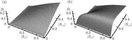
Fig. 3: The dependence of the Gaussian discord, $D_{G}$, between modes $l$ and $m$ on the absolute values of the elements of the scattering matrix $|S_{l,k^{\prime}}|$ and $|S_{m,k^{\prime}}|$. The input mode, $k^{\prime}$, is in a thermal state with different average photon numbers (a) $\bar{n}=1$, (b) $\bar{n}=10^{3}$. The measurement is performed on the mode $l$.

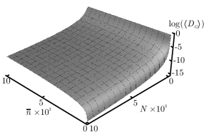
Fig. 4: Dependence of the average Gaussian discord, $\langle D_{G}\rangle$, on the number of output modes, $N$, and the number of photons, $\bar{n}$, in the thermal input state.

The mean discord obtained can be calculated noticing that, on average, the energy distributes equally among all the possible scattering channels and thus $\left\langle|S|^{2}\right\rangle=1/N$. If we assume that the scattered light follows a Rayleigh distribution we have $\left\langle|S|^{2}\right\rangle=2\left\langle|S|\right\rangle$ [3], which can be substituted into Eq. (12) to get the average amount of discord in a pair of output modes in this configuration. As shown in Fig. 4, $\left\langle D_{G}\right\rangle$ increases monotonically with $\bar{n}$, but decreases monotonically with $N$. As a consequence the best conditions to observe the discord generated by multiple scattering of a thermal state of light are obtained for an intense light signal scattering over a system with a small number of channels. Therefore we suggest that light scattering from systems showing Anderson localization [1, 3] will show a significant amount of quantum discord.

4 Conclusions

The search for a universal criterion that captures all the nuances of non-classical correlations is an object of ongoing intensive discussion [38, 39]. The presented results contribute to this debate by providing an illustration of the differences between various measures of quantum correlations, such as the correlation function based on intensity fluctuations $\mathcal{C}$, entanglement and discord. We calculated the covariance matrix of two arbitrary output modes of the light elastically scattered by a disordered material for different states of the input mode, and analysed their correlation properties. Surprisingly, the results show that if the input is a thermal state then any two output modes will be (Gaussian) discorded, a signature of the quantum character of light. Moreover, it turns out that coherent states are the only Gaussian input that do not produce quantum correlations, as measured by any of the quantities considered here.

It is known that the propagation of light through a scattering medium is modified by quantum interference when the input state is entangled [37], but the effects of quantum discord on light propagation are still a largely unexplored subject. Quantum discord appears naturally from the multiple scattering of thermal light, even for large photon numbers. Such macroscopic effects can potentially be exploited to develop novel imaging techniques. Since the amount of expected quantum discord grows when the number of scattering channels is small, these effects will play a role especially in the case of strongly scattering materials, where the dimensionless conductance $g$ is small [3]. In particular we expect it to have an effect for systems that show Anderson localization.

Finally, when light undergoes multiple scattering, even very weak nonlinearities can have a dramatic effect [40]. Thus diffusion through a nonlinear system will produce a very rich landscape of possible output states, opening the possibility to generate multimode entanglement from classical input light.

5 Acknowledgements

We are grateful to M. Paternostro, D. Browne, and M. Williamson for insightful discussions. JA acknowledges support by EPSRC (EP/M009165/1). JB acknowledges support from the Leverhulme Trust’s Philip Leverhulme Prize. IS acknowledges support from EPSRC through the Centre of Doctoral Training in Metamaterials ($\text{XM}^{2}$).