Numerical solution of the stationary multicomponent nonlinear Schrödinger equation with a constraint on the angular momentum

Abstract

We formulate a damped oscillating particle method to solve the stationary nonlinear Schrödinger equation (NLSE). The ground state solutions are found by a converging damped oscillating evolution equation that can be discretized with symplectic numerical techniques. The method is demonstrated for three different cases: for the single-component NLSE with an attractive self-interaction, for the single-component NLSE with a repulsive self interaction and a constraint on the angular momentum, and for the two-component NLSE with a constraint on the total angular momentum. We reproduce the so called yrast curve for the single-component case, described in [A. D. Jackson et al., Europhys. Lett. 95, 30002 (2011)], and produce for the first time an analogous curve for the two-component NLSE. The numerical results are compared with analytic solutions and competing numerical methods. Our method is well suited to handle a large class of equations and can easily be adapted to further constraints and components.

I Introduction

The nonlinear Schrödinger equation (NLSE) is important in many different fields of physics Fibich (2015): for example, in nonlinear optics Abdullaev et al. (2011); in superconductivity that can be modeled with the related Ginzburg-Landau equation Ögren et al. (2012); in vortex line models for dual strings in research in gravitation Nielsen and Olesen (1973); and self-gravitating models for dark matter Chavanis (2011). Here we present examples of NLSEs in the settings of a mean-field description of bosonic atoms, which has been an active area of research since the experimental breakthrough in the mid-1990s when Bose-Einstein condensates (BECs) were created in the laboratory with ultracold atomic gases Andersen et al. (1995); Bradley et al. (1995); Davis et al. (1995); Ensher et al. (1996). In this context the stationary NLSE typically has the form of a Gross-Pitaevskii equation

$$-\frac{\hbar^{2}}{2M}\nabla^{2}\varphi+U_{0}\left|\varphi\right|^{2}\varphi=\mu\varphi,$$ (1)

which is constrained by the normalization condition $\int\left|\varphi\right|^{2}\mathrm{d}V=N_{\varphi}$, where $N_{\varphi}$ is the number of atoms, M is the mass of an atom, and the atom-atom mean-field interaction parameter $U_{0}$ can be varied in sign and amplitude, for example, by an external magnetic field.

After the experimental achievements of creating BECs in the laboratory, numerical modeling of various properties of condensates accelerated. For example different techniques to solve Eq. (1) Dalfovo et al. (1996); Bao et al. (2006); Mallory and Van Gorder (2015); Mocz and Succi (2015), as well as for the corresponding time dependent equation Taha and Ablowitz (1984) have been developed. For modeling BEC dynamics it is crucial to maintain the normalization condition; see, e.g., Cerimele et al. (2000a, b) for methods that fulfill this to machine precision in each time step.

Furthermore, methods using a quantum lattice Boltzmann equation have been proposed to model expanding condensates Palpacelli and Succi (2008) over long times. More recently a connection between the Kohn-Sham equations, that can be used in density functional theory of bosonic as well as fermionic many-body systems and kinetic equations often occurring in modeling classical flows, have been developed Mendoza et al. (2014).

Also when solving for a stationary solution it is common to use a time-dependent equation Ruprecht et al. (1995) including dissipative damping, or to rewrite the evolution in an unphysical so-called imaginary time; see, e.g., Chin and Krotscheck (2005). In this work we will extend this idea by introducing a second-order derivative using an unphysical time parameter.

In this article we present a new versatile method for solving (1) and other nonlinear equations numerically. The method can be used for systems with extra constraints and more complex nonlinearities. Generalizations of (1), e.g., with two coupled components Mueller and Ho (2002), and even with different types of nonlinearities, as, e.g. quartic for modeling Fermi-Bose mixtures Abdullaev et al. (2013) can also be solved with the method presented here.

I.1 The dynamical functional particle method

Let us start quite general and assume that $\mathcal{F}$ is an operator, $v=v(x),\,v:X\rightarrow\mathbb{R}^{k},\,k\in\mathbb{N}$, and consider the abstract equation

$$\mathcal{F}(v)=0.$$ (2)

In this paper Eq. (2) will be the nonlinear Schrödinger equation. Further, introduce a parameter $\tau$ that belongs to some (unbounded) interval $T=[0,t_{1}],\,t_{1}\leq\infty$ and define a new equation in $u=u(x,\tau),\,u:X\times T\rightarrow\mathbb{R}^{k}$ as

$$\mathcal{M}u_{\tau\tau}+\eta u_{\tau}=\mathcal{F}(u),$$ (3)

where $\mathcal{M}=\mathcal{M}(x,u(x,t),t),\eta=\eta(x,u(x,t),t)$ are parameters. From physics we recognize (3) as a second-order damped system where $\mathcal{M}$ represents mass and $\eta$ the damping. Together with the two initial conditions on $u$ we will use (3) in such a way that $u_{t},\,u_{tt}\rightarrow 0$ when $t\rightarrow t_{1}$, i.e., $\lim_{t\rightarrow t_{1}}u(x,t)=v(x).$ In other words, we will solve the damped system (3) in order to attain the stationary solution $v(x).$ For simplicity we use $\mathcal{M}=1$ and $\eta$ constant (chosen to get fast convergence of the dynamical system).

We call the approach for solving (2) using (3) the dynamical functional particle method (DFPM) Edvardsson et al. (2012).

I.2 The model under study

As a first example we consider the NLSE (1) with an attractive interaction parameter, corresponding to $U_{0}<0$, on a ring with radius R. Such systems can model strongly confined BECs in axially symmetric traps studied experimentally, see e.g. Gupta et al. (2005). This system has a known analytic solution, described in detail in Appendix A, which will be used as a reference to the numerical solution.

We use the domain $-\pi R\leq x<\pi R$ with periodic boundary conditions and introduce the dimensionless angle coordinate $\Theta=x/R$. We divide all terms in (1) with $\hbar^{2}/\left(2MR^{2}\right)$ and insert a wave function $\Psi=\varphi/\sqrt{N_{\varphi}}$ normalized to unity. We can then introduce a dimensionless coupling constant $\gamma=N_{\varphi}MRU_{0}/\left(\pi\hbar^{2}\right)$, such that we obtain the normalized equation

$$-\frac{\partial^{2}\Psi}{\partial\Theta^{2}}+2\pi\gamma\left|\Psi\right|^{2}\Psi=\mu\Psi,$$ (4)

where $\mu$ is now a dimensionless eigenvalue. The energy functional corresponding to (4) is

$$E[\Psi]=\int_{-\pi}^{\pi}\left(\left|\frac{\partial\Psi}{\partial\Theta}\right|^{2}+\gamma\pi\left|\Psi\right|^{4}\right)\mathrm{d}\Theta,$$ (5)

subject to the normalization constraint

$$g_{1}[\Psi]:=\int_{-\pi}^{\pi}\left|\Psi\right|^{2}\mathrm{d}\Theta-1=0.$$ (6)

Equation (4) is obtained from the first variation of the constrained energy functional

$$E_{\mu}[\Psi]=E[\Psi]-\mu g_{1}[\Psi],$$ (7)

with respect to $\overline{\Psi}$. Variation with respect to $\mu$ gives Eq. (6).

Applying the DFPM (3) to (7), keeping the normalization constraint, gives the damped oscillating system

$$\frac{\partial^{2}\Psi}{\partial\tau^{2}}+\eta\frac{\partial\Psi}{\partial\tau}=\frac{\partial^{2}\Psi}{\partial\Theta^{2}}-2\pi\gamma\left|\Psi\right|^{2}\Psi+\mu\Psi,$$ (8)

where, as before, $\eta$ is the damping constant and $\tau$ is a dimensionless time parameter. Note that this equation is not the time-dependent NLSE. It is an unphysical equation that is constructed to have a solution that converges to a solution of the time-independent NLSE (4). The original functional (7) is a potential for a damped oscillating system whose stationary state is the solution of the NLSE (4).

II Numerics, Convergence and Accuracy

In order to solve (8) numerically we discretize in space and use a numerical method for the resulting system of ordinary differential equations. However, we first rewrite the Eq. (8) as a first-order system where we define the variables $q:=\Psi$ and $p:=\partial\Psi/\partial\tau$. We then have the dynamical system,

$$\dot{q}= p,$$ (9)

$$\dot{p}= \frac{\partial^{2}q}{\partial\Theta^{2}}-2\pi\gamma\left|q\right|^{2}q+\mu q-\eta p.$$

The unknown eigenvalue $\mu$ can be replaced by the integral $\mu=\int\overline{q}\left(-\frac{\partial^{2}q}{\partial\Theta^{2}}+2\pi\gamma\left|q\right|^{2}q\right)\mathrm{d}\Theta$, as can be seen by multiplying Eq. (4) with $\overline{\Psi}$, integrating over the domain and using the constraint (6).

Let $\left\{x^{i}\right\}_{i=1}^{N}=\left\{-\pi,\>-\pi+h,\ldots\pi-h\right\}$, be a partition of the interval $[-\pi,\pi)$ in $N$ points, where $h=2\pi/N$, and let $q_{n}^{i},\>p_{n}^{i}$ represent the values of $q,\>p$ at the point $x^{i}$ at some time $\tau_{n}=n\vartriangle\!\tau$. We modify the leapfrog method Hairer et al. (2006) to the damped oscillating system (8)

$$p_{n+1/2}^{i}= p_{n-1/2}^{i}+\vartriangle\!\!\tau\>(F[q_{n}^{i}]+\mu_{n}q^{i}_{n}-\eta\>p_{n-1/2}^{i}),$$ (10)

$$q_{n+1}^{i}= q_{n}^{i}+\vartriangle\!\!\tau\ p_{n+1/2}^{i},$$

where

$$F[q_{n}^{i}]=\dfrac{N}{4\pi}\left(q_{n}^{i+1}-2q_{n}^{i}+q_{n}^{i-1}\right)-2\pi\gamma\left|q_{n}^{i}\right|^{2}q_{n}^{i},$$ (11)

and $\mu_{n}$ is calculated with the trapezoidal approximation of the integral. The unit norm (6) is maintained by normalization of ${q_{n}^{i}}$ at each time step.

We can measure the convergence of the numerical method to the known analytic solution of the continuous problem (32), sampled at the $N$ grid points, in the Euclidean norm $\varepsilon_{n}=N^{-1}\sqrt{\sum\limits_{i}\left({q_{n}^{i}-\Psi^{exact}(x^{i})}\right)^{2}}$. Running the solver until the error function converges to a stable minimum $\varepsilon_{n}\rightarrow\varepsilon_{\min}$ for several different values of $N$ gives us an estimate of the dependence of this minimum on $N$, which is of order $h^{2}$, as can be seen from Table 1. We use the initial data $q^{j}_{0}=\left(1+\exp(ix^{j})\right)/(\sqrt{2\pi})$, $p_{0}^{j}=0$ for all runs in this section.

$N$	1000	2000	4000	8000	16000
$\Delta\tau$	$6.2\cdot 10^{-3}$	$3.1\cdot 10^{-3}$	$1.5\cdot 10^{-3}$	$7.5\cdot 10^{-4}$	$3.8\cdot 10^{-4}$
$\eta$	2.6	2.6	2.6	2.6	2.6
$\varepsilon_{\min}$	$2.0\cdot 10^{-7}$	$4.1\cdot 10^{-8}$	$9.7\cdot 10^{-9}$	$2.6\cdot 10^{-9}$	$7.8\cdot 10^{-10}$

Table 1: Comparison of discrete and continuous solutions of the NLSE (4). The table shows the dependence of $\varepsilon_{min}$ on $N$ for the DFPM with $\gamma=-1$. The damping $\eta$ and timestep $\Delta\tau$ are also indicated for each run.

II.1 A quantum phase transition

As described in Appendix A, Eq. (36), there is a discontinuity in the value of the derivative of the chemical potential when considered as a function of $\gamma$. At $\gamma=-1/2$ the ground-state solution of (4) undergoes a phase transformation, from having a localized density profile at lower values to a completely uniform distribution for larger values of $\gamma$.

The NLSE is difficult to solve numerically for values of $\gamma$ close to this critical value and it is therefore interesting as a challenging test for any numerical method. To test how well the numerical method resolves this discontinuity we solve the discrete equations on a grid of $N=500$ points, for 81 equidistant values of $\gamma$ between -0.5100 and -0.4900, for a fixed number of 200 000 iterations for each $\gamma$, and calculate the central difference approximation for the derivative of $\mu$ with respect to $\gamma$.

In order to assess the accuracy of the DFPM we also implement the so-called “imaginary time” method of finding stationary states to the NLSE. This technique in effect solves the time-dependent NLSE, but for a time variable that takes values on the imaginary axis, which transforms the dynamics from a wave motion to an exponential decay of energy to the ground state. In particular we consider the numerical method using exponential integrators and split operator techniques, described in Chin and Krotscheck (2005), there denoted as “4A00”. This is, to the best of our knowledge, one of the most efficient numerical methods previously applied to the NLSE. We have also recently noted a promising method for the stationary and time-dependent NLSE using smoothed-particle hydrodynamics numerical methods Mocz and Succi (2015) but it is not clear if this method can handle constraints on the equations and it seems less suitable for vortex states as here, where the density can become zero.

In the tests we used the parameters $\eta=2.2$, $\Delta\tau=0.012$ for the DFPM, and the imaginary time implementation 4A00 used a time step of $\Delta\tau=0.0002$. These values of $\Delta\tau$ were the largest we could find that were stable for this value of $N$ during 200 000 iterations for the respective methods. The resulting value for the derivative is plotted in Fig. 1 together with the exact values calculated numerically from the expression for $\mu$ given in (35) of Appendix A.

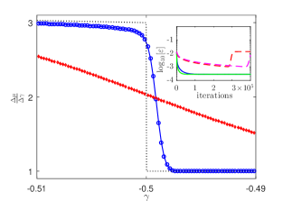
Figure 1: (Color online) Accuracy of the resolution of the discontinuity in the derivative of $\mu$ with the two different numerical methods. The main figure shows the discontinuity at $\gamma=-0.5$. DFPM is shown as a solid line with circles (blue) and 4A00 with diamonds (red). The (black) dotted line is based on the exact solutions of Appendix A. The inset plot shows the instability in $\varepsilon$ of the 4A00-method (dashed) with $\Delta\tau=0.0002$ (red) and $\Delta\tau=0.00015$ (magenta) for $\gamma=-0.501$, while the DFPM (solid) reach a constant $\varepsilon$ both for $\eta=2.2$ (blue) and $\eta=1$ (green).

Both methods converge slower close to the discontinuity and give less accurate solutions as well as chemical potentials. However, the DFPM produces a qualitatively correct step (see Fig. 1), while the 4A00 method performs less well here. In fact it is even worse than Fig. 1 shows. If we let the numerical solvers continue until they stabilize we find that 4A00 diverges; see the inset of Fig. 1 for two examples. We have in fact been unable to find any value of $\Delta\tau$ for which 4A00 stabilizes to a value close to the exact solutions for the range of $\gamma$ values investigated. The DFPM may also fail if the time step is too large but it is always possible to find some $\Delta\tau$ such that convergence is assured.

Changing the damping in the DFPM does affect the speed of convergence somewhat but does not affect the end result as long as the solver is allowed to stabilize. The inset of Fig. 1 also shows the convergence of DFPM for two different values of the damping parameter: $\eta=1.0,\ 2.2$.

III Constraints on the solutions

Ground-state solutions to the NLSE with a nonzero angular momentum are called yrast states. These solutions can be considered as stationary when viewed from a co-rotating frame. If we introduce a new angle coordinate $\theta=\Theta-\Omega\tau$ to the time-dependent NLSE corresponding to (4)

$$i\frac{\partial\Psi}{\partial\tau}=-\frac{\partial^{2}\Psi}{\partial\Theta^{2}}+2\pi\gamma\left|\Psi\right|^{2}\Psi,$$ (12)

and use the ansatz $\Psi\left(\theta\right)=\Psi\left(\Theta\right)\exp\left(i\Omega\tau\right)$, we obtain from (12) the following equation in the coordinate $\theta$:

$$-\frac{\partial^{2}\Psi}{\partial\theta^{2}}+i\Omega\frac{\partial\Psi}{\partial\theta}+2\pi\gamma\left|\Psi\right|^{2}\Psi=\mu\Psi.$$ (13)

The corresponding angular momentum is given by the functional,

$$\ell=-i\int_{-\pi}^{\pi}\overline{\Psi}\frac{\partial\Psi}{\partial\theta}\mathrm{d}\theta.$$ (14)

Alternatively to the time-dependent NLSE (12) we can introduce two Lagrange multipliers corresponding to the chemical potential and the angular velocity, respectively, $\lambda^{1}:=\mu$ for the normalization constraint (6), and $\lambda^{2}:=\Omega$ for the additional constraint,

$$g_{2}[\Psi]:=-i\int_{-\pi}^{\pi}\overline{\Psi}\frac{\partial\Psi}{\partial\theta}\mathrm{d}\theta-\ell_{0}=0,$$ (15)

for some fixed value $\ell_{0}$ of the angular momentum. Minimizing the following functional,

$$E_{\lambda}\left[\Psi\right]=E[\Psi]-\lambda^{A}g_{A}[\Psi],$$ (16)

is then equivalent to finding the ground-state solution to (12), since (13) is the corresponding Euler equation to (16). Einstein’s summation convention applies to all index pairs that appears both as superscript and subscript.

The DFPM can be used for problems with constraints straightforwardly. As before, instead of solving (13) directly, we consider the time-dependent unphysical problem,

$$\frac{\partial^{2}\Psi}{\partial\tau^{2}}+\eta\frac{\partial\Psi}{\partial\tau}=F[\Psi]+\lambda^{A}G_{A}[\Psi],$$ (17)

where $F[\Psi]:=-\delta E[\Psi]/\delta\overline{\Psi}$, $G_{A}[\Psi]:=\delta g_{A}[\Psi]/\delta\overline{\Psi}$ are defined by functional derivation of the energy and constraint functionals, respectively.

We have chosen to solve (17) by a modified version of the second-order symplectic method RATTLE Andersen (1983), originally considered to handle separable Hamiltonians with constraints. As a first step we once again rewrite (17) as a first-order system similar to (9)

$$\dot{q}= p,$$ (18)

$$\dot{p}= F[q]+\lambda^{A}G_{A}[q]-\eta p,\quad A=1,2.$$

To solve this system numerically we discretize in space as before and use the RATTLE method for the time evolution, with the modification that the nonsymplectic part of (18) modifies the update of the momentum according to

$$p^{i}_{n+1/2}= p^{i}_{n}+\dfrac{\Delta\tau}{2}\left(F[q^{i}_{n}]+\lambda_{n}^{A}G_{A}[q^{i}_{n}]-\eta p^{i}_{n}\right),$$ (19)

$$q^{i}_{n+1}= q^{i}_{n}+\Delta\tau p^{i}_{n+1/2},$$

$$0= g_{A}[q^{i}_{n+1}],\quad A=1,2,$$

$$p^{i}_{n+1}= p^{i}_{n+1/2}+\dfrac{\Delta\tau}{2}\left(F[q^{i}_{n+1}]+\tilde{\lambda}_{n}^{A}G_{A}[q^{i}_{n+1}]-\eta p^{i}_{n+1/2}\right),$$

$$0= \int_{-\pi}^{\pi}\overline{G_{A}[q_{n+1}]}p^{i}_{n+1}\mathrm{d}\theta,\quad A=1,2.$$

The last equation above is a projection step to ensure that the update of $p^{i}_{n}$ is tangent to the constraint surface. The integral is performed with the trapezoidal approximation. The constraints $g_{A}[q^{i}_{n+1}]$ are quadratic algebraic equations in the Lagrange multipliers $\lambda_{n}^{A}$, and are solved with Newton’s method for each time step $n$. The linear projection equation is solved for a second set of Lagrange multipliers $\tilde{\lambda}_{n}^{A}$ (see Chapter VII of Hairer et al. (2006)) that coincide with $\lambda_{n}^{A}$ in the limit of the stationary solution.

Our goal here is to obtain $E$ from (5) as a function of the angular momentum $\ell$ that is given by the functional (14). Hence, given a fixed value for the angular momentum, $\ell_{0}$, we solve the constraints and Eq. (13) for $\mu,\>\Omega$ and $\Psi$. Having found this $\Psi$, the energy $E$ is calculated from (5) and we plot the so-called yrast curve $E\left(\ell\right)$ (see Fig. 2).

We used a grid of $N=400$ points, a damping parameter $\eta=2.74$, and time step $\Delta\tau=0.015$. Initial data were chosen for each run as $q^{j}_{0}=\left(a+\sqrt{\ell_{0}/k}\exp(ikx^{j})\right)/(\sqrt{2\pi})$, $p^{j}_{0}=0$, where $k$ is the nearest integer with absolute value larger than or equal to $|\ell_{0}|$ and $a$ is chosen such that the normalization is equal to 1. These initial data satisfied both constraints and produced good results for all $|\ell_{0}|<1$ but not for larger values. For these we insted used a $k$ that had an absolute value that was the next larger integer.

In Appendix B we outline how to implicitly represent the yrast curve in terms of elliptic integrals and Jacobi elliptic functions, that we have used to benchmark the numerical results. At integer values of the angular momentum, the ground-state solutions to the NLSE are the plane-wave states,

$$\varphi_{k}(\theta)=\exp(ik\theta)/\sqrt{2\pi}.$$ (20)

As a check of the numerical results we also plot the energy of these states in Fig. 2.

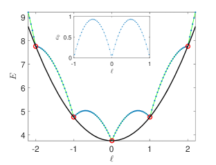
Figure 2: (Color online) Yrast curve for the single-component NLSE with $\gamma=7.5$. The figure compares the numerical results with the values derived from the analytic solutions given in Appendix B and verifies Bloch’s formula (21) numerically. The (blue) dots show numerical results from solving Eqs. (13) and (14) with the DFPM (19). The thin (green) solid line shows the yrast curve obtained from the analytic results given in Appendix B. The energy of the plane-wave states (20) are indicated as (red) circles. The quadratic $\ell$ dependence for the energy is shown as a thick solid (black) line and the numerical realization of the periodic function $e_{0}(\ell)$ is obtained by subtracting the black curve from the main numerical data and is plotted in the inset figure with (blue) dots connected by a dotted line.

According to Bloch’s theorem Bloch (1973), the energy can be split into a constant part, a part with quadratic dependence on $\ell$, and a periodic and symmetric part,

$$E(\ell)=\gamma/2+\ell^{2}+e_{0}(\ell).$$ (21)

Both the periodicity and symmetry of $e_{0}(\ell)$ is verified numerically as seen in the inset of Fig. 2.

The solution to the DFPM preserves the constraints numerically to a given set tolerance at each time step and converges to an approximation of order $h^{2}$ to the solution of the continuous NLSE. An alternative method often used for solving the constrained NLSE is the so-called penalty method Komineas et al. (2005) where the functional,

$$E_{w}\left[\Psi\right]=E\left[\Psi\right]+\frac{w}{2}\left(g_{2}[\Psi]\right)^{2},$$ (22)

is minimized for a constant weight $w$. The drawback with the penalty method is that the minimum of this functional is not the minimum of $E\left[\Psi\right]$ and that the momentum of the solution will not be $\ell_{0}$, but some value close to $\ell_{0}$. The weight $w$ in (22) has to be chosen such as to balance the error in the original energy functional with the error in the angular momentum constraint, since they can not attain minimal value at the same time. The DFPM presented has none of these drawbacks.

IV Constraints for Two-component systems

Experiments on persistent currents in toroidal two-component Bose gases Beattie et al. (2013) have motivated theoretical investigation of the coupled multi component NLSE on a ring geometry Wu and Zaremba (2013); Wu et al. (2015). The multi component NLSE can be solved numerically with the DFPM with only minor modification from the constrained single-component case if we consider the two species as components of a vector-valued mean-field wave function. The main difference here is that we now have three constraints instead of two, and that the nonlinearity parameter becomes a matrix-valued coupling between the different components.

Let $\Psi_{s},\>s=1,2$ denote the mean-field wave functions of the two components. Each component satisfies a normalization constraint $\int\overline{\Psi_{s}}\Psi_{s}\mathrm{d}\theta=x_{s}$, where the total normalization sums up to unity, $x_{1}+x_{2}=1$. The yrast states are obtained using the further constraint that the total angular momentum is constant, $-i\int\left(\overline{\Psi}_{1}\frac{\partial\Psi_{1}}{\partial\theta}+\overline{\Psi}_{2}\frac{\partial\Psi_{2}}{\partial\theta}\right)\mathrm{d}\theta=\ell_{0}$. All three constraints can be written on the general form,

$$\int_{-\pi}^{\pi}\boldsymbol{\Psi}^{\dagger}\boldsymbol{K}_{A}\boldsymbol{\Psi}\mathrm{d}\theta=c_{A},$$ (23)

for $(c_{A})=(x_{1},\>x_{2},\>\ell_{0})$, and three different matrices of operators,

$$\boldsymbol{K}_{1}=\begin{bmatrix}{\rm I}&0\\ 0&0\end{bmatrix},\>\boldsymbol{K}_{2}=\begin{bmatrix}0&0\\ 0&{\rm I}\end{bmatrix},\>\boldsymbol{K}_{3}=-i\begin{bmatrix}\frac{\partial}{\partial\theta}&0\\ 0&\frac{\partial}{\partial\theta}\end{bmatrix},$$ (24)

where I denotes the identity map, acting on $\boldsymbol{\Psi}$, with the conjugate transpose $\boldsymbol{\Psi}^{\dagger}=\begin{bmatrix}\overline{\Psi}_{1}&\overline{\Psi}_{2}\end{bmatrix}$. The problem is then to find the minimum of the two-component energy-functional

$$E[\boldsymbol{\Psi}]=\int_{-\pi}^{\pi}\boldsymbol{\Psi}^{\dagger}\left(-\frac{\partial^{2}}{\partial\theta^{2}}+\pi\boldsymbol{\Gamma}_{\Psi}\right)\boldsymbol{\Psi}\mathrm{d}\theta,$$ (25)

subject to the constraints, which are added to the energy-functional together with the triplet of Lagrange multipliers $\lambda^{A}=(\mu_{\text{1}},\mu_{2},\Omega)$, resulting in the constrained energy functional,

$$E_{\lambda}[\boldsymbol{\Psi}] =E[\boldsymbol{\Psi}]+\lambda^{A}\left(c_{A}-\int_{-\pi}^{\pi}\boldsymbol{\Psi}^{\dagger}\boldsymbol{K}_{A}\boldsymbol{\Psi}\mathrm{d}\theta\right),$$ (26)

where

$$\boldsymbol{\Gamma}_{\boldsymbol{\Psi}}=\begin{bmatrix}\gamma_{11}|\Psi_{1}|^{2}&\gamma_{12}\Psi_{1}\overline{\Psi}_{2}\\ \gamma_{21}\Psi_{2}\overline{\Psi}_{1}&\gamma_{22}|\Psi_{2}|^{2}\end{bmatrix}.$$ (27)

Variation with respect to $\boldsymbol{\Psi}^{\dagger}$ gives the corresponding coupled NLSEs,

$$-\frac{\partial^{2}\boldsymbol{\Psi}}{\partial\theta^{2}}+2\pi\boldsymbol{\Gamma}_{\boldsymbol{\Psi}}\boldsymbol{\Psi}-\lambda^{A}\boldsymbol{K}_{A}\boldsymbol{\Psi}=0.$$ (28)

Using a discretization of $N=400$ points, i.e., a state vector $q^{i}_{n}$ with $2N$ points, representing both components, we can use the DFPM formulation (19) to solve Eq. (28).

As an example, we use the parameter values $x_{1}=0.8,\>x_{2}=0.2,\>\gamma_{11}=\gamma_{22}=1250/\pi^{2},\>\gamma_{12}=\gamma_{21}=750/\pi^{2}$, and solve Eq. (28) for 460 values of $\ell$ between -2.2 and 2.2. The resulting yrast curve is shown in Fig. 3. The equations were solved for $\ell$ in sequence, where initial data for the next run was given by the solution from the last. The damping parameter was initially set to 1. Sometimes the solver gave solutions with too high a value for the energy and then the damping parameter was halved and the solver restarted with the lower value for the damping until a solution with an energy close to the last point on the curve (presumably being the yrast state) was found.

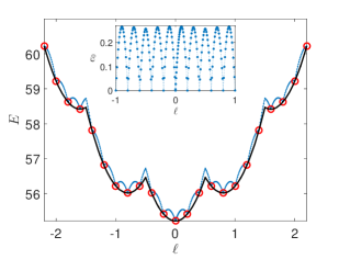
Figure 3: (Color online) Yrast curve for the two-component NLSE. The figure is the two-component analog to Fig. 2. The main figure shows both numerical results obtained using the algorithm (19), indicated by (blue) dots connected by a thin solid line to guide the eye, and analytic results from the plane-wave solutions of Eq. (29), indicated as (red) circles. In addition, the nonperiodic component of the function (30), $E_{\mathrm{int}}+P_{0}(\ell)$ is plotted as a thick (black) solid line. The inset figure shows the numerical data for the periodic part of the yrast curve, $e_{0}$, which is obtained by subtracting the black curve from the numerical data in the main figure.

As a check of the results we also plot the energies of the analytic two-component plane-wave states that should lie on the yrast curve as local minima of the energy for the parameters chosen here Wu et al. (2015). The plane-wave states are given by $\Psi_{s}(\theta)=\sqrt{x_{s}/2\pi}\exp(ik_{s}\theta)$, and the total energy and angular momentum of these states are according to (23) and (25)

$$E =x_{1}k_{1}^{2}+x_{2}k_{2}^{2}+E_{\mathrm{int}},$$ (29)

$$\ell =x_{1}k_{1}+x_{2}k_{2},$$

with $E_{\mathrm{int}}=\left(\gamma_{11}x_{1}^{2}+\gamma_{22}x_{2}^{2}+\gamma_{12}x_{1}x_{2}+\gamma_{21}x_{1}x_{2}\right)/2$. We have plotted $E(\ell)$ of (29) as circles in the yrast curve for a subset of integer wave numbers $k_{s}$ between -3 and 3. The numerical results of the DFPM coincide with the analytic solutions of (29) at the points where the plane-wave solutions are applicable (see Fig. 3).

As illustrated in Fig. 2, the energy of the single-component NLSE yrast state can be split into one part with quadratic dependence of the angular momentum and one part that is periodic Bloch (1973). One can see from Fig. 3 that the two-component yrast curve has two different quadratic energy scales, corresponding to the majority- ($x_{1}=0.8$) component and the minority- ($x_{2}=0.2$) component, respectively. There is a major quadratic dependence $P_{1}(\ell)=\ell^{2}/x_{1}$, and superimposed on this function there are smaller parabolas $P_{2}^{n}(\ell)=(\ell-nx_{1})^{2}/x_{2},\>n\in\mathbb{Z}$. The yrast curve is determined by the lowest energy value of these quadratic functions plus a part, $e_{0}(\ell)$, that is periodic and symmetric,

$$E(\ell)=E_{\mathrm{int}}+P_{0}(\ell)+e_{0}(\ell),$$ (30)

where

$$P_{0}(\ell) = \underset{n\in\mathbb{Z}}{\min}\left\{P_{1}(nx_{1})+P_{2}^{n}(\ell)\right\}$$

$$= \left[\ell\right]^{2}x_{1}+(\ell-\left[\ell\right]x_{1})^{2}/x_{2}.$$

Here $\left[\ \right]$ denotes the nearest integer function. Subtracting the function $E_{\mathrm{int}}+P_{0}(\ell)$ from the numerical data of the energy gives the periodic function $e_{0}(\ell)$ (see inset of Fig. 3).

V Conclusions

We have validated the dynamical functional particle method (DFPM) numerically for retrieving stationary solutions of the nonlinear Schrödinger equation (1). With an attractive (negative) interaction parameter, the method managed well in resolving a quantum phase transition, which seems difficult with other numerical methods, and could reproduce analytic results in the limit of an increasing numbers of grid points. For a repulsive (positive) interaction parameter we added a constraint on the angular momentum, which allows for nontrivial solutions, and reproduced the so-called yrast curve numerically up to machine precision. Finally, we added a second component together with a constraint on the total angular momentum, for which we calculated a corresponding yrast curve.

The method we have developed can be generalized in dimensionality, in the number of components, and in the number of and type of constraints. Hence, the method may be used in a wide range of future applications.

VI Acknowledgments

The authors acknowledge support from Örebro University, School of Science and Technology, and partly through RR 2015/2016. We thank G. M. Kavoulakis for useful discussions.

Appendices: Reference solutions for the benchmarking of the numerical method

We here give the analytic formulas used as reference solutions for the numerical simulations presented in Secs. II and III of the article.

Appendix A The NLSE on a ring with attractive interaction

The NLSE presented in Eq. (4) gives rise to a quantum phase transition for a critical negative value of the parameter $\gamma$ in the nonlinear term. For $\gamma\geq-1/2$ the density is uniform, while for $\gamma<-1/2$ a peak develops in the ground-state density Kanamoto et al. (2003); Kavoulakis (2003). For $\gamma<-1/2$ the wave function can be expressed as Carr et al. (2000a)

$$\Psi=\sqrt{\frac{\textrm{K}\left(m\right)}{2\pi\textrm{E}\left(m\right)}}\textrm{dn}\left(\frac{\textrm{K}\left(m\right)}{\pi}\Theta,m\right),$$ (32)

where K and E are the complete elliptic integrals of the first and second kind, and dn is a Jacobi elliptic function Abramowitz and Stegun (1964). In order to chose the dimensionless parameter $0\leq m<1$ for a given value of $\gamma<-1/2$, the following equation is solved Kanamoto et al. (2003)

$$\textrm{K}\left(m\right)\textrm{E}\left(m\right)=-\frac{\pi^{2}\gamma}{2}.$$ (33)

As we can see from a power series expansion in $m$ of the elliptic integrals, $\textrm{K}\left(m\right)\sim\pi/2\left(1+m/4+9m^{2}/64+...\right)$ and $\textrm{E}\left(m\right)\sim\pi/2\left(1-m/4-3m^{2}/64+...\right)$, the critical coupling $\gamma\rightarrow-1/2^{-}$ corresponds to $m\rightarrow 0^{+}$. We can then relate $\gamma$ and $m$ in this limit from (33) according to

$$\frac{dm}{d\gamma}=\frac{-4}{\sqrt{-\gamma-1/2}}.$$ (34)

The derivative of the chemical potential, i.e., the lowest eigenvalue of Eq. (4) which according to Kanamoto et al. (2003) is

$$\mu=\left\{\begin{array}[]{ll}\gamma,&\gamma\geq-1/2\\ -\frac{\textrm{K}^{2}\left(m\right)\left(2-m\right)}{\pi^{2}},&\gamma<-1/2\end{array}\right.,$$ (35)

with respect to the parameter $\gamma$, is discontinuous at the critical value $\gamma=-1/2$ and can there be expressed with the help of (34) according to

$$\frac{\partial\mu}{\partial\gamma}=\frac{dm}{d\gamma}\frac{d\mu}{dm}\rightarrow\left\{\begin{array}[]{ll}1,&\gamma\rightarrow-1/2^{+}\\ 3,&\gamma\rightarrow-1/2^{-}\end{array}\right..$$ (36)

This explains the step seen in Fig. 1, which is a critical test for the accuracy of a numerical method.

Appendix B The NLSE on a ring with repulsive interaction and a constrained angular momentum

The density of the ground state is always uniform for a positive parameter $\gamma$ in the nonlinear term of Eq. (4). However, exciting the ring system to a constrained value of the (normalized) angular momentum $0<\ell<1$ form gray solitary waves with a nonuniform density in the rotating frame Carr et al. (2000b); Smyrnakis et al. (2010). It was recently pointed out that those solitary waves are indeed the lowest rotational excitations discussed in the concept of the so called yrast curve, i.e., the states with the lowest energy given an angular momentum $0<\ell<1$ Kanamoto et al. (2010); Jackson et al. (2011). In order to benchmark the numerical simulations for the constrained NLSE presented in Sec. III, we have compared with an alternative representation of the yrast curve which we have based on the work presented in Smyrnakis et al. (2010); Jackson et al. (2011). We use again a dimensionless parameter $0\leq m<1$ but now to parametrize the angular momentum $\ell\left(m\right)$ and the lowest energy $E\left(m\right)$ given the constraint, in order to plot the yrast curve with $E$ versus $\ell$, see Fig. 2. With an ansatz $\Psi=\sqrt{n}\exp\left(i\phi\right)$ for the complex wave function with density $n\left(m\right)=\left|\Psi\right|^{2}$ (normalized to unity) and a phase $\phi\left(m\right)$, the normalized angular momentum (14) can be written as

$$\ell\left(m\right)=\int_{-\pi}^{\pi}n\frac{\partial\phi}{\partial\theta}\mathrm{d}\theta.$$ (37)

Above we have used that $n\left(\theta\right)$ is an even function, such that the integral of its derivative disappears. For the normalized energy (5) we have

$$E\left(m\right)=\int_{-\pi}^{\pi}\left[\left(\frac{\partial\sqrt{n}}{\partial\theta}\right)^{2}+n\left(\frac{\partial\phi}{\partial\theta}\right)^{2}+\pi\gamma n^{2}\right]\mathrm{d}\theta,$$ (38)

where we have used that $1/\left(2\sqrt{n}\right)\partial n/\partial\theta=\partial\sqrt{n}/\partial\theta$. Below we give our parametrizations of the density,

$$n\left(m\right)=\frac{1}{2\pi}-\frac{\textrm{K}\left[\textrm{K}-\textrm{E}-m\textrm{K}\textrm{sn}^{2}\left(\frac{\textrm{K}}{\pi}\theta,m\right)\right]}{\pi^{3}\gamma},$$ (39)

and the phase

$$\frac{\partial\phi}{\partial\theta}\left(m\right)=\frac{1}{8\pi^{5}\gamma}\sqrt{abc}\left[\int_{-\pi}^{\pi}\frac{1}{n\left(m\right)}\mathrm{d}\theta-\frac{2\pi}{n\left(m\right)}\right],$$ (40)

$$\begin{array}[]{l}a=4m\textrm{K}^{2}+4\textrm{E}\textrm{K}-4\textrm{K}^{2}+2\pi^{2}\gamma,\\ b=2\textrm{E}\textrm{K}-2\textrm{K}^{2}+\pi^{2}\gamma,\\ c=2\textrm{E}\textrm{K}+\pi^{2}\gamma,\end{array}$$

which are needed above in Eqs. (37) and (38) in order to produce the yrast curve for a given $\gamma-$parameter. Again K and E are the complete elliptic integrals of the first and second kind, and sn is a Jacobi elliptic function with derivative $\partial\textrm{sn}\left(\theta,m\right)/\partial\theta=\textrm{cn}\left(\theta,m\right)\textrm{dn}\left(\theta,m\right)$ Abramowitz and Stegun (1964), such that $\partial\sqrt{n}/\partial\theta\left(m\right)=\textrm{K}^{3}m\>\textrm{sn}\>\textrm{cn}\>\textrm{dn}/\left(\pi^{4}\gamma\sqrt{n\left(m\right)}\right)$. Note that here the dimensionless parameter $0\leq m<1$ can be chosen arbitrarily in order to cover the range $0\leq\ell<1/2$, while in practice one needs a non-equidistant domain of $m$-values to produce an yrast curve that is equidistant in the $\ell$ variable. The continuation of the yrast curve to $1/2<\ell\leq 1$ can then be obtained directly with so-called Bloch mapping Bloch (1973). In a similar way we can get even the full range $-\infty<\ell<\infty$ (see Fig. 2).

References

- Fibich (2015) G. Fibich, The Nonlinear Schrödinger Equation (Springer, New York, 2015).
- Abdullaev et al. (2011) F. K. Abdullaev, V. V. Konotop, M. Ögren, and M. P. Sørensen, Opt. Lett. 36, 4566 (2011).
- Ögren et al. (2012) M. Ögren, M. Sørensen, and N. Pedersen, Physica C 479, 157 (2012).
- Nielsen and Olesen (1973) H. Nielsen and P. Olesen, Nuclear Physics B 61, 45 (1973).
- Chavanis (2011) P.-H. Chavanis, Phys. Rev. D 84, 043531 (2011).
- Andersen et al. (1995) M. H. Andersen, J. R. Ensher, M. R. Matthews, C. E. Wieman, and E. A. Cornell, Science 269, 198 (1995).
- Bradley et al. (1995) C. C. Bradley, C. A. Sackett, J. J. Tollett, and R. G. Hulet, Phys. Rev. Lett. 75, 1687 (1995).
- Davis et al. (1995) K. B. Davis, M. O. Mewes, M. R. Andrews, N. J. van Druten, D. S. Durfee, D. M. Kurn, and W. Ketterle, Phys. Rev. Lett. 75, 3969 (1995).
- Ensher et al. (1996) J. R. Ensher, D. S. Jin, M. R. Matthews, C. E. Wieman, and E. A. Cornell, Phys. Rev. Lett. 77, 4984 (1996).
- Dalfovo et al. (1996) F. Dalfovo, L. P. Pitaevskii, and S. Stringari, J. Res. Natl. Inst. Stand. Technol. 101, 537 (1996).
- Bao et al. (2006) W. Bao, I. L. Chern, and F. Y. Lim, J. of Comp. Phys. 219, 836 (2006).
- Mallory and Van Gorder (2015) K. Mallory and R. A. Van Gorder, Phys. Rev. E 92, 013201 (2015).
- Mocz and Succi (2015) P. Mocz and S. Succi, Phys. Rev. E 91, 053304 (2015).
- Taha and Ablowitz (1984) T. R. Taha and M. J. Ablowitz, J. of Comp. Phys. 55, 203 (1984).
- Cerimele et al. (2000a) M. M. Cerimele, F. Pistella, and S. Succi, Comput. Phys. Commun. 129, 83 (2000a).
- Cerimele et al. (2000b) M. M. Cerimele, M. L. Chiofalo, F. Pistella, S. Succi, and M. P. Tosi, Phys. Rev. E 62, 1382 (2000b).
- Palpacelli and Succi (2008) S. Palpacelli and S. Succi, Phys. Rev. E 77, 066708 (2008).
- Mendoza et al. (2014) M. Mendoza, S. Succi, and H. J. Herrmann, Phys. Rev. Lett. 113, 096402 (2014).
- Ruprecht et al. (1995) P. A. Ruprecht, M. J. Holland, K. Burnett, and M. Edwards, Phys. Rev. A 51, 4704 (1995).
- Chin and Krotscheck (2005) S. A. Chin and E. Krotscheck, Phys. Rev. E 72, 036705 (2005).
- Mueller and Ho (2002) E. J. Mueller and T.-L. Ho, Phys. Rev. Lett. 88, 180403 (2002).
- Abdullaev et al. (2013) F. K. Abdullaev, M. Ögren, and M. P. Sørensen, Phys. Rev. A 87, 023616 (2013).
- Edvardsson et al. (2012) S. Edvardsson, M. Gulliksson, and J. Persson, Journal of Applied Mechanics 79, 021012 (2012).
- Gupta et al. (2005) S. Gupta, K. W. Murch, K. L. Moore, T. P. Purdy, and D. M. Stamper-Kurn, Phys. Rev. Lett. 95, 143201 (2005).
- Hairer et al. (2006) E. Hairer, G. Wanner, and C. Lubich, Geometric Numerical Integration (Springer, Berlin/Heidelberg, 2006).
- Andersen (1983) H. C. Andersen, J. of Comp. Phys. 52, 24 (1983).
- Bloch (1973) F. Bloch, Phys. Rev. A 7, 2187 (1973).
- Komineas et al. (2005) S. Komineas, N. R. Cooper, and N. Papanicolaou, Phys. Rev. A 72, 053624 (2005).
- Beattie et al. (2013) S. Beattie, S. Moulder, R. J. Fletcher, and Z. Hadzibabic, Phys. Rev. Lett. 110, 025301 (2013).
- Wu and Zaremba (2013) Z. Wu and E. Zaremba, Phys. Rev. A 88, 063640 (2013).
- Wu et al. (2015) Z. Wu, E. Zaremba, J. Smyrnakis, M. Magiropoulos, N. K. Efremidis, and G. M. Kavoulakis, Phys. Rev. A 92, 033630 (2015).
- Kanamoto et al. (2003) R. Kanamoto, H. Saito, and M. Ueda, Phys. Rev. A 67, 013608 (2003).
- Kavoulakis (2003) G. M. Kavoulakis, Phys. Rev. A 67, 011601 (2003).
- Carr et al. (2000a) L. D. Carr, C. W. Clark, and W. P. Reinhardt, Phys. Rev. A 62, 063611 (2000a).
- Abramowitz and Stegun (1964) M. Abramowitz and I. A. Stegun, Handbook of Mathematical Functions: With Formulas, Graphs, and Mathematical Tables, 55 (Courier Corporation, North Chelmsford, 1964).
- Carr et al. (2000b) L. D. Carr, C. W. Clark, and W. P. Reinhardt, Phys. Rev. A 62, 063610 (2000b).
- Smyrnakis et al. (2010) J. Smyrnakis, M. Magiropoulos, G. M. Kavoulakis, and A. D. Jackson, Phys. Rev. A 82, 023604 (2010).
- Kanamoto et al. (2010) R. Kanamoto, L. D. Carr, and M. Ueda, Phys. Rev. A 81, 023625 (2010).
- Jackson et al. (2011) A. D. Jackson, J. Smyrnakis, M. Magiropoulos, and G. M. Kavoulakis, Europhys. Lett. 95, 30002 (2011).