center

On fields inspired with the polar $HSV-RGB$ theory of Colour

Ján Haluška

1 Introduction

1.1 Traditional Colour theories

There are more different sources of the theory of Colour which approach to the subject from different sides and are complementary in this sense.

Computer graphics

The HSV (Hue-Saturation-Value) theory is the most common representation of points in an RGB (Red-Green-Blue) color technical model. Computer graphics pioneers developed the HSV model in the 1970s for computer graphics applications (A. R. Smith in 1978, also in the same issue, A. Joblove and H. Greenberg). A HSV theory is used today in color pickers, in image editing software, and less commonly in image analysis and computer vision. A rather extensive explanation of the present State of Art in industry we can find in [11].

Biophysics

Th. Young and H. Helmholtz proposed a trichromatic theory. Their theory states that the human retina contains dispersed photo-sensitive clusters, where each of these clusters consists of three types of sensitive cones which peaks in short (420–440 nm), middle (530–540 nm), and long (560–580 nm) wavelengths. Weighting a total light power spectrum by the individual spectral sensitivities of the three types of cone cells gives three effective stimulus values; these three values make up a tristimulus specification of the objective color of the light spectrum. In Fig. 1, there are schematic behaviours of these sensitive clusters of cells.

Fine arts

For the revelatory theories of Colour written by authors who are not mathematicians (artistic photographers, visual artists), c.f. [1, 6, 7].

1.2 Terminology

For terminology, basic and also advanced concepts about Colour, we refer to [12], Chapter 11 (Vol. III, Vision and vision optics; Chap. 11, Color vision mechanism).

1.3 Comments to modelling of Colour

A reflected electro-magnetic vibration energy is filtered with the (human) tristimulus apparatus in the eye retina into three functions (also called the $RGB$ stimulus curves). Here is an information loss, because we see in the wavelength interval approximately 350 nm – 750 nm although there is some power output theoretically within the whole $[0,+\infty)$. Vibrations within other vibration intervals are partially perceived by other senses (hearing, touch). Also variuos animals have various intervals within they can see. The vision process continues in the brain where the obtained three stimuli curves are aggregated back. The result is a registry of Colour of the object. In our theory, this aggregation is a linear combination of three basic colours (poles) with the coefficients which are complex functions defined on the interval $[0,+\infty)$ (= all possible frequencies). In Fig. 1, we see that realistic stimulus curves may have parts which are particularly in the negative (under the $x$-axis), i.e., the accession to the resulting Colour may happen also such that the parts of curves "absorbs" energy. Some practical aspects about $RGB$ in computer graphics we can find in [10].

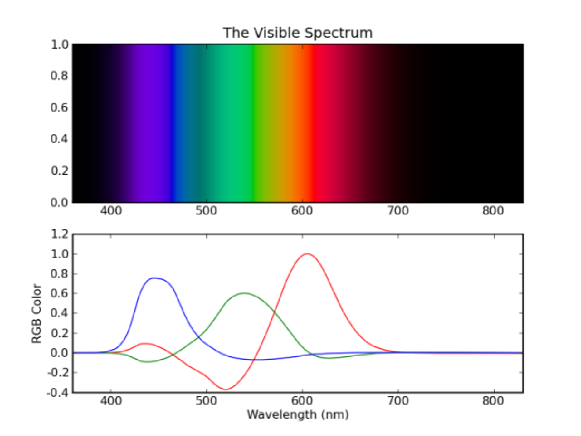
Figure 1: A realistically shaped tristimulus reaction on a Colour

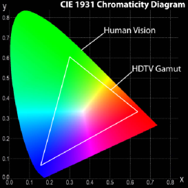
Figure 2: A horse-shoe planar cut of the visible colour space; Black = non visible

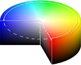
Figure 3: A Colour wheel with colours of the equal energy (the upper surface)

Outside a certain area of the domain, the colour aggregated from $R,B,G$ curves is not very exact because of distorted perceptions by human senses, see Fig. 2. We use an imagination of the Colour Hues in the Colour wheel. The reason is that there are colour hues which are not in the linear rainbow palette (e.g., Pink). We suppose that angles of the basic $RGB$ colours in the colour wheel correspond to the angles $0\equiv 2\pi$, $2\pi/3$, $4\pi/3$, respectively, which is approximately true in reality. An incoming white sun light is Colours is decomposed into a sum of three $RGB$ curves. So it is also in our model. But abstracting from the natural perception, the number three for basic colours is not substantial. Our polar theory works for arbitrary natural $K\geq 3$. For a review, in the realm of animals, there are mono-chromatic Arctic mammals; most of mammals have sensibility only for two colours, they are dichromats; birds and insects are mostly tetrachromats. Concerning primates, the human vision is trichromatic. The record keeps the Mantis shrimp’s vision with $K=12$, cf. [13]. There are also artificial colour schemes coming and used in the industry for some good reasons. E.g., we know the CMYK (cyan, magenta yellow, black), RGYB (red, green, yellow, blue) systems, and others.

1.4 The point and interval characteristics of light

Hue is a point characteristic (it is determined in a point), the saturation and brightness are "interval" characteristics, i.e., they are determined for an interval, not at a point (similarly as the notions concavity-convexity has no sense at a points).

Hue

of Colour is the wavelength within the visible-light spectrum at which the energy output from a source is greatest. This is shown as the peak of the sum of the three intensity curves in the accompanying graphs of intensity versus wavelength. In the illustrative examples in the pictures Fig.4, Fig.5, Fig.6, all $3\times 3$ = nine colors there have the same Hue with a wavelength 500 nm, in the yellow-green portion of the spectrum.

Saturation

is an expression for the relative bandwidth of the visible output from a light source. In the diagram Fig.4, the notion of saturation is represented relatively, by the steepness of the slopes of the curves. Here, the blue curve represents a color having the greatest saturation. As saturation increases, the color with the same Hue appears more "pure." As saturation decreases, colors appear more "washed-out."

Brightness

is a relative expression of the intensity of the energy output of a visible light source. It can be expressed as a total energy value (different for each of the curves in the diagram Fig. 5), or as the amplitude at the wavelength where the intensity is greatest. Energy is imagined as the area under the curve. In the picture the blue curve has the lowest brightness. As we can see, Saturation and Brightness are generally non-comparable parameters of Colour, cf. Fig.6. One commonly supposes that all possible colours can be specified according to these three parameters and that Colors can be represented in terms of the $RGB$ components. Thus the whole information in the $RBG$ Colour theory is contained the three tristimulus curves. A concept of triangular coefficients mathematically reflects this idea.

1.5 Semi-field of triangular coefficients

A semi-field $\mathbb{X}$ is a set equipped with an algebraic structure with binary operations of addition $(+)$ and multiplication $(\cdot)$, where $(\mathbb{X},+)$ is a commutative semi-group. $(X,\cdot,1)$ is a multiplicative group with the unit $1$, and multiplication is distributive with respect to addition from both sides. For a review of semi-fields, c.f. [14]. A semi-field $\mathbb{X}$ is called a semi-field with zero if there exists an element $\mathbb{O}\in\mathbb{X}$ such that $\mathbf{x}\cdot\mathbb{O}=\mathbb{O}$ and $\mathbf{x}+\mathbb{O}=\mathbf{x}$ for every $\mathbf{x}\in\mathbb{X}$ and the distributivity of multiplication from both sides is preserved for the extended system.

Example 1.1

Let $\mathbb{R}_{+,0}:=(0,\infty)\cup\{0\}=[0,\infty)$ be a ray with all structures heredited from the real line $\mathbb{R}$. This is one of trivial real semi-field with zero.

Definition 1.2

We say that a set

$$T=\{q+\psi(f)\varepsilon\mid q\geq 0,\psi(f)\in\mathbb{R}^{[0,+\infty)},f\in[0,+\infty)\}$$

is called to be the set of all triangular coefficients, where $\varepsilon$ is the parabolic imaginary unit, $|\varepsilon|=1,\varepsilon^{2}=0$, cf. [5]. If $[a+b(f)\varepsilon]\in T$ and $[A+B(f)\varepsilon]\in T$ are two triangular coefficients, we define the operations of addition, multiplication, and division as following. For every $a,A\geq 0$; $b(f),B(f)\in\mathbb{R}^{[0,+\infty)}$, $f\in[0,+\infty)$,

$$[a+b(f)\varepsilon]+[A+B(f)\varepsilon]:=[a+A]+[b(f)+B(f)]\varepsilon,$$ (1)

$$[a+b(f)\varepsilon]\cdot[A+B(f)\varepsilon]:=aA+[aB(f)+Ab(f)]\varepsilon,$$ (2)

$$A\neq 0\implies\frac{a+b(f)\varepsilon}{A+B(f)\varepsilon}:=\frac{a}{A}+\frac{Ab(f)-aB(f)}{A^{2}}\varepsilon.$$ (3)

For the better reading, triangular coefficients are written in square brackets in the sequel of the paper.

Lemma 1.3

The set $T$ with the operations defined in (1), (2), (3) is a semi-field.

Proof.   Saving the denotation of the previous definition we see that $[a+b(f)\varepsilon]+[A+B(f)\varepsilon]\in T$, $[a+b(f)\varepsilon]\cdot[A+B(f)\varepsilon]\in T$, and for $A\neq 0$, $\frac{a+b(f)\varepsilon}{A+B(f)\varepsilon}\in T$. The assertion is an obvious enlargement of the result for parabolic-complex numbers to functions defined on the non-negative real ray. $\Box\;\;$ In our polar theory of Colour, a role of scalars will play elements of the semi-field $T$.

Corollary 1.4

For every function $B(f),f\in[0,+\infty)$, and by (3),

$$A\neq 0\implies\frac{1}{A+B(f)\varepsilon}=\frac{1}{A}+\frac{-B(f)}{A^{2}}\varepsilon\in T.$$

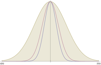
Figure 4: Monotonicity of Saturation; Brightness and Hue are fixed

Figure 5: Monotonicity of Brightness; Saturation and Hue are fixed

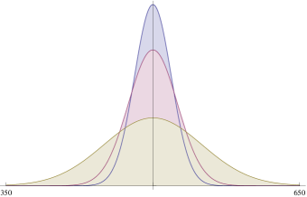
Figure 6: Non-comparable Saturation and Brightness, Hue is fixed

The aim of the paper

To model a Colour space as a three-polar field.

2 Mastering polar Colour spaces

2.1 Poles and the definition of Colour space

The real line is two-polar and we are using the obvious polar operators, i.e., the signs $(+)$ and $(-)$. In this sense, we will also understand three signs (poles) $R,G,B$ in this paper. The poles $R,G,B$ could be understand also as the generalized signs. In fact, poles can be chosen as objects of various mathematical nature. In this paper, we use the following finite set of poles:

$$\mathbb{A}=\left\{R=1+0\imath,G=-\frac{1}{2}+\frac{\sqrt{3}}{2}\imath,B=-\frac{1}{2}-\frac{\sqrt{3}}{2}\imath\right\},$$

a set of three vertices of an equilateral triangle in the elliptic complex plane, where $\imath$ is a usual (elliptic) complex unit, $\imath^{2}=-1$, $|\imath|=1$. Sometimes we will equivalently speak that poles are polar operators.

Remark 2.1

Which properties are asked from poles in general? Various other objects of different nature can also be used as poles. E.g., functions, operators, the set $\mathbb{A}$ when replacing complex unit $\imath$ by the complex units $\varepsilon,\kappa$ of the parabolic ($\varepsilon^{2}=0$) or hyperbolic ($\kappa^{2}=1$) complex units, respectively, etc. In our case, we use the operators $R,G,B\in\mathbb{C}$ which

1. are applicable to "all objects" (similarly as signs plus and minus);

2. fulfil the condition $R+G+B=0$ (presence of the white point of the colour space);

3. $R,G,B$ are different and non-collinear points;

4. a symmetry in some sense of the set $\mathbb{A}$ is desirable.

All these terms will be precised below.

Definition 2.2

Let us denote by

$$\begin{array}[]{rcl}\triangle&:=&\{R[r+\rho(f)\varepsilon]+G[g+\gamma(f)\varepsilon]+B[b+\beta(f)\varepsilon]\\ &&\mid[r+\rho(f)\varepsilon]\in T,[g+\gamma(f)\varepsilon]\in T,[b+\beta(f)\varepsilon]\in T\},\end{array}$$ (4)

where $r,g,b\geq 0$; $\rho(f),\gamma(f),\beta(f)\in\mathbb{R}^{[0,+\infty)},f\in[0,+\infty)$. The set $\triangle$ is called the colour space. An element of the colour space is called to be the colour.

Remark 2.3

(1) Although the functions $\rho(f),\gamma(f),\beta(f)\in\mathbb{R}^{[0,\infty)}$ are arbitrary in our paper, in the praxis they are supposed to have "good" properties, e.g., they are supposed to be unimodal, continuous, etc. (2) Elements of $\triangle$ are (mixed elliptic–parabolic) bicomplex numbers. For (elliptic–elliptic) bicomplex numbers, cf. [8].

2.2 Achromatic part of Colour

Every Colour is a composite of chromatic (pure colours) and achromatic (grey and noises) parts. Both parts of colour can be derived from the decomposition of the tristimulus sum into three individual curves. In this paper, the achromatic part of colour is derived from an element $[a+\alpha(f)]\in T$, where $a\in[0,\infty)$ determines a Hue of Grey. The function $\alpha(f)\in\mathbb{R}^{[0,\infty)}$ represents noise. We incorporate an achromatic part of Colour into our theory dealing with the following subsets (cuts) of the colour space $\triangle$:

Definition 2.4

Let $[a+\alpha(f)\varepsilon]\in T$ and $[r+\rho(f)\varepsilon]\in T$, $[g+\gamma(f)\varepsilon]\in T$, $[b+\beta(f)\varepsilon]\in T$. Denote by

$$\mathfrak{o}_{[a+\alpha(f)\varepsilon]}:=R[a+\alpha(f)\varepsilon]+G[a+\alpha(f)\varepsilon]+B[a+\alpha(f))\varepsilon],$$

$$\mathfrak{O}:=\bigcup_{[a+\alpha(f)\varepsilon]\in T}\mathfrak{o}_{[a+\alpha(f)\varepsilon]}\subset\triangle,$$

and

$$\mathfrak{s}_{a}:=\{\mathbf{x}\in\triangle\mid\mathbf{x}=R[a+\rho(f)\varepsilon]+G[a+\gamma(f)\varepsilon]+B[a+\beta(f)\varepsilon]\},$$

$$\mathfrak{S}:=\bigcup_{a\in[0,\infty)}\mathfrak{s}_{a},$$

where $a\geq 0$ and $\alpha(f),\rho(f),\gamma(f),\beta(f)$ are arbitrary functions in $\mathbb{R}^{[0,\infty)}$.

Lemma 2.5

Let $\mathbf{x}\ \in\triangle$. Let $\lambda\in\mathfrak{O}$. Then

$$\mathbf{x}=\mathbf{x}+\lambda.$$

Proof.   From definition of $\mathfrak{O}$ it follows that the triangular coefficients $[r+\rho(f)\varepsilon]$, $[g+\gamma(f)\varepsilon]$, $[b+\beta(f)\varepsilon]$ in $\mathbf{x}\in\triangle$ are ambiguous since for every arbitrary $[a+\alpha(f)\varepsilon]\in T$, there holds

$$\begin{array}[]{rcl}\mathbf{x}&=\phantom{+}&R[r+\rho(f)\varepsilon]+G[g+\gamma(f)\varepsilon]+B[b+\beta(f)\varepsilon]\\ &=\phantom{+}&R\{[r+\rho(f)\varepsilon]+[a+\alpha(f)\varepsilon]\}\\ &\phantom{=}+&G\{[(g+\gamma(f)\varepsilon]+[a+\alpha(f)\varepsilon]\}\\ &\phantom{=}+&B\{[(b+\beta(f)\varepsilon]+[a+\alpha(f)\varepsilon]\}=\mathbf{x}+\lambda,\lambda\in\mathfrak{O}.\hskip 28.45274pt\Box\end{array}$$

In the view of this lemma we introduce the following notion.

Definition 2.6

Let $X\in\mathbb{A}$. We say that colour $\mathbf{x}\in\triangle$ is $X$-polarized if it can be expressed in the form $\mathbf{x}=X[x+\xi(f)\varepsilon]$, $[x+\xi(f)\varepsilon]\in T$.

Definition 2.7

The congruence given in Lemma 2.5 is known also as the Cancellation law, c.f. [4]). So, (this holds concerning all arithmetic operations in $\triangle$ we will define in the sequel of this paper). So, we operate with the accuracy of congruent triples of triangular coefficients.

Physically Cancellation law means an ambiguity with respect to the achromatic parts of Colour. This is expressed with using of the phrase "with respect to Cancellation law". For the sake of simplicity and without loss of precision, this phrase will be often omitted in the text.

3 Arithmetic operations in $\triangle$

Let us denote for the following sections:

$$\begin{array}[]{rcl}\mathbf{x}&=&\{R[r+\rho(f)\varepsilon]+G[g+\gamma(f)\varepsilon]+B[b+\beta(f)\varepsilon]\}\in\triangle,\\ \mathbf{y}&=&\{R[u+\sigma(f)\varepsilon]+G[v+\chi(f)\varepsilon]+B[t+\xi(f)\varepsilon]\}\in\triangle\end{array}$$

be two colours.

3.1 Addition in $\triangle$ (Mixing of Colours)

We define:

$$\begin{array}[]{rcl}\mathbf{x}\oplus\mathbf{y}&:=&\phantom{+}R\{[r+\rho(f)\varepsilon]+[u+\sigma(f)\varepsilon]\}\\ &&+G\{[g+\gamma(f)\varepsilon]+[v+\chi(f)\varepsilon]\}\\ &&+B\{[b+\beta(f)\varepsilon]+[t+\xi(f)\varepsilon]\},\\ &=&\phantom{+}R[\{r+u\}+\{\rho(f)+\sigma(f)\}\varepsilon]\\ &&+G[\{g+v\}+\{\gamma(f)+\chi(f)\}\varepsilon]\\ &&+B[\{b+t\}+\{\beta(f)+\xi(f)\}\varepsilon].\end{array}$$

Remark 3.1

Remind, that the result of operation of addition is with respect to Cancellation law, i.e., for every $\lambda_{1},\lambda_{2},\lambda_{3}\in\mathfrak{O},$

$$\mathbf{x}\oplus\mathbf{y}=(\mathbf{x}+\lambda_{1})\oplus(\mathbf{y}+\lambda_{2})=(\mathbf{x}\oplus\mathbf{y})+\lambda_{3}.$$

3.2 Subtraction in $\triangle$ (Inverse colours)

We define Subtraction in $\triangle$ as the addition of inverse elements,

$$\mathbf{x}\ominus\mathbf{y}:=\mathbf{x}\oplus(\ominus\mathbf{y}).$$

The inverse elements of the basic colours are defined as follows:

$$\begin{array}[]{ccl}\ominus R[r+\rho(f)\varepsilon]&:=&G[r+\rho(f)\varepsilon]+B[r+\rho(f)\varepsilon],\\ \ominus G[g+\gamma(f)\varepsilon]&:=&R[g+\gamma(f)\varepsilon]+B[g+\gamma(f)\varepsilon],\\ \ominus B[b+\beta(f)\varepsilon]&:=&R[b+\beta(f)\varepsilon]+G[b+\beta(f)\varepsilon].\end{array}$$

So,

$$\begin{array}[]{rcl}\ominus\mathbf{x}&:=&\phantom{+}R\{[g+\gamma(f)\varepsilon]+[b+\beta(f)\varepsilon]\}\\ &&+G\{[r+\rho(f)\varepsilon]+[b+\beta(f)\varepsilon]\}\\ &&+B\{[r+\rho(f)\varepsilon]+[g+\gamma(f)\varepsilon]\}.\end{array}$$

And the subtraction is defined then as following:

$$\begin{array}[]{ccl}\mathbf{x}\ominus\mathbf{y}&=&\phantom{\ominus}\{R[r+\rho(f)\varepsilon]+[g+\gamma(f)\varepsilon]G+B[b+\beta(f)\varepsilon]\}\\ &&\ominus\{R[u+\sigma(f)\varepsilon]+G[v+\chi(f)\varepsilon]+B[t+\xi(f)\varepsilon]\}\\ &&\\ &:=&\phantom{\oplus}\{R[r+\rho(f)\varepsilon]+G[g+\gamma(f)\varepsilon]+B[b+\beta(f)\varepsilon]\}\\ &&\oplus\{G[u+\sigma(f)\varepsilon]+B[u+\sigma(f)\varepsilon]\}\\ &&\oplus\{R[v+\chi(f)\varepsilon]+B[v+\chi(f)\varepsilon]\}\\ &&\oplus\{R[t+\xi(f)\varepsilon]+G[t+\xi(f)\varepsilon]\}\\ &&\\ &=&\phantom{+}R\{[r+\rho(f)\varepsilon]+[v+\chi(f)\varepsilon]+[t+\xi(f)\varepsilon]\}\\ &&+G\{[g+\gamma(f)\varepsilon]+[u+\sigma(f)\varepsilon]+[t+\xi(f)\varepsilon]\}\\ &&+B\{[b+\beta(f)\varepsilon]+[u+\sigma(f)\varepsilon]+[v+\chi(f)\varepsilon]\}.\end{array}$$

Remark 3.2

We can replace polar operators $R,G,B$ with their inverse operators

$$C:=\ominus R=-1,M:=\ominus G=1/2-(\sqrt{3}/2))\imath,Y:=\ominus B=1/2+(\sqrt{3}/2))\imath.$$

This way we obtain the $C,M,Y$ (cyan - magenta - yellow) colour scheme. These colour systems are mathematically equivalent, but to White should correspond Black as the inverse Colour. But Black does not physically exist in the electro-magnetic spectrum as Colour (in the $RGB$ scheme, Black means an absence of energy). Therefore in praxis (e.g. in the print industry), Black is artificially added to the $CMY$ system to have $CMYK$ system (the character $K$ is added as the abbreviation for Black).

Subsuming the previous two sections, the following lemma holds:

Lemma 3.3

The triple $(\triangle,\oplus,\mathfrak{O})$ is an Abel additive group with respect to Cancellation law.

4 Multiplication in $\triangle$
New transformations of Colours

For simple mixing of two Colours, it is enough to deal with the additive group of Colours. However, there are theoretical transformations of Colours which can be called as multiplications according their mathematical properties. The author did not know about any appearance of these operations in the praxis. However, using a computer digitalization, this theory enables, we can artificially produce and explore these Colours. This section is about multiplication of Colours in the Colour space $\triangle$ and about division in the factorized Colour space $\triangle|\mathfrak{S}$ where $\mathfrak{S}$ is the ideal of singular elements for division of Colours, cf. Section 4.3.

4.1 Cyclic compositions of polar operators in $\mathbb{C}$

It is easy to see that for the number 3 ($R,G,B$), there are possible six symmetric Latin squares which respectively yield 6 commutative operations ("multiplications") $\otimes_{i}:\mathbb{A}\times\mathbb{A}\to\mathbb{A},i=1,2,\dots,6$ of Colours.

$$\begin{array}[]{c}\begin{array}[]{c|ccc}\otimes_{1}&R&G&B\\ \hline\cr R&R&G&B\\ G&G&B&R\\ B&B&R&G\end{array},\hskip 14.22636pt\begin{array}[]{c|ccc}\otimes_{2}&R&G&B\\ \hline\cr R&G&B&R\\ G&B&R&G\\ B&R&G&B\end{array},\hskip 14.22636pt\begin{array}[]{c|ccc}\otimes_{3}&R&G&B\\ \hline\cr R&B&R&G\\ G&R&G&B\\ B&G&B&R\end{array},\\ \\ \begin{array}[]{c|ccc}\otimes_{4}&R&G&B\\ \hline\cr R&R&B&G\\ G&B&G&R\\ B&G&R&B\end{array},\hskip 14.22636pt\begin{array}[]{c|ccc}\otimes_{5}&R&G&B\\ \hline\cr R&B&G&R\\ G&G&R&B\\ B&R&B&G\end{array},\hskip 14.22636pt\begin{array}[]{c|ccc}\otimes_{6}&R&G&B\\ \hline\cr R&G&R&B\\ G&R&B&G\\ B&B&G&R\end{array}.\end{array}$$

In this paper, we will deal only with commutative operations $\otimes$ which have the property $\exists Y\in\mathbb{A};\forall X\in\mathbb{A}\mid Y\otimes X=X$. Such are cases $\otimes_{1}$, $\otimes_{2}$, $\otimes_{3}$. For the reason of cyclic change, we will only deal with the Latin square $\otimes=\otimes_{1}$. So, let us define the compositions of poles $\otimes:\mathbb{A}\otimes\mathbb{A}\to\mathbb{A}$ with the following Latin square table.

$$\begin{array}[]{c|ccc}\otimes&R&G&B\\ \hline\cr R&R&G&B\\ G&G&B&R\\ B&B&R&G\end{array}$$

The operation of multiplication $\odot$ in $\triangle$ is defined in accord both with the table of the composition $\otimes$ and the multiplication in the semi field $T$. Namely,

$$\mathbf{x}\odot\mathbf{y}=\left(\sum_{i=1,2,3}A^{(i)}[x_{i}+\xi_{i}(f)\varepsilon]\right)\odot\left(\sum_{j=1,2,3}A^{(j)}[y_{j}+\chi_{j}(f)\varepsilon]\right)$$

$$:=\sum_{i=1,2,3}\sum_{j=1,2,3}\left[A^{(i)}\otimes A^{(j)}\right]\left\{[x_{i}+\xi_{i}(f)\varepsilon]\cdot[y_{j}+\chi_{j}(f)\varepsilon]\right\}$$

$$=\sum_{i=1,2,3}\sum_{j=1,2,3}\left[A^{(i)}\otimes A^{(j)}\right][x_{i}y_{j}+\{x_{i}\chi_{j}(f)+y_{j}\xi_{i}(f)\}\varepsilon],$$ (5)

where $A^{(i)},A^{(j)}\in\mathbb{A}$, $i,j=1,2,3$; $\mathbf{x}=R[x_{i}+\xi_{i}(f)\varepsilon]+G[x_{2}+\xi_{2}(f)\varepsilon]+B[x_{3}+\xi_{3}(f)\varepsilon]\in\triangle$; $\mathbf{y}=R[y_{1}+\chi_{1}(f)\varepsilon]+G[y_{2}+\chi_{2}(f)\varepsilon]+G[y_{3}+\chi_{3}(f)\varepsilon]\in\triangle$. Note that multiplication in Equation (5) is parabolic complex. The proof of the following lemma is evident.

Lemma 4.1

1. The result of operation of multiplication is with respect to Cancellation law, i.e.,

   $$\mathbf{x\odot y}=(\mathbf{x}\oplus\lambda_{1})\odot(\mathbf{y}\oplus\lambda_{2})\oplus\lambda_{3},$$

   for every $\lambda_{1},\lambda_{2},\lambda_{3}\in\mathfrak{O}$.

2. The element

   $$\mathbf{1}:=R[1+0(f)\varepsilon]+G[0+0(f)\varepsilon]+B[0+0(f)\varepsilon]\in\triangle$$

   is an unit element for the operation of multiplication in $\triangle$ (and hence also $\mathbf{1}+\lambda$, $\lambda\in\mathfrak{O}$, with respect to the congruence given with Cancellation law).

4.2 Conjugation in $\triangle$ (Polarization of the light)

To define an operation of division, we introduce an operation of conjugation.

Remark 4.2

Conjugation physically means a polarization of light; according to the chosen Latin square $\otimes_{1}$, a projection will be done to the $R$-axis.

Definition 4.3

Let $\mathbf{x}=R[r+\rho(f)\varepsilon]+G[g+\gamma(f)\varepsilon]+B[b+\beta(f)\varepsilon]\in\triangle$. We say that an element $\overline{\mathbf{x}}\in\triangle$ is a conjugation of the element $\mathbf{x}$ if

$$\overline{\mathbf{x}}:=R[r+\rho(f)\varepsilon]+G[b+\beta(f)\varepsilon]+B[g+\gamma(f)\varepsilon]\in\triangle.$$

Theorem 4.4

Let $\mathbf{x}\in\triangle$ be as in previous definition, let

$$\mathbf{y}=[R(u+\sigma(f)\varepsilon)+G(v+\chi(f)\varepsilon)]+B(t+\xi(f)\varepsilon)\in\triangle.$$

Then

1. $\overline{\overline{\mathbf{x}}}=\mathbf{x}\in\triangle$,

2. $\overline{\mathbf{x}\oplus\mathbf{y}}=\overline{\mathbf{x}}\oplus\overline{\mathbf{y}}\in\triangle,$

3. $\overline{\mathbf{x}\odot\mathbf{y}}=\overline{\mathbf{x}}\odot\overline{\mathbf{y}}\in\triangle$,

4. $\mathbf{y}\odot\overline{\mathbf{y}}=R\Theta$, where

   $$\begin{array}[]{cl}\Theta=&\Big{[}\frac{(u-v)^{2}+(v-t)^{2}+(t-u)^{2}}{2}\\ &+\{(u-v)(\sigma(f)-\xi(f))\\ &+(v-t)(\xi(f)-\chi(f))+(t-u)(\chi(f)-\xi(f))\}\varepsilon\Big{]}\in T.\end{array}$$

Proof.   The proofs of items 1., 2., 3. are exercises in algebra, we let them to the reader. We prove the last statement 4. We have:

$$\begin{array}[]{rcl}\mathbf{y}\odot\overline{\mathbf{y}}&=&\phantom{\odot}\{R[u+\sigma(f)\varepsilon]+G[v+\chi(f)\varepsilon]+B[t+\xi(f)\varepsilon]\}\\ &&\odot\{R[u+\sigma(f)\varepsilon]+G[t+\xi(f)\varepsilon]+B[v+\chi(f)\varepsilon]\}=\end{array}$$

using the composition table of poles and the distributive law, we continue:

$$=R\big{\{}[u+\sigma(f)\varepsilon]^{2}+[v+\chi(f)\varepsilon]^{2}+[t+\xi(f)\varepsilon]^{2}\big{\}}$$

$$+G\big{\{}[u+\sigma(f)\varepsilon][v+\chi(f)\varepsilon]+[u+\sigma(f)\varepsilon][t+\xi(f)\varepsilon]+[v+\chi(f)\varepsilon][t+\xi(f)\varepsilon]\big{\}}$$

$$+B\big{\{}[u+\sigma(f)\varepsilon][v+\chi(f)\varepsilon]+[u+\sigma(f)\varepsilon][t+\xi(f)\varepsilon]+[v+\chi(f)\varepsilon][t+\xi(f)\varepsilon]\big{\}}=$$

By the definition of subtraction,

$$=R\Big{[}\{[u+\sigma(f)\varepsilon]^{2}+[v+\chi(f)\varepsilon]^{2}+[t+\xi(f)\varepsilon]^{2}\}$$

$$-\{[u+\sigma(f)\varepsilon][v+\chi(f)\varepsilon]$$

$$+[u+\sigma(f)\varepsilon][t+\xi(f)\varepsilon]$$

$$+[v+\chi(f)\varepsilon][t+\xi(f)\varepsilon]\}\Big{]}=$$

Now, we have to show that this is a $R$-polarized element. Indeed, we continue:

$$\begin{array}[]{c}=R\Big{\{}[u+\sigma(f)\varepsilon]^{2}+[v+\chi(f)\varepsilon]^{2}+[t+\xi(f)\varepsilon]^{2}\\ -[u+\sigma(f)\varepsilon][v+\chi(f)\varepsilon]\\ -[v+\chi(f)\varepsilon][t+\xi(f)\varepsilon]\\ -[t+\xi(f)\varepsilon][u+\sigma(f)\varepsilon]\Big{\}}=\end{array}$$ (6)

$$=R\Big{\{}\left[\frac{1}{2}[u+\sigma(f)\varepsilon]^{2}-[u+\sigma(f)\varepsilon][v+\chi(f)\varepsilon]+\frac{1}{2}[v+\chi(f)\varepsilon]^{2}\right]$$

$$+\left[\frac{1}{2}[u+\sigma(f)\varepsilon]^{2}-[u+\sigma(f)\varepsilon][t+\xi(f)\varepsilon]+\frac{1}{2}[t+\xi(f)\varepsilon]^{2}\right]$$

$$+\left[\frac{1}{2}[v+\chi(f)\varepsilon]^{2}-[v+\chi(f)\varepsilon][t+\xi(f)\varepsilon]+\frac{1}{2}[t+\xi(f)\varepsilon]^{2}\right]\Big{\}}$$

$$\begin{array}[]{cl}=\frac{R}{2}\{&\Big{[}[u+\sigma(f)\varepsilon]-[v+\chi(f)\varepsilon]\big{]}^{2}\\ &+\big{[}[u+\sigma(f)\varepsilon]-[t+\xi(f)\varepsilon]\big{]}^{2}\\ &+\big{[}[v+\chi(f)\varepsilon]-[t+\xi(f)\varepsilon]\big{]}^{2}\Big{\}}\end{array}$$ (7)

$$\begin{array}[]{rl}=\frac{R}{2}&\Big{\{}[\{u-v\}+\{\sigma(f)-\chi(f)\}\varepsilon]^{2}+[\{v-t\}+\{\chi(f)-\xi(f)\}\varepsilon]^{2}\\ &+[\{t-u\}+\{\xi(f)-\sigma(f))\}\varepsilon]^{2}\Big{\}}\end{array}$$ (8)

$$\begin{array}[]{cl}=R&\Big{[}\frac{(u-v)^{2}+(v-t)^{2}+(t-u)^{2}}{2}\\ &+\{(u-v)(\sigma(f)-\xi(f))\\ &+(v-t)(\xi(f)-\chi(f))+(t-u)(\chi(f)-\xi(f))\}\varepsilon\Big{]},\end{array}$$ (9)

Since $(u-v)^{2}+(v-t)^{2}+(t-u)^{2}\geq 0$, then $\mathbf{y}\odot\overline{\mathbf{y}}=R\Theta$, where $\Theta\in T$. $\Box\;\;$

4.3 The ideal $\mathfrak{S}$

We proved that $\mathbf{y}\odot\overline{\mathbf{y}}$ is an $R$-polarized element in $\triangle$. But what about elements $\mathbf{y}\in\triangle$ such that $\mathbf{y}\odot\overline{\mathbf{y}}\in\mathfrak{O}$ and $\mathbf{y}\not\in\mathfrak{O}$?

Definition 4.5

An element $\mathbf{y}\in\triangle$ such that $\mathbf{y}\odot\overline{\mathbf{y}}=\mathfrak{O}$ and $\mathbf{y}\neq\mathfrak{O}$ is called a singular element. The set of all singular elements (including elements of $\mathfrak{O}$) is denoted by $\mathfrak{H}$.

Lemma 4.6

$$\mathfrak{H}=\mathfrak{S}.$$

Proof.   Let $\mathbf{y}=R[u+\sigma(f)\varepsilon]+G[v+\chi(f)\varepsilon]+B[t+\xi(f)\varepsilon]\in\triangle$. From Equation (9) it follows that $\mathbf{y}\odot\overline{\mathbf{y}}\in\mathfrak{O}$ if and only if $u=v=t$ for arbitrary real functions $\sigma(f),\chi(f),\xi(f)\in\mathbb{R}^{[0,+\infty)}$, and every $u=v=t\geq 0$. $\Box\;\;$

Corollary 4.7

Since the result $t=u=v$ of the previous Lemma proof is symmetrical and the analogical result can be obtained using with the cyclic change for the Latin squares $(\otimes_{1}),\otimes_{2},\otimes_{3}$, the ideal $\mathfrak{S}$ of all singular elements for divisions derived from matrices $\otimes_{1},\otimes_{2},\otimes_{3}$ is the same.

Theorem 4.8

$\mathfrak{S}$ is a two-sided ideal in the ring $(\triangle,\oplus,\odot,\mathfrak{O})$ with respect to operation of multiplication $\odot$ with respect to Cancellation law.

Proof.   We have to proof:

$$\mathfrak{O}\varsubsetneqq\mathfrak{S}\varsubsetneqq\triangle,$$

$$\mathbf{x}\in\mathfrak{S}\ \&\ \mathbf{y}\in\mathfrak{S}\implies\mathbf{x}+\mathbf{y}\in\mathfrak{S},$$

and

$$\mathbf{x}\in\mathfrak{S}\ \&\ \mathbf{y}\in\triangle\implies\mathbf{x}\odot\mathbf{y}\in\mathfrak{S}.$$

The first two assertions are evident. Prove the third assertion. Let $\mathbf{x}=R[a+\rho(f)\varepsilon]+G[a+\gamma(f)\varepsilon]+B[a+\beta(f)\varepsilon]\in\mathfrak{S}$ and let $\mathbf{y}=R[u+\sigma(f)\varepsilon]+G[v+\chi(f)\varepsilon]+B[t+\xi(f)\varepsilon]\in\triangle$. We have:

$$\mathbf{x}\odot\mathbf{y}=\{R[a+\rho(f)\varepsilon]+G[a+\gamma(f)\varepsilon]+B[a+\beta(f)\varepsilon]\}$$

$$\odot\{R[u+\sigma(f)\varepsilon]+G[v+\chi(f)\varepsilon]+B[t+\xi(f)\varepsilon]\}=$$

since $\mathbf{x}\in\mathfrak{S}$,

$$=\{R\rho(f)\varepsilon+G\gamma(f)\varepsilon+B\beta(f)\varepsilon\}\odot\{R[u+\sigma(f)\varepsilon]+G[v+\chi(f)\varepsilon]+B[t+\xi(f)\varepsilon]\}=$$

since $\varepsilon^{2}=0$,

$$=\varepsilon\{R\rho(f)+G\gamma(f)+B\beta(f)\}\odot\{Ru+Gv+Bt\}=$$

using the composition table of poles,

$$=\varepsilon\{R[u\rho(f)+v\beta(f)+t\gamma(f)]+G[v\rho(f)+u\gamma(f)+t\beta(f)]+B[t\rho(f)+v\gamma(f)+u\beta(f)]\}.$$

We obtained an element in $\mathfrak{S}$. $\Box\;\;$

4.4 Division in the factor space $\triangle|\mathfrak{S}$

Let $\mathbf{x,y}\in\triangle$ and $\mathbf{y}\notin\mathfrak{S}$.

Remark 4.9

The unit element $\mathbf{1}=R[1+0(f)\varepsilon]+G[0+0(f)\varepsilon]+B[0+0(f)\varepsilon]$ is a mathematical abstraction. In the real world, there is no tristimulus of this kind. However, using this theoretical object $\mathbf{1}$, we are able to divide real Colours.

Division is defined as follows:

$$\mathbf{x}\oslash\mathbf{y}:=(\mathbf{x}\odot\mathbf{1})\oslash\mathbf{y}=\mathbf{x}\odot(\mathbf{1}\oslash\mathbf{y}).$$

Find the element $\mathbf{1}\oslash\mathbf{y}\in\triangle$ if it exists.

Theorem 4.10

Let $\mathbf{y}=R[u+\sigma(f)\varepsilon]+G[v+\chi(f)\varepsilon]+B[t+\xi(f)\varepsilon]\not\in\mathfrak{S}$. Then

$$\mathbf{1}\oslash\mathbf{y}=\{R[u+\sigma(f)\varepsilon]+G[t+\xi(f)\varepsilon]+B[v+\chi(f)\varepsilon]\}\cdot(2/\Theta),$$

where $\Theta$ is defined in (9).

Proof.   By Theorem 4.4, the item 4., and Lemma 4.6,

$$\mathbf{1}\oslash\mathbf{y}=\frac{\overline{\mathbf{y}}}{\mathbf{y}\odot\overline{\mathbf{y}}}.\ \ \Box$$

From Theorem 4.10 it follows that we can divide every colour by another colour but elements in the ideal $\mathfrak{S}$.

4.5 Compatibility of the additive and multiplicative structures of $\triangle$

To be complete in verifying of the axioms of the field, we bring the following more-less evident lemma.

Lemma 4.11

1. $\mathbf{1}\not\in\mathfrak{S}$;

2. $\mathbf{1}\oslash\mathbf{1}=\mathbf{1}$;

3. Let $\lambda\in\mathfrak{O}$. Then $\mathbf{1}\neq\lambda$;

4. Let $\mathbf{x,y,z}\in\triangle$. Then

   $$\mathbf{x}\odot(\mathbf{y}\oplus\mathbf{z})=(\mathbf{x}\odot\mathbf{y})\oplus(\mathbf{y}\odot\mathbf{z}).$$

Proof.   (1)(2) The first and second items are trivial. (3)Let $[a+\alpha(f)\varepsilon]\in T$. Then

$$\mathbf{1}=R[(1+a)+\alpha(f)\varepsilon]+G[a+\alpha(f)\varepsilon]+B[a+\alpha(f)\varepsilon]$$

$$\neq R[a+\alpha(f)\varepsilon]+G[a+\alpha(f)\varepsilon]+G[a+\alpha(f)\varepsilon]\in\mathfrak{O}.$$

(4) The fourth item (distributive law) is ensured by construction of the additive $\oplus$ and multiplicative $\odot$ operations in the set $\triangle$. The verification of this equation is elementary and we let it to the reader as an exercise. $\Box\;\;$

5 Mathematical subsuming

We collect mathematical results of the paper into the following theorem.

Theorem 5.1

Let $\mathbb{A}\subset\mathbb{C}$ be a set of three poles. Let $T$ be a semi-field of triangular coefficients, cf. Subsection 1.5. For a fixed Latin square $\otimes\in\{\otimes_{1},\otimes_{2},\otimes_{3}\}$, cf. Section 4.1, the system $(\triangle$, $\oplus$, $\odot$, $\mathfrak{O}$, $\mathbf{1})$ (called the Colour space) is an commutative Abel ring (with respect to Cancellation law congruence) and particular division, c.f. Subsection 2.1. There are two Abel groups: an additive group $(\triangle,\oplus,\mathfrak{O})$ (with respect to Cancellation law). The second group $(\triangle|\mathfrak{S},\odot,\mathbf{1})$ (with respect to Cancellation law) is a multiplicative group with the unit $\mathbf{1}$, where the set $\mathfrak{S}$, see Lemma 4.6, is an ideal, cf. Section 2.2. The additive and multiplicative groups are linked together by the distributive law of addition with respect to the multiplication/division commutatively from both sides. The structure $(\triangle|\mathfrak{S},\oplus,\odot,\mathfrak{S},\mathbf{1})$ is an field (with respect to Cancellation law).

6 Conclusions

We created and described a mathematical theory of Colour space which factorized with the ideal $\mathfrak{S}$ is a tripolar $RGB$ field with respect to Cancellation law. This theory has practical and theoretical application to everything where the phenomenon Colour is sofisticated on the $RGB$ language. For practical applications, the model needs to include a more thorough theory of the achromatic part of Colour and also it supposed to take into account some corrections implied from the technical equipment limitations and human sensory distortions.

References

• [1] D. Briggs, The Dimensions of Color, e-book, Art gallery of New South Wales; Julian Ashton Art Gallery - Sydney; National Art School - Sydney; copyrighted for years 2007-2013, www.huevaluechroma.com
• [2] J. S. Golan, Some recent applications of semiring theory. Int. Conf. on Algebra in memory of Kostia Beidar, National Cheng Kung University, Tainan, March 6–12, 2005, pp. 18.
• [3] T. Gregor, Three-polar space over the semi-field of double numbers, Tatra Mount. Math. Publ. 61(2014), 167-173.
• [4] T. Gregor, J. Haluška, Lexicographical ordering and field operations in the complex plane. Stud. Mat. 41(2014), 123–133.
• [5] A. A. Harkin– J. B. Harkin, Geometry of general complex numbers. Mathematics magazine, 77(2004), 118–129.
• [6] R. Hirsch, Exploring Colour Photography: A Complete Guide. Laurence King Publishing, 2004. ISBN 1-85669-420-8.
• [7] R. W. G. Hunt, The Reproduction of Colour (6th ed.). Chichester UK: Wiley, IS & T Series in Imaging Science and Technology. 2004. ISBN 0-470-02425-9.
• [8] M.E. Luna-Elizarrarás, M. Shapiro, D. C. Struppa, A. Vajiac Schmid, Bicomplex Numbers and their Elementary Functions. CUBO A Mathematical Journal 02(2012), 61–80.
• [9] E. Ružický, A. Ferko, Computer graphics and image processing (in Slovak). Sapientia, Bratislava 1995, ISBN 80-967180-2-9, 325 pp. + ix.
• [10] D. Pascale, A review of RGB color spaces … from $xyY$ to $R^{\prime}G^{\prime}B^{\prime}$, The Babel Color Co., Montreal 2002. (revised 2003).
• [11] R. M. Soneira, Display technology shoot-out: comparing CRT, LCD, plasma and DLP displays, 1990–2005, Parts: Overview, I., II., III., IV. http:/ / www.displaymate.com (Part II: Gray-Scale and Color Accuracy); copyrighted for years 1990–2005.
• [12] A. Stockman – D. H. Brainard: Color vision mechanisms. In M. Bass, C. DeCusatis, J. Enoch, V. Lakshminarayanan, G. Li, C. MacDonald, V. Mahajan, and E. van Stryland (Eds.), The Optical Society of America Handbook of Optics, 3rd edition, Volume III: Vision and Vision Optics., McGraw Hill, New York 2010.
• [13] H. H. Thoen–M. J. How–T. H. Chiou –J. Marshall, A different form of color vision in mantis shrimp, J. Science 343 (2014), 411–413.
• [14] E. M. Vechtomov, A. V. Cheraneva, Semifields and their properties, Jour. of Math. Sciences, Vol. 163, no. 6, 2009; translated from, Fundamentaľnaya i prikladnaya matematika, Vol. 14, no. 5, pp.3-54, 2008 (in Russian).
• [15] A learning community for photographers Cambridge Colours, e-tutorial on Colour photography, ©2015, www.cambridgeincolour.com .