Non-LTE iron abundances in cool stars: The role of hydrogen collisions

Abstract

In the aim of determining accurate iron abundances in stars, this work is meant to empirically calibrate H-collision cross-sections with iron, where no quantum mechanical calculations have been published yet. Thus, a new iron model atom has been developed, which includes hydrogen collisions for excitation, ionization and charge transfer processes. We show that collisions with hydrogen leading to charge transfer are important for an accurate non-LTE modeling. We apply our calculations on several benchmark stars including the Sun, the metal-rich star $\alpha$ Cen A and the metal-poor star HD140283.

1 Introduction

Iron plays an important role in studying the atmospheres of cool stars. It is often used as a proxy to the total metal content and metallicities in stars.

Neutral iron lines, Fe I, have been shown to be subject to non-LTE effects (Thévenin & Idiart 1999; Mashonkina et al. 2011; Lind et al. 2012). This deviation from LTE grows towards lower metallicities, due to a decreasing number of electrons donated by metals which decreases the collisional rates. Thus, a non-LTE modeling of the spectra of these stars becomes important, which in turn requires a good knowledge of a bulk of atomic data for each atom under consideration. A common problem in non-LTE calculations comes from uncertainties in the underlying atomic data, of which, in cool stars, the inelastic neutral hydrogen collisional rates are the most significant source.

Quantum calculations for hydrogen collisional rates have recently been calculated for a small number of elements including Li (Belyaev & Barklem 2003), Na (Barklem et al. 2010), Mg (Belyaev et al. 2012), Al (Belyaev 2013) and Si (Belyaev et al. 2014). For iron, however, no quantum calculations have been published yet.
In the lack of quantum data, a common practice is to estimate the hydrogen collisional rates using the classical Drawin approximation (Drawin 1968, 1969) which is a modified version of Thomson (1912) classical e^- + atom ionization rate equation, extended by Drawin to that of same atoms $(A\,+\,A)$ excitation collisions, where $A$ corresponds to an element species.
Drawin’s approximation was then rewritten by Steenbock & Holweger (1984) for inelastic H + atom collisions, which was then reviewed and re-derived by Lambert (1993). Both their approaches apply only to allowed excitation collisional transitions due to the dependence of the collisional rates on the transition’s oscillator strength $f$-value in Drawin’s equation.

Upon comparison with quantum calculations for Li, Na and Mg, the Drawin approximation has been shown to overestimate the collisional rates by several orders of magnitude (Barklem et al. 2011), which is commonly treated by applying a multiplicative scaling fudge factor S_H to the Drawin rates by using different calibration methods on reference stars.

Recent non-LTE abundance studies using quantum calculations revealed that the charge transfer (CT) process, i.e. $A\,+\,\mathrm{H}\rightleftharpoons A^{+}\,+\,\mathrm{H}^{-}$, can play a more important role than excitation (i.e. bound-bound) transitions (Osorio et al. 2015; Lind et al. 2011). To our knowledge, no study has yet tested the inclusion of H+Fe charge transfer collision in their non-LTE calculations, which was an important reason that motivated this work.

In this article, we aim at testing the role of the different H+Fe collisional processes including excitation, ionization and charge transfer in non-LTE calculations, using a newly developed iron model atom, and starting from well defined non-spectroscopic atmospheric parameters for a set of benchmark stars.

2 Method

We performed non-LTE, 1D modeling of Fe I and Fe II spectral lines using the radiative transfer code MULTI2.3 (Carlsson 1986, 1992), which solves the statistical equilibrium and radiative transfer equations simultaneously for the element in question, through the Accelerated Lambda Iteration (ALI) approximation (Scharmer 1981). In the sections below, we present the observational data including the spectra and measured equivalent widths in Sect. 2.1, the model atmospheres and atmospheric parameters adopted for the stars under study in Sect. 2.2, and the newly developed Fe I/Fe II model atom used in the non-LTE calculations in Sect. 2.3.

2.1 Observational data

The spectra of the stars in this work were obtained from the Gaia-ESO survey collaboration. They were observed by the UVES spectrograph of the VLT, and reduced by the standard UVES pipeline version 3.2 (Ballester et al. 2000). All the spectra have high signal to noise ratios (S/N $>$ 110), and a high spectral resolution of $R=70\,000$.

The equivalent widths (EW) for each star were measured automatically using a Gaussian fitting method with the Automated Equivalent Width Measurement code Robospect (Waters & Hollek 2013). The Fe I and Fe II linelist chosen in the analysis is a subset of the Gaia-ESO survey “golden” v4 linelist (Heiter et al. 2015), which was tested on the Sun. All lines that are blended and whose relative errors $\bigg{(}\frac{\sigma EW}{EW}\bigg{)}>0.3$, were removed from the linelist. In addition, only lines with EW between 10 mÅ  and 150 mÅ  in the Solar spectrum were included. The final number of lines used for each star is $\sim$ 100 Fe I lines and 10 Fe II lines.

2.2 Model atmospheres

Three benchmark stars of different metallicities and stellar parameters were considered in this study, namely the Sun, the metal-rich dwarf $\alpha$ Centauri A and the metal-poor halo subgiant HD140283. Their atmospheric parameters were adopted from the study of the Gaia benchmark stars by Jofré et al. (2014), where the effective temperatures $T_{\mathrm{eff}}$ and surface gravities log $g$ were determined homogeneously and independently from spectroscopic models, while the stellar metallicities were determined spectroscopically from Fe I lines by fixing $T_{\mathrm{eff}}$ and log $g$ to the previous values and applying a line-by-line non-LTE correction to each line. The parameters are listed in Table 1.

1D MARCS (Gustafsson et al. 2008) atmospheric models were interpolated to the atmospheric parameters (in $T_{\mathrm{eff}}$, log $g$ and [Fe/H]) of each star using the code interpol_marcs.f written by Thomas Masseron, except for the Solar case where the reference Solar MARCS model was used. Background line opacities except iron, calculated for each star as a function of its atmospheric parameters and sampled to $\sim 153\,000$ wavelength points using the MARCS opacity package, were also employed in the MULTI2.3 calculations.

Table 1: Atmospheric parameters of the stars used in this study, adopted from Jofré et al. (2014).

Star	$T_{\mathrm{eff}}$	log $g$	[Fe/H]
Sun	5777	4.43	+0.00
$\alpha$ Cen A	5840	4.31	+0.26
HD140283	5720	3.67	-2.36

2.3 Model atom

A new iron model atom including Fe I and Fe II energy levels, as well as the Fe III ground level has been developed with the most up-to-date atomic data available, including radiative and collisional transitions for all the levels.

2.3.1 Energy levels

The Fe I and Fe II energy levels were adopted from the NIST database from the calculations of Nave et al. (1994) and Nave & Johansson (2013) respectively and supplemented by the predicted high-lying Fe I levels from Peterson & Kurucz (2015) up to an excitation energy of 8.392 eV. The model was completed with the ground Fe III energy level. In order to reduce the large number of energy levels (initially 1939 fine structure levels), all the levels in our iron model atom, except the ground and first excited states of Fe I and Fe II, were grouped into mean term levels from their respective fine structure levels using the code FORMATO (Merle et al., in prep.). In addition, all mean levels above 5 eV and lying within an energy interval of 0.0124 eV (100 cm^-1) were combined into superlevels. The excitation potential of each superlevel is a weighted mean by the statistical weights of the excitation potentials of its corresponding mean levels.

The final number of levels in the model atom is 135 Fe I levels (belonging to 911 fine structure levels and 203 spectroscopic terms) and 127 Fe II levels (belonging to 1027 fine structure levels and 189 terms).

2.3.2 Radiative transitions

For our Fe I/Fe II model, we used the VALD3 (Ryabchikova et al. 2011) interface database to extract all the Fe I and Fe II radiative bound-bound transitions. In addition, the UV and IR lines corresponding to transitions from and to the predicted high lying levels have also been included in the model (Peterson & Kurucz 2015). Individual transitions belonging to levels that have been combined to superlevels have also been combined into superlines using FORMATO. The superline total transition probability is a weighted average of $gf$-values of individual transitions, combined via the relation of Martin et al. (1988). Our final FeI/FeII model includes 9816 FeI (belonging to 81162 lines) and 16745 FeII (belonging to 113964 transitions) super transitions combined from the individual lines.

In addition to the b-b transitions, Fe I and Fe II energy levels were coupled via photoionization to the Fe II and Fe III ground levels respectively. For Fe I levels, the corresponding photoionization cross-section tables were calculated by Bautista (1997) for 52 LS terms and those for Fe II by Nahar & Pradhan (1994) for 86 LS terms, and were extracted from the NORAD database (Nahar & Collaboration). For the rest of the levels, the hydrogenic approximation was used to calculate threshold cross-sections via Kramer’s semi-classical relation (Travis & Matsushima 1968). All the photoionization energies extracted from NORAD were shifted to match the threshold ionization energies in NIST due to existing energy differences between their theoretical values (Verner et al. 1994). Sharp cross-section resonance peaks in the tables were smoothed as a function of photon frequencies and then using an opacity sampling method, they were resampled to a maximum of 200 frequency points per transition.

2.3.3 Collisional transitions

All levels in our iron model were coupled via electron and neutral hydrogen atom collisional transitions. e^- b-b effective collisional strengths were included from the calculations of Pelan & Berrington (1997) for the ground and first excited states of Fe I, and from Zhang & Pradhan (1995) and Bautista & Pradhan (1996) for 142 Fe II fine structure levels. For the rest of the levels, the Seaton (1962a) and Seaton (1962b) impact approximations were used to calculate the cross-sections for the allowed and forbidden transitions respectively. In addition, e^- ionization collisional transitions were included using the semi-classical approximation of Bely & van Regemorter (1970).

For the H collisions, Lambert’s (1993) derivation of the Drawin approximation was used to calculate the rate coefficients $\langle\sigma\nu\rangle$, with the oscillator strength $f$ set to 1 for all transitions. This was motivated by the approach adopted by Steenbock (1985) who set the $Q$-factor in their Mg+H rate equations equal to 1 for forbidden transitions. Another attempt to remove the oscillator strength dependence from the rate equations was by Collet et al. (2005), who set a constant $f=10^{-3}$ in the van Regemorter (1962) equation for the e^- collisions for all transitions. In addition, recent quantum calculations for Mg and other elements found large H-collisional rates for forbidden transitions, which were comparable to the allowed ones (Feautrier et al. 2014).
We also adopt the Drawin approximation for charge transfer H collisions in the absence of any other suitable approximation.

All the levels in the model were coupled with b-b, b-f and charge transfer ($\mathrm{Fe}+\mathrm{H}\,\,\,\rightleftharpoons\,\,\,\mathrm{Fe^{+}}+\mathrm{H^{-}}$) H collisions. The rates were scaled with a different global multiplicative scaling factor, as follows:

• S_H: multiplicative factor for b-b and b-f H collision rates.

• S_H(CT): multiplicative factor for charge transfer H collision rates.

Several modified model atoms were created using different scaling factors for each H collisional process. S_H was varied between 0.0001 and 10, in multiplication steps of 10, while S_H(CT) was varied between 0.1 and 10 in multiplication steps of 10, in addition to the S_H(CT)=0 models.

3 non-LTE calculations and results

Non-LTE calculations were performed for each atomic model with a given S_H and S_H(CT). Thus, a total of 24 models were computed for each star. The calculated EW(calc) for each model were compared to the measured EW(obs) using the $\chi^{2}$ test:

$$\chi^{2}=\frac{1}{\mathrm{N_{\mathrm{lines}}}}\sum_{\mathrm{lines}}\bigg{(}\frac{\mathrm{EW}(\mathrm{calc})-\mathrm{EW}(\mathrm{obs})}{\sigma\mathrm{EW}(\mathrm{obs})}\bigg{)}^{2}$$ (1)

where N_lines is the total number of lines used in the $\chi^{2}$ test. The variation of $\chi^{2}$ as a function of S_H and S_H(CT) for each star is shown in Fig. 1. The LTE $\chi^{2}$ are also shown for comparison.

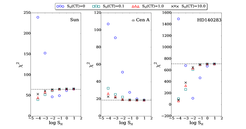
Figure 1: $\chi^{2}$ as a function of scaling factors S_H and S_H(CT) for the Sun, HD140283 and $\alpha$ Cen A. The dotted lines represent the $\chi^{2}$ values obtained in LTE.

For the Sun, it can be seen that when charge transfer rates are neglected, the best fit is obtained at S_H=0.01. Upon including charge transfer rates, smaller S_H values are needed. For the metal-rich star $\alpha$ Cen A, larger values of S_H and S_H(CT) are favored. For the metal-poor star HD140283, large variations in $\chi^{2}$ are obtained with S_H and S_H(CT) showing that charge transfer process plays an important role in producing the best-fit. Similar to the Sun, the best fit is also obtained at S_H=0.01 upon neglecting the charge transfer rates, while smaller values of S_H are needed when including them.

Comparing to recent studies, Mashonkina et al. (2011) and Bergemann et al. (2012) used Fe I/Fe II model atoms in their non-LTE abundance determinations, which are comparable to our model. Their calculations were also tested on benchmark stars including the Sun and HD140283, where they used the Drawin approximation scaled with an S_H-factor for the excitation and ionization H collisional rates. Charge transfer rates were not included in their calculations. They could not find a single S_H-factor that would fit all stars. For metal-poor stars, Mashonkina et al. (2011) determined a value of S_H=0.1 while Bergemann et al. (2012) determined an optimum value of S_H=1. For solar-metallicity stars, both studies found that different S_H values had no significant effect on the calculated abundances.

Similarly, we could not find a single set of S_H values that would ensure a best fit for all stars. We could, however, note that including charge transfer H collisional rates is important in iron non-LTE calculations. When neglecting charge transfer rates, however, a large value of S_H is needed for $\alpha$ Cen A (S_H $>$ 1), while a smaller value is needed for the Sun and HD140283 (S_H $\leq$ 0.01), which is not in accordance with previous studies.

4 Conclusions

We performed iron non-LTE spectral line calculations for three benchmark stars with well determined atmospheric parameters, using hydrogen collisions for excitation and ionization processes, and including charge transfer rates for the first time. We show that the charge transfer rates are important to include in the non-LTE calculations, especially for the metal-poor star. They were found, however, to play a less important role with increasing metallicity for the Sun and the metal-rich star $\alpha$ Cen A, where non-LTE effects are of smaller magnitude. No single set of values for the scaling factors S_H and S_H(CT) was obtained for the different types of stars. This demonstrates the inability of the Drawin approximation to reproduce the correct behavior and magnitudes of hydrogen collision rates (see Barklem et al. (2011)). In the lack of quantum calculations for the hydrogen collision rates, more efficient models than the classical Drawin approximation are required. We are working on such a method based on semi-empirical fitting of the available quantum data for other chemical species.