Second Kind Integral Equation Formulation for the Mode Calculation of Optical Waveguides

Abstract

We present a second kind integral equation (SKIE) formulation for calculating the electromagnetic modes of optical waveguides, where the unknowns are only on material interfaces. The resulting numerical algorithm can handle optical waveguides with a large number of inclusions of arbitrary irregular cross section. It is capable of finding the bound, leaky, and complex modes for optical fibers and waveguides including photonic crystal fibers (PCF), dielectric fibers and waveguides. Most importantly, the formulation is well conditioned even in the case of nonsmooth geometries. Our method is highly accurate and thus can be used to calculate the propagation loss of the electromagnetic modes accurately, which provides the photonics industry a reliable tool for the design of more compact and efficient photonic devices. We illustrate and validate the performance of our method through extensive numerical studies and by comparison with semi-analytical results and previously published results.

Keywords:  Mode calculation, optical waveguide, optical fiber, hybrid mode, second kind integral equation formulation.

1 Introduction

Optical fibers and waveguides are important building blocks of many photonic devices and systems in telecommunication, data transfer and processing, and optical computing. Indeed, most photonic devices consist of approximately straight waveguides as input and output channels with complicated functional structures between the two. Two main mechanisms by which the electromagnetic wave can be confined in optical fibers or waveguides are total internal reflection and photonic band gap guidance [42, 23]. Generally speaking, when the refractive index of the core is greater than that of the surrounding material, the light is confined in the core by total internal reflection; when the (hollow) core has a smaller refractive index, confinement can be achieved through photonic band gap guidance. In both cases, the propagating electromagnetic modes of optical fibers and waveguides depend on physical parameters such as the input light wavelength, refractive indices, and the geometry of the cross section of fibers and waveguides. To reduce the cost of designing new photonic devices, accurate and efficient simulation tools are in high demand in integrated photonics industry. The first step in the photonics simulation is to compute a complete set of propagating modes accurately and efficiently for optical fibers or waveguides.

There has been extensive research on the mode calculation of optical fibers and waveguides and various numerical methods have been developed. These include the effective index method [38, 10], the plane wave expansion method [17, 48, 24], the multipole expansion method [53, 54, 32, 12, 11, 52, 30], finite difference methods [19, 50, 14, 56], finite element methods [4, 16, 26, 5, 45, 41, 44], boundary integral methods [51, 18, 33, 34, 13, 15, 3, 35, 36, 49, 43], etc. Here we do not intend to review these methods in great detail, but note that the effective index method is generally of low order making it difficult to calculate the propagation constant to high accuracy; the plane wave expansion method implies an infinite periodic medium; the multipole expansion method requires that each core be of circular shape and that the cores be well separated from each other; finite difference and finite element methods requires a volume discretization of the cross section in a truncated computational domain with some artificial boundary conditions or perfectly matched layers imposed on or near the boundary of the truncated domain. When optical fibers and waveguides consist of many cores of arbitrary shape, these methods often need excessively large amount of computing resource in order to accurately calculate the imaginary part of the propagation constant, which is related to the propagation loss of the electromagnetic modes and thus of fundamental importance for the design purpose.

On the other hand, boundary integral methods represent the electromagnetic fields via layer potentials which satisfy the underlying partial differential equations automatically. One then derives a set of integral equations through the matching of boundary conditions with the unknowns only on the material interfaces. Thus the dimension of the problem is reduced by one and complex geometries can be handled relatively easily. Among the aforementioned work on boundary integral methods, [13, 3, 35, 43] present numerical examples with high accuracy for smooth geometries. In [3] and [43], the field components $E_{z}$ and $H_{z}$ (with $z$-axis the longitudinal direction of the waveguide) are represented via four distinct single layer potentials and the resulting system is a mixture of first kind and singular integral equations; both authors apply the circular case as a preconditioner to obtain a well conditioned system for smooth boundaries. In [13], $E_{z}$ and $H_{z}$ are represented via a proper linear combination of single and double layer potentials in such a way that the hypersingular terms are cancelled out. The resulting system still contains the tangential derivatives of the unknown densities and layer potentials and thus is not of the second kind. In [35], Dirichlet-to-Neumann (DtN) maps for $H_{x}$ and $H_{y}$ are used to construct a system of two integral equations, where each DtN map is in turn computed by a boundary integral equation with a hypersingular integral operator and a method in [29] is applied to evaluate the DtN map to high accuracy for smooth boundaries. While these methods are all capable of computing the propagation constant to high accuracy for smooth cases, it is not straightforward to extend them to treat nonsmooth cases such as standard dielectric rectangular waveguides in integrated optics.

Remark 1

We would like to remark here that [3] has a subsection titled “Buried Rectangular Dielectric Waveguide”. In that subsection, the authors approximate the rectangular waveguide via a smooth super-ellipse and compute the propagation constant for the super-ellipse. Though Fig. 2 in [3] achieves about $9$ digit accuracy for the super-ellipse, Fig. 3 in [3] shows only about two digit accuracy for the propagation constant of the genuine rectangular waveguide which is regarded as a limit of the super-ellipse.

In this paper, we construct a system of SKIEs formulation for the mode calculation of optical waveguides. Our starting point is the dual Müller’s formulation [39] for the time-harmonic Maxwell’s equations in three dimensions. We then reduce the dimension of the integration domain by one using the key assumption of the mode calculation that the dependence on $z$ of the electromagnetic fields and the unknown densities is of the form $e^{i\beta z}$, where $\beta$ is the propagation constant of the mode. Accordingly, the layer potentials defined on the surface of the waveguide are reduced to the layer potentials defined only on the boundary of the cross section. And the boundary conditions lead to a system of four SKIEs where each integral equation consists of a sum of a constant multiple of the identity operator and several compact operators. All involved integral operators have logarithmically singular kernels and thus are straightforward to discretize with high order quadratures. Hence, our formulation leads to a numerical algorithm which can handle the mode calculation of optical waveguides of arbitrary geometries (smooth and nonsmooth) accurately and efficiently.

The paper is organized as follows. In Section 2, we develop the SKIE formulation. We discuss briefly the discretization scheme and numerical algorithm for the mode finding in Section 3. In Section 4, we illustrate the performance of our scheme numerically and compare our results with semi-analytical results or previously published results in [13, 35, 43] for PCFs with smooth holes. High accuracy results for dielectric rectangular waveguides are presented in Section 5. And concluding remarks are contained in Section 6.

2 SKIE formulation for the electromagnetic mode calculation

In this section, we first derive the SKIE formulation for the electromagnetic mode calculation when the waveguide consists of only one core. The extension to the case of multiple cores or holes is straightforward.

Figure 1: Cross section of an optical waveguide consisting of multiple cores

2.1 Notation

We follow standard conventions in the mode calculation literature and assume that electromagnetic fields are propagated along the $z$-axis, and that the geometric structure of the optical waveguides is completely determined by its cross section in the $xy$-plane (see Fig. 1 for an illustration). The waveguide consists of several cores (or holes) denoted by $\Omega_{1},\cdots,\Omega_{N}$ with refractive indices $n_{1},\cdots,n_{N}$, respectively. The surroundings of these cores or the cladding is denoted by $\Omega_{0}$ with refractive index $n_{0}$. The boundary of each core is denoted by $\Gamma_{i}$ with $\nu$ the unit outward normal vector and $\tau$ the unit tangential vector, respectively. We denote points in $\mathbb{R}^{2}$ by $P$ and $Q$.

2.2 PDE formulation

The source free Maxwell equations in each homogeneous region are given by:

$$\nabla\times\mathbf{E} = -\mu_{0}\frac{\partial\mathbf{H}}{\partial t},$$ (1)

$$\nabla\times\mathbf{H} = \epsilon_{0}n^{2}\frac{\partial\mathbf{E}}{\partial t},$$ (2)

$$\nabla\cdot\mathbf{E} = 0,$$ (3)

$$\nabla\cdot\mathbf{H} = 0,$$ (4)

where $n$ is the index of refraction of the region.

Assuming the time dependence of the electromagnetic field is $e^{-i\omega t}$, i.e., $\mathbf{E}(x,y,,t)=\mathbf{E}(x,y,z)e^{-i\omega t}$ and $\mathbf{H}(x,y,,t)=\mathbf{H}(x,y,z)e^{-i\omega t}$, and rescaling the magnetic field $\mathbf{H}$ by $\sqrt{\frac{\mu_{0}}{\epsilon_{0}}}$, equations (1)-(2) become

$$\nabla\times\mathbf{E}-ik_{v}\mathbf{H}=0,$$ (5)

$$\nabla\times\mathbf{H}+i\frac{k^{2}}{k_{v}}\mathbf{E}=0,$$ (6)

where $k=k_{v}n$ is the wave number in the region, $k_{v}=\omega/c$ is the wave number in vacuum, and $c=\frac{1}{\sqrt{\epsilon_{0}\mu_{0}}}$ is the speed of light in vacuum. In the mode calculation, a further important assumption is that the electromagnetic field takes the following form:

$$\mathbf{E}(x,y,z) = \mathbf{E}(x,y)e^{i\beta z},$$ (7)

$$\mathbf{H}(x,y,z) = \mathbf{H}(x,y)e^{i\beta z}.$$ (8)

We observe that with this assumption each component of the electromagnetic fields of the mode satisfies the Helmholtz equation in two dimensions:

$$\left[\Delta+(k^{2}-\beta^{2})\right]u=0.$$ (9)

On the material interface, the boundary conditions are that the tangential components of the electromagnetic fields are continuous. That is,

$$[\nu\times\mathbf{E}]=0,\qquad[\nu\times\mathbf{H}]=0,$$ (10)

where $[\cdot]$ denotes the jump across the material interface. It is clear that $z$ and $\tau$ are two tangential directions for the waveguide geometry. Thus the boundary conditions can be written explicitly as follows:

$$[E_{z}]=0,\qquad[E_{\tau}]=0,\qquad[H_{z}]=0,\qquad[H_{\tau}]=0.$$ (11)

Finally, we would like to remark that combining the assumptions (7), (8) and Maxwell’s equations, it is straightforward to verify that there are only two independent components for the electromagnetic fields in each region. For instance, the components $E_{x}$, $E_{y}$, $H_{x}$, $H_{y}$ are completely determined by $E_{z}$ and $H_{z}$ via the following relations:

$$\begin{bmatrix}H_{x}\\ E_{y}\end{bmatrix}=\frac{-1}{k^{2}-\beta^{2}}\begin{bmatrix}ik^{2}/k_{v}&-i\beta\\ -i\beta&ik_{v}\end{bmatrix}\begin{bmatrix}\frac{\partial E_{z}}{\partial y}\\ \frac{\partial H_{z}}{\partial x}\end{bmatrix}.$$ (12)

$$\begin{bmatrix}E_{x}\\ H_{y}\end{bmatrix}=\frac{1}{k^{2}-\beta^{2}}\begin{bmatrix}i\beta&ik_{v}\\ ik^{2}/k_{v}&i\beta\end{bmatrix}\begin{bmatrix}\frac{\partial E_{z}}{\partial x}\\ \frac{\partial H_{z}}{\partial y}\end{bmatrix}.$$ (13)

In fact, [13, 3, 43] start from the integral representation of $E_{z}$ and $H_{z}$ to develop the integral equation formulation for the mode calculation.

2.3 SKIE formulation

We first provide an informal description about our construction of the SKIE formulation for the mode calculation of optical waveguides. Previous integral equation formulations in [13, 3, 43, 35] start from two scalar variables, i.e., two components of the electromagnetic fields ($E_{z}$ and $H_{z}$ in [13, 3, 43] and $H_{x}$, $H_{y}$ in [35]) and then set up the integral equations through the boundary conditions. Here we start from the dual Müller’s representation in [39] for the time harmonic electromagnetic fields which leads to an SKIE formulation for the dielectric interface problems in three dimensions. As an integral representation for three dimensional problem, the integration domain is over the boundary $\partial\Omega$ and the unknowns are the surface currents $\mathbf{J}$ and $\mathbf{M}$ on $\partial\Omega$. For the mode calculation of an optical waveguide, the boundary is an infinitely long cylinder, i.e., $\partial\Omega=\Gamma\times(-\infty,\infty)$ where $\Gamma$ is the boundary of the cross section of the waveguide. Since all electromagnetic field components have $e^{i\beta z}$ dependence on $z$, it is natural to assume that the unknown surface currents $\mathbf{J}$ and $\mathbf{M}$ have the same dependence on $z$ as well. Combining these two factors, we are able to reduce the dimension of the representation by one and derive an integral representation of $\mathbf{E}(x,y)$ and $\mathbf{H}(x,y)$ using layer potentials defined only on $\Gamma$. It is readily to verify that the boundary conditions lead to a system of SKIEs for the mode calculation, with the propagation constant $\beta$ appearing as a nonlinear parameter of the system.

2.3.1 Reduction of layer potentials in the mode calculation

The dual Müller’s representation [39] assumes that in each region the time harmonic electromagnetic field $\mathbf{E}(x,y,z)$ and $\mathbf{H}(x,y,z)$ have the following representation:

$$\mathbf{E} = \frac{1}{ik_{v}}\nabla\times(\nabla\times S^{k}_{\partial\Omega}[\mathbf{J}])-\nabla\times S^{k}_{\partial\Omega}[\mathbf{M}],$$ (14)

$$\mathbf{H} = -\frac{1}{ik_{v}}\nabla\times(\nabla\times S^{k}_{\partial\Omega}[\mathbf{M}])-\frac{k^{2}}{k_{v}^{2}}\nabla\times S^{k}_{\partial\Omega}[\mathbf{J}].$$ (15)

Here $\partial\Omega$ is the boundary of the three dimensional domain, $\mathbf{J}$ and $\mathbf{M}$ are the unknown surface electric and magnetic currents, and

$$S^{k}_{\partial\Omega}[\mathbf{J}]({\mathbf{r}})=\frac{1}{4\pi}\int_{\partial\Omega}\frac{e^{ik|{\mathbf{r}}-{\mathbf{r}}^{\prime}|}}{|{\mathbf{r}}-{\mathbf{r}}^{\prime}|}\mathbf{J}({\mathbf{r}}^{\prime})d{\mathbf{r}}^{\prime}$$ (16)

is the single layer potential for the Helmholtz equation in 3D with similar expression for $S^{k}_{\partial\Omega}[\mathbf{M}]$. Obviously, $S^{k}_{\partial\Omega}[\mathbf{J}]$ satisfies the Helmholtz equation in 3D, i.e., $(\nabla^{2}+k^{2})S^{k}_{\partial\Omega}[\mathbf{J}]({\mathbf{r}})=0$ for ${\mathbf{r}}\in\Omega$. It is straightforward to verify that (14)-(15) satisfy Maxwell’s equations (3)-(6).

For the waveguide geometry, $\partial\Omega=\Gamma\times(-\infty,\infty)$. Furthermore, since both $\mathbf{E}(x,y,z)$ and $\mathbf{H}(x,y,z)$ depend on $z$ in the form of $e^{i\beta z}$, it is natural to assume that the surface currents $\mathbf{J}(x,y,z)$ and $\mathbf{M}(x,y,z)$ have the same $z$ dependence as well, that is,

$$\mathbf{J}(x,y,z)=\mathbf{J}(x,y)e^{i\beta z},\qquad\mathbf{M}(x,y,z)=\mathbf{M}(x,y)e^{i\beta z}.$$ (17)

We now introduce some notation to be used subsequently. We denote $k_{\beta}=\sqrt{k^{2}-\beta^{2}}$ and the Green’s function for the Helmholtz equation (9) in 2D by $G(P,Q)=\frac{i}{4}H^{(1)}_{0}(k_{\beta}|P-Q|)$, where $H^{(1)}_{0}$ is the zeroth order Hankel function of the first kind [1]. We further denote by $S$ the single layer potential operator defined by the formula

$$S[\sigma]=\int_{\Gamma}G(P,Q)\sigma(Q)ds_{Q};$$ (18)

$D$ the double layer potential operator defined by the formula

$$D[\sigma]=\int_{\Gamma}\frac{\partial G(P,Q)}{\partial\nu(Q)}\sigma(Q)ds_{Q};$$ (19)

and $T$ the anti-double layer potential operator (for the lack of standard terminology) defined by the formula

$$T[\sigma]=\int_{\Gamma}\frac{\partial G(P,Q)}{\partial\tau(Q)}\sigma(Q)ds_{Q}.$$ (20)

The following lemma shows that the Fourier transform of the 3D Helmholtz Green’s function is the 2D Helmholtz Green’s function.

Lemma 2.1

$$\int_{-\infty}^{\infty}\frac{1}{4\pi}\frac{e^{ik|{\mathbf{r}}-{\mathbf{r}}^{\prime}|}}{|{\mathbf{r}}-{\mathbf{r}}^{\prime}|}e^{i\beta z^{\prime}}dz^{\prime}=G(P,Q)e^{i\beta z},$$ (21)

where $P=(x,y)$ and $Q=(x^{\prime},y^{\prime})$ are the projections of ${\mathbf{r}}=(x,y,z)$ and ${\mathbf{r}}^{\prime}=(x^{\prime},y^{\prime},z^{\prime})$ onto the $xy$-plane, respectively, and the wavenumber $k_{\beta}$ in $G$ is chosen to have nonnegative imaginary part.

• Let $|P-Q|=\sqrt{(x-x^{\prime})^{2}+(y-y^{\prime})^{2}}=a$, and $t=z-z^{\prime}$. Then

  $$\frac{1}{4\pi}\int_{-\infty}^{\infty}\frac{e^{ik|{\mathbf{r}}-{\mathbf{r}}^{\prime}|}}{|{\mathbf{r}}-{\mathbf{r}}^{\prime}|}e^{i\beta z^{\prime}}dz^{\prime}=e^{i\beta z}\frac{1}{4\pi}\int_{-\infty}^{\infty}\frac{e^{ik\sqrt{a^{2}+t^{2}}}}{\sqrt{a^{2}+t^{2}}}e^{-i\beta t}dt$$ (22)

  We now note that the well-known Sommerfeld integral identity (for $y>0$) [47] is given by:

  $$\frac{i}{4}H_{0}^{1}(k_{s}\sqrt{x^{2}+y^{2}})=\frac{1}{4\pi}\int_{-\infty}^{\infty}\frac{e^{-\sqrt{\lambda^{2}-k_{s}^{2}}y}}{\sqrt{\lambda^{2}-k_{s}^{2}}}e^{i\lambda x}d\lambda.$$ (23)

  (21) follows from the substitution $\lambda=it$, $y=k$, $x=i\beta$ and $k_{s}=a$ and appropriate contour deformation.

The following corollary reduces the single layer potential $S^{k}_{\partial\Omega}$ in 3D to a single layer potential in 2D in the mode calculation of an optical waveguide.

Corollary 2.2

Suppose that $\partial\Omega=\Gamma\times(-\infty,\infty)$ and density $\sigma(x,y,z)=\mu(x,y)e^{i\beta z}$. Then

$$S^{k}_{\partial\Omega}[\sigma]({\mathbf{r}})=e^{i\beta z}S[\mu](P).$$ (24)

• $$S^{k}_{\partial\Omega}[\sigma]({\mathbf{r}}) =\int_{\Gamma}\mu(x^{\prime},y^{\prime})ds_{\Gamma}\int_{-\infty}^{\infty}\frac{1}{4\pi}\frac{e^{ik|{\mathbf{r}}-{\mathbf{r}}^{\prime}|}}{|{\mathbf{r}}-{\mathbf{r}}^{\prime}|}e^{i\beta z^{\prime}}dz^{\prime}$$ (25)

  $$=e^{i\beta z}\int_{\Gamma}\frac{i}{4}H^{(1)}_{0}(k_{\beta}|P-Q|)\mu(Q)ds_{Q}$$

  $$=e^{i\beta z}S[\mu](P),$$

  where the second equality follows from (21).

2.3.2 Integral representations of the electromagnetic field in the mode calculation

Let $(\hat{i},\hat{j},\hat{k})$ be the basis of the Cartesian coordinate with $\hat{k}$ pointing along the positive $z$ direction. We write the unit tangent vector in its component form $\tau=\tau_{1}\hat{i}+\tau_{2}\hat{j}$. Then the outward unit normal vector $\nu$ is given by $\nu=\nu_{1}\hat{i}+\nu_{2}\hat{j}=\tau_{2}\hat{i}-\tau_{1}\hat{j}$. Since $\mathbf{J}$ and $\mathbf{M}$ are unknown surface currents and $\tau$, $\hat{k}$ are two locally orthonormal tangential vectors at a point $(x,y,z)\in\partial\Omega$, we may write $\mathbf{J}(x,y)$ and $\mathbf{M}(x,y)$ in (17) for $(x,y)\in\Gamma$ as follows:

$$\mathbf{J}(x,y) =J_{\tau}(x,y)\tau+J_{z}(x,y)\hat{k}=J_{\tau}\tau_{1}\hat{i}+J_{\tau}\tau_{2}\hat{j}+J_{z}\hat{k},$$ (26)

$$\mathbf{M}(x,y) =M_{\tau}(x,y)\tau+M_{z}(x,y)\hat{k}=M_{\tau}\tau_{1}\hat{i}+M_{\tau}\tau_{2}\hat{j}+M_{z}\hat{k}.$$

We now write down our integral representations for the electromagnetic field in each region in the mode calculation of optical waveguides.

Theorem 2.3 (Integral representations of the electromagnetic field)

Suppose that the unknown surface currents $\mathbf{J}(x,y,z)$ and $\mathbf{M}(x,y,z)$ are given in the form of (17) and (26). Then $\mathbf{E}(x,y,z)$ defined in (14) has the form $\mathbf{E}(x,y,z)=(E_{x}(x,y),E_{y}(x,y),E_{z}(x,y))e^{i\beta z}$, where $E_{x}$, $E_{y}$ and $E_{z}$ are defined via the formulas:

$$E_{x} =-\frac{1}{ik_{v}}\frac{\partial}{\partial x}T[J_{\tau}]+\frac{\beta}{k_{v}}\frac{\partial}{\partial x}S[J_{z}]+\frac{k^{2}}{ik_{v}}S[J_{\tau}\tau_{1}]-\frac{\partial}{\partial y}S[M_{z}]+i\beta S[M_{\tau}\tau_{2}],$$ (27)

$$E_{y} =-\frac{1}{ik_{v}}\frac{\partial}{\partial y}T[J_{\tau}]+\frac{\beta}{k_{v}}\frac{\partial}{\partial y}S[J_{z}]+\frac{k^{2}}{ik_{v}}S[J_{\tau}\tau_{2}]+\frac{\partial}{\partial x}S[M_{z}]-i\beta S[M_{\tau}\tau_{1}],$$

$$E_{z} =-\frac{\beta}{k_{v}}T[J_{\tau}]+\frac{(k^{2}-\beta^{2})}{ik_{v}}S[J_{z}]+D[M_{\tau}].$$

Similarly, $\mathbf{H}(x,y,z)=(H_{x}(x,y),H_{y}(x,y),H_{z}(x,y))e^{i\beta z}$, where $H_{x}$, $H_{y}$ and $H_{z}$ are defined via the formulas:

$$H_{x} =\frac{1}{ik_{v}}\frac{\partial}{\partial x}T[M_{\tau}]-\frac{\beta}{k_{v}}\frac{\partial}{\partial x}S[M_{z}]-\frac{k^{2}}{ik_{v}}S[M_{\tau}\tau_{1}]-\frac{k^{2}}{k_{v}^{2}}\frac{\partial}{\partial y}S[J_{z}]+i\beta\frac{k^{2}}{k_{v}^{2}}S[J_{\tau}\tau_{2}],$$ (28)

$$H_{y} =\frac{1}{ik_{v}}\frac{\partial}{\partial y}T[M_{\tau}]-\frac{\beta}{k_{v}}\frac{\partial}{\partial y}S[M_{z}]-\frac{k^{2}}{ik_{v}}S[M_{\tau}\tau_{2}]+\frac{k^{2}}{k_{v}^{2}}\frac{\partial}{\partial x}S[J_{z}]-i\beta\frac{k^{2}}{k_{v}^{2}}S[J_{\tau}\tau_{1}],$$

$$H_{z} =\frac{\beta}{k_{v}}T[M_{\tau}]-\frac{(k^{2}-\beta^{2})}{ik_{v}}S[M_{z}]+\frac{k^{2}}{k_{v}^{2}}D[J_{\tau}].$$

• By Corollary 2.2, we have

  $$S^{k}_{\partial\Omega}[\mathbf{J}]=e^{i\beta z}S[\mathbf{J}],\qquad S^{k}_{\partial\Omega}[\mathbf{M}]=e^{i\beta z}S[\mathbf{M}].$$ (29)

  Thus,

  $$S^{k}_{\partial\Omega}[\mathbf{J}]=e^{i\beta z}\left(S[J_{\tau}\tau_{1}]\hat{i}+S[J_{\tau}\tau_{2}]\hat{j}+S[J_{z}]\hat{k}\right)$$ (30)

  and similar expression holds for $S^{k}_{\partial\Omega}[\mathbf{M}]$. Since

  $$\nabla\times S^{k}_{\partial\Omega}[\mathbf{J}] =e^{i\beta z}\left\{\left(\frac{\partial}{\partial y}S[J_{z}]-i\beta S[J_{\tau}\tau_{2}]\right)\hat{i}\right.$$ (31)

  $$+\left(-\frac{\partial}{\partial x}S[J_{z}]+i\beta S[J_{\tau}\tau_{1}]\right)\hat{j}$$

  $$+\left.\left(\frac{\partial}{\partial x}S[J_{\tau}\tau_{2}]-\frac{\partial}{\partial y}S[J_{\tau}\tau_{1}]\right)\hat{k}\right\}$$

  and

  $$\frac{\partial}{\partial x}S[J_{\tau}\tau_{2}]-\frac{\partial}{\partial y}S[J_{\tau}\tau_{1}]$$ (32)

  $$\ =-\int_{\Gamma}\frac{\partial G(P,Q)}{\partial x^{\prime}}J_{\tau}(Q)\tau_{2}(Q)ds_{Q}+\int_{\Gamma}\frac{\partial G(P,Q)}{\partial y^{\prime}}J_{\tau}(Q)\tau_{1}(Q)ds_{Q}$$

  $$\ =-\int_{\Gamma}\frac{\partial G(P,Q)}{\partial x^{\prime}}J_{\tau}(Q)\nu_{1}(Q)ds_{Q}-\int_{\Gamma}\frac{\partial G(P,Q)}{\partial y^{\prime}}J_{\tau}(Q)\nu_{2}(Q)ds_{Q}$$

  $$=-\int_{\Gamma}\frac{\partial G(P,Q)}{\partial\nu(Q)}J_{\tau}(Q)ds_{Q}=-D[J_{\tau}](P),$$

  we have

  $$\nabla\times S^{k}_{\partial\Omega}[\mathbf{J}] =e^{i\beta z}\left\{\left(\frac{\partial}{\partial y}S[J_{z}]-i\beta S[J_{\tau}\tau_{2}]\right)\hat{i}\right.$$ (33)

  $$\left.+\left(-\frac{\partial}{\partial x}S[J_{z}]+i\beta S[J_{\tau}\tau_{1}]\right)\hat{j}-D[J_{\tau}]\hat{k}\right\}.$$

  Using the identity $\nabla\times(\nabla\times\mathbf{A})=\nabla(\nabla\cdot\mathbf{A})-\nabla^{2}\mathbf{A}$, we have

  $$\nabla\times(\nabla\times S^{k}_{\partial\Omega}[\mathbf{J}]) =\nabla(\nabla\cdot S^{k}_{\partial\Omega}[\mathbf{J}])-\nabla^{2}S^{k}_{\partial\Omega}[\mathbf{J}]$$ (34)

  $$=\nabla(\nabla\cdot S^{k}_{\partial\Omega}[\mathbf{J}])+k^{2}S^{k}_{\partial\Omega}[\mathbf{J}]$$

  $$=\nabla(\nabla\cdot(e^{i\beta z}S[\mathbf{J}]))+k^{2}e^{i\beta z}S[\mathbf{J}],$$

  and

  $$\nabla\cdot(e^{i\beta z}S[\mathbf{J}]) =e^{i\beta z}\left(\frac{\partial}{\partial x}S[J_{\tau}\tau_{1}]+\frac{\partial}{\partial y}S[J_{\tau}\tau_{2}]+i\beta S[J_{z}]\right)$$ (35)

  $$=e^{i\beta z}\left(-T[J_{\tau}]+i\beta S[J_{z}]\right).$$

  Thus,

  $$\nabla(\nabla\cdot(e^{i\beta z}S[\mathbf{J}]) =e^{i\beta z}\left\{\left(-\frac{\partial}{\partial x}T[J_{\tau}]+i\beta\frac{\partial}{\partial x}S[J_{z}]\right)\hat{i}\right.$$ (36)

  $$+\left(-\frac{\partial}{\partial y}T[J_{\tau}]+i\beta\frac{\partial}{\partial y}S[J_{z}]\right)\hat{j}$$

  $$\left.+\left(-i\beta T[J_{\tau}]-\beta^{2}S[J_{z}]\right)\hat{k}\right\}.$$

  Substituting (30), (33) (with $\mathbf{J}$ replaced by $\mathbf{M}$), (34), (36) into (14), we obtain (27). And (28) can be obtained similarly.

Remark 2

Though $\beta$ is assumed to be real in Lemme 2.1, we will use (27)-(28) to represent the electromagnetic field even when $\beta$ is complex for the mode calculation. In fact, it is straightforward (though a little tedious) to verify (27)-(28) satisfy the relations (12)-(13) even when $\beta$ is complex. The hard part is to verify the following identities:

$$\frac{\partial}{\partial y}T[M_{\tau}]+\frac{\partial}{\partial x}D[M_{\tau}] =-\nabla^{2}S[M_{\tau}\tau_{2}]=(k^{2}-\beta^{2})S[M_{\tau}\tau_{2}],$$ (37)

$$-\frac{\partial}{\partial x}T[J_{\tau}]+\frac{\partial}{\partial y}D[J_{\tau}] =\nabla^{2}S[J_{\tau}\tau_{1}]=-(k^{2}-\beta^{2})S[J_{\tau}\tau_{1}],$$

and other similar identities. In other words, we might start directly from the representation (27)-(28) for the mode calculation without even mentioning the dual Müller’s representation, which only serves as a formal derivation tool.

2.3.3 Main theoretical result

We are now in a position to derive the SKIE formulation for the mode calculation of photonic waveguides. Since the boundary conditions for dielectric problems are that the tangential components of $\mathbf{E}$ and $\mathbf{H}$ must be continuous across the boundary. We first combine the first two equations in (27) and (28) to obtain $E_{\tau}$ and $H_{\tau}$. Together with $E_{z}$ and $H_{z}$, we list all four tangential components as follows:

$$H_{z} =\frac{k^{2}}{k_{v}^{2}}D[J_{\tau}]+\frac{\beta}{k_{v}}T[M_{\tau}]+\frac{i(k^{2}-\beta^{2})}{k_{v}}S[M_{z}],$$ (38)

$$H_{\tau}(P) =i\beta\frac{k^{2}}{k_{v}^{2}}S[J_{\tau}(Q)\tau(P)\cdot\nu(Q)](P)+\frac{k^{2}}{k_{v}^{2}}S_{\nu}[J_{z}](P)$$

$$+i\frac{k^{2}}{k_{v}}S[M_{\tau}(Q)\tau(P)\cdot\tau(Q)](P)-\frac{i}{k_{v}}T_{\tau}[M_{\tau}](P)-\frac{\beta}{k_{v}}S_{\tau}[M_{z}](P),$$

$$E_{z} =-\frac{\beta}{k_{v}}T[J_{\tau}]-\frac{i(k^{2}-\beta^{2})}{k_{v}}S[J_{z}]+D[M_{\tau}],$$

$$E_{\tau}(P) =-\frac{ik^{2}}{k_{v}}S[J_{\tau}(Q)\tau(P)\cdot\tau(Q)](P)+\frac{i}{k_{v}}T_{\tau}[J_{\tau}](P)+\frac{\beta}{k_{v}}S_{\tau}[J_{z}](P)$$

$$+i\beta S[M_{\tau}(Q)\tau(P)\cdot\nu(Q)](P)+S_{\nu}[M_{z}](P).$$

We now scale and nondimensionalize the quantities in the above equation by multiplying all length quantities with $k_{v}$. We have

$$\tilde{H}_{z} =n^{2}D[J_{\tau}]+n_{e}T[M_{\tau}]+i(n^{2}-n_{e}^{2})S[M_{z}],$$ (39)

$$-\tilde{H}_{\tau}(P) =-in^{2}n_{e}S[J_{\tau}(Q)\tau(P)\cdot\nu(Q)](P)-n^{2}S_{\nu}[J_{z}](P)$$

$$-in^{2}S[M_{\tau}(Q)\tau(P)\cdot\tau(Q)](P)+iT_{\tau}[M_{\tau}](P)+n_{e}S_{\tau}[M_{z}](P),$$

$$\tilde{E}_{z} =-n_{e}T[J_{\tau}]-i(n^{2}-n_{e}^{2})S[J_{z}]+D[M_{\tau}],$$

$$-\tilde{E}_{\tau}(P) =in^{2}S[J_{\tau}(Q)\tau(P)\cdot\tau(Q)](P)-iT_{\tau}[J_{\tau}](P)-n_{e}S_{\tau}[J_{z}](P)$$

$$-in_{e}S[M_{\tau}(Q)\tau(P)\cdot\nu(Q)](P)-S_{\nu}[M_{z}](P),$$

where $n_{e}=\beta/k_{v}$ is the effective index.

For each region $\Omega_{i}$ ($i=0,1$ for now), we denote the single, double, and anti-double layer potential operators in that region by $S_{i}$, $D_{i}$, and $T_{i}$, respectively. We now summarize our main theoretical result in the following theorem.

Theorem 2.4 (SKIE formulation for the mode calculation)

Suppose that $\mathbf{E}(x,y)$ and $\mathbf{H}(x,y)$ in each region $\Omega_{i}$ ($i=0,1$) are represented via (27)-(28) with $k$, $S$, $D$, $T$ replaced by $k_{i}$, $S_{i}$, $D_{i}$, $T_{i}$, respectively. Then the densities $\mathbf{J}(x,y)$ and $\mathbf{M}(x,y)$ defined in (26) satisfy the following (nondimensionalized) system of second kind integral equations:

$$(D+A(n_{e}))x=0,$$ (40)

where $x=[J_{\tau}\ J_{z}\ M_{\tau}\ M_{z}]^{T}$ is a $4\times 1$ block vector, $D$ and $A$ are $4\times 4$ block matrices defined by the formulas

$$D=\begin{bmatrix}&\frac{n_{0}^{2}+n_{1}^{2}}{2}&&&&\\ &&\frac{n_{0}^{2}+n_{1}^{2}}{2}&&&\\ &&&1&&\\ &&&&1&\end{bmatrix},\quad A(n_{e})=\begin{bmatrix}&A_{11}&0&A_{13}&A_{14}&\\ &A_{21}&A_{22}&A_{23}&A_{24}&\\ &-A_{13}&-A_{14}&A_{33}&0&\\ &-A_{23}&-A_{24}&A_{43}&A_{44}&\end{bmatrix}.$$ (41)

Here the nonzero entries of $A$ are given by the following formulas:

$$A_{11} =n_{0}^{2}D_{0}-n_{1}^{2}D_{1},\qquad A_{22}=-n_{0}^{2}S_{0,\nu}+n_{1}^{2}S_{1,\nu},$$ (42)

$$A_{33} =D_{0}-D_{1},\qquad A_{44}=-S_{0,\nu}+S_{1,\nu},$$

$$A_{21} =-in_{e}\left(n_{0}^{2}S_{0}-n_{1}^{2}S_{1}\right)[\tau(P)\cdot\nu(Q)\cdot],$$

$$A_{43} =-in_{e}(S_{0}-S_{1})[\tau(P)\cdot\nu(Q)\cdot],$$

$$A_{13} =n_{e}(T_{0}-T_{1}),\qquad A_{24}=n_{e}\left(S_{0,\tau}-S_{1,\tau}\right),$$

$$A_{14} =i\left((n_{0}^{2}-n_{e}^{2})S_{0}-(n_{1}^{2}-n_{e}^{2})S_{1}\right),$$

$$A_{23} =i(T_{0,\tau}-T_{1,\tau})-i(n_{0}^{2}S_{0}-n_{1}^{2}S_{1})[\tau(P)\cdot\tau(Q)\cdot].$$

The effective index $n_{e}=\beta/k_{v}$ of the electromagnetic mode is a complex number for which the above linear system has a nontrivial solution.

• We first obtain the nondimensionalized tangential components in $\Omega_{i}$ ($i=0,1$) by replacing $n$, $S$, $D$, $T$ in (39) with $n_{i}$, $S_{i}$, $D_{i}$, $T_{i}$, respectively. We then substitute the resulting expressions into the boundary conditions (11) and observe that the principal part of the linear system is exactly the matrix $A$ defined in (41)-(42).

  It is easy to see now that only $D$ and $S_{\nu}$ have nonzero jumps when the target point $P$ approaches the boundary and their jump relations lead to the diagonal matrix $D$ in (41) (see, for example, [27]). Furthermore, all entries $A_{ij}$ are compact operators due to following reasons. First, $S$, and the principal part of $D$ and $S_{\nu}$ are compact from standard potential theory [27]. Second, $T_{0}-T_{1}$ and $S_{0,\tau}-S_{1,\tau}$ are compact since their kernels are only logarithmically singular due to the cancellation of more singular terms. Third, $T_{0,\tau}-T_{1,\tau}$ is also compact since the hypersingular terms in difference kernel cancel out. Thus, the resulting system is of the second kind.

2.4 Extension to the waveguide with multiple holes

When the waveguide consists of multiple holes, say, $\Omega_{1},\cdots,\Omega_{N}$, we simply represent $\mathbf{E}(x,y)$ and $\mathbf{H}(x,y)$ in each region $\Omega_{i}$ ($i=1,\cdots,N$) via (27)-(28) with $k$, $S$, $D$, $T$, $\Gamma$ replaced by $k_{i}$, $S_{i}$, $D_{i}$, $T_{i}$, $\Gamma_{i}$, respectively. For the exterior domain $\Omega_{0}$, we have similar representations for $\mathbf{E}(x,y)$ and $\mathbf{H}(x,y)$, except that the boundary $\Gamma$ is replaced by $\Gamma_{0}=\Gamma_{1}\cup\cdots\cup\Gamma_{N}$. The boundary conditions on each $\Gamma_{i}$ lead to a $4N\times 4N$ block system. We note that all $4\times 4$ diagonal blocks are similar to (40)-(42) and that the entries in off-diagonal blocks are all compact operators since their kernels are smooth due to the fact that the target point $P$ is bounded away from the source curve. Thus, the system is of the second kind.

3 Discretization and numerical algorithms

As pointed out in Theorem 2.4, all the integral operators in (40)-(42) have kernels with logarithmic singularity. When the boundary curves are smooth, there are many high-order quadrature rules based on local modifications of the trapezoidal rule [2, 25] or kernel splitting method [46, 28]. When the boundary curves contain corners, recent developments in [21, 20, 22, 6, 8, 9] treat such cases with high order quadratures very efficiently. In order to achieve optimal efficiency in discretization, one should treat smooth and nonsmooth cases separately and implement the aforementioned schemes (say, [2, 9]) accordingly.

Here we adopt a simpler scheme to discretize both smooth and nonsmooth cases. We divide the boundary curve into $N_{c}$ chunks as follows. If the curve is smooth, the chunks are of equal length in the parameter space. If the curve contains corners, we will have finer and finer dyadic chunks toward the corner. On each chunk, the unknown densities are approximated via a $p-1$th order polynomial and the set of collocation points are the collection of the images of $p$ shifted and scaled Gauss-Legendre nodes on each chunk. When the target points and the source points lie on the same chunk, we apply a precomputed generalized Gaussian quadrature (see, for example, [7, 37, 55]) to discretize the associated (logarithmically) singular integrals; and when the target points lie outside the integration chunk, we simply use an adaptive Gaussian integrator to compute the corresponding matrix entries. The total number of discretization points is $N=N_{c}p$, where $N_{c}$ is the number of chunks, and the size of the resulting matrix $M(n_{e})$ is $4N\times 4N$.

We apply the same method as in [13] to find the effective index $n_{e}$ such that $M(n_{e})$ has a nontrivial nullspace. That is, we use Müller’s method [40] to find the root of the function

$$f(n_{e})=\frac{1}{u^{T}M^{-1}(n_{e})v},$$ (43)

where $u$ and $v$ are two fixed random column vector of length $4N$.

4 Numerical examples for smooth boundaries

4.1 Example 1: optical fiber with a circular core

For our first example, we consider the silica optical fiber consisting of a single circular core of radius $50\mu m$. At the incident wavelength $\lambda=1500nm$, the refractive index of the core is $n_{1}=1.4475$ while that of the cladding is $n_{0}=1.444$. The effective index can be calculated independently by the multipole method [31] and our SKIE formulation. For this simple case, the multipole method is semi-analytical and one only needs to solve a $4\times 4$ system to find the effective index every time. Thus its results can be taken as the reference values for comparison purpose. Table 1 presents the first five modes obtained by our formulation with $50$ discretization points of the boundary and by the multipole method, which shows IEEE double precision agreement of these two results. We would like to remark here that our algorithm already achieves $13$ digit accuracy with only $20$ discretization points.

$n_{e}$ by SKIE		Reference value
Real	Imaginary	Real	Imaginary
1.444873245456804	0	1.444873245456804	0
1.445573321563491	0	1.445573321563491	0
1.445671696122978	0	1.445671696122978	0
1.446222363089593	0	1.446222363089593	0
1.447115413503111	0	1.447115413503111	0

Table 1: Effective index of Example 1. The first column lists the values obtained by the SKIE formulation with $50$ discretization points of the circular boundary; while the second column lists the values obtained by the multipole method in [31].

4.2 Example 2: PCFs with a hexagon ring and its perturbation

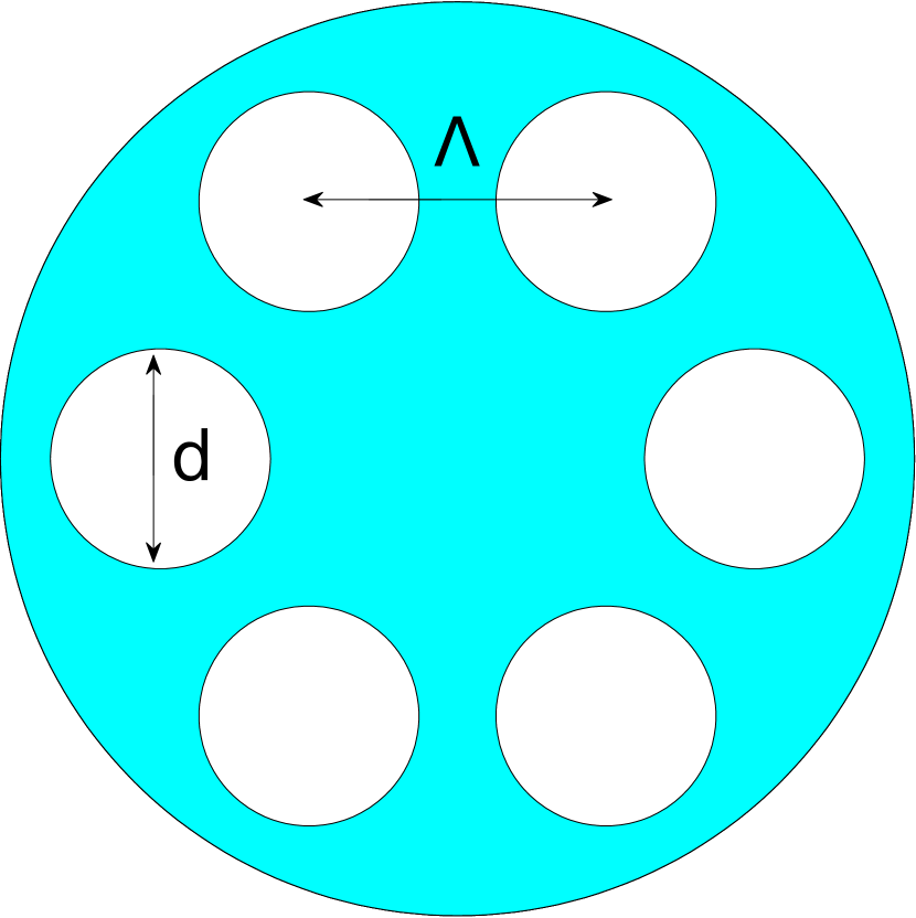
(a)

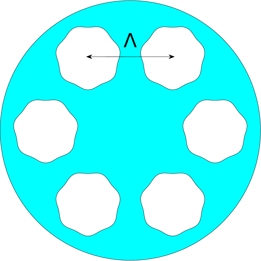
(b)

Figure 2: Geometry of the hexagon ring PCF (left panel) and its perturbation (right panel).

In this example, we consider two PCFs studied in [13] and [35]. The first PCF consists of a hexagon ring of circular air holes as shown in Figure 2(a). The six holes are equally spaced along the hexagon with hole diameter $d=5\mu m$ and hole pitch $\Lambda=6.75\mu m$. The refractive index of the glass matrix is assumed to be $n_{0}=1.45$ and that of the air hole is $1$. The incident wavelength is $1450nm$. The second PCF shown in Fig. 2(b) is the perturbation of the first one, where the holes have the parametrization:

$$||r(\theta)-c_{i}||=\frac{d}{2}(1+h\sin{7\theta})$$ (44)

Here $r(\theta)$ is the boundary of the $i$-th perturbed circle centered at $c_{i}$ and the perturbation level $h$ goes from $1\%$ to $6\%$.

We discretize each boundary curve by $100$ points. Table 2 lists the results obtained by our algorithm and the corresponding results in [13] for the first PCF. We observe that our algorithm is able to recover the first $10$ digits in [13] for all modes.

$n_{e}$		$n_{e}$ in [13]
Real	Imaginary	Real	Imaginary
1.44539523214929	3.19452506E-8	1.445395232	3.1945E-8
1.43858364729142	5.310787285E-7	1.438583647	5.3108E-7
1.43844483196668	9.730851491E-7	1.438444832	9.7308E-7
1.43836493417887	1.4164759939E-6	1.438364934	1.41647E-6
1.43040909603339	2.15661649916E-5	1.430409096	2.15662E-5
1.42995686266711	1.59153224394E-5	1.429956863	1.59153E-5
1.42924806251945	8.7312643348E-6	1.429248062	8.7313E-6

Table 2: Effective index of the PCF shown in Fig. 2(a).

Table 3 lists the results for the perturbed PCF. Compared with Table 2 in [13], we observe that the two results again have at least $10$ digit agreement with each other.

	$n_{e}$ for mode 1		$n_{e}$ for mode 2
h	Real	Imaginary	Real	Imaginary
1%	1.44539377438717	3.17269747E-8	1.44539377640333	3.17256375E-8
2%	1.44538941232987	3.10822988E-8	1.44538942033048	3.10770686E-8
3%	1.44538217911076	3.00407424E-8	1.44538219687975	3.00293984E-8
4%	1.44537215920563	2.86293848E-8	1.44537212816737	2.86485611E-8
5%	1.44535933076758	2.69649433E-8	1.44535937822583	2.69368186E-8
6%	1.44534387291222	2.50578633E-8	1.44534393955980	2.50203139E-8

Table 3: Effective index of the PCF shown in Fig. 2(b).

We have also studied the convergence rates for these two PCFs. The results are presented in Fig. 3, which shows the rapid convergence of our method.

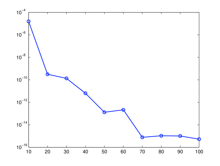
(a)

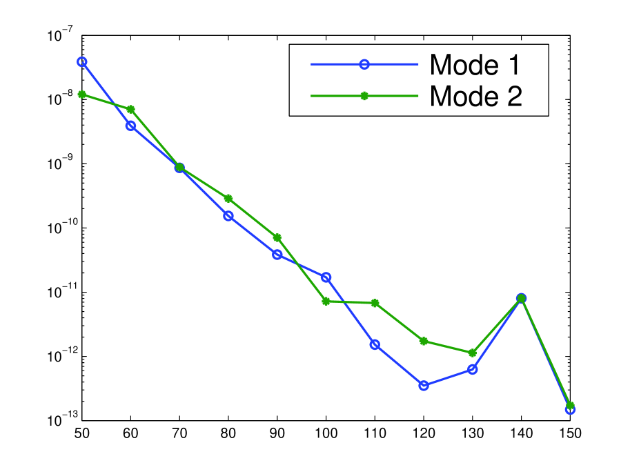
(b)

Figure 3: Convergence study of the PCFs shown in Fig. 2. The $x$ axis shows the number of discretization points for each hole and the $y$ axis shows the relative error of the computed effective index. The reference value is obtained with $200$ points on each hole boundary.

4.3 Example 3: PCFs with multiple-layer hexagon rings

We now consider PCFs with multiple layers. The examples are taken from [35, 43]. The first PCF has five layers of hexagon rings surrounding a circular core as shown in Figure 4(a). The small air holes are equally spaced with the hole pitch $\Lambda=2.74\mu m$ and the diameter $d=0.95\Lambda$. The diameter of the core is $l=2.5d$. The refractive indices of the glass surroundings and the air hole are $1.45$ and $1$, respectively. The wavelength of the incident field is $1510nm$. The second PCF has an elliptic core with minor axis $2a=2.3\mu m$ and major axis $2b=4.6\mu m$ surrounded by a three layers of hexagon rings. The hole pitch of the small air holes is $\Lambda=2\mu m$ and the diameter of each hole is $d=0.9\Lambda$. The incident wavelength for the second PCF is $\lambda=1420nm$. These two PCFs are shown in Fig. 4.

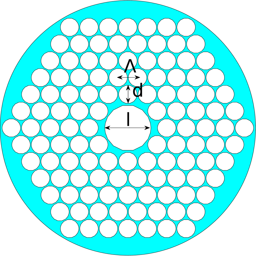
(a)

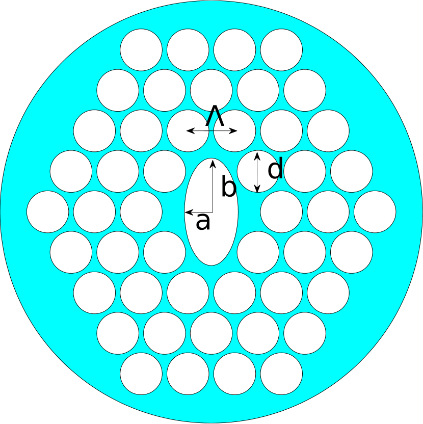
(b)

Figure 4: Geometry of two PCFs. For the PCF shown in the left panel, parameters are given by $\Lambda=2.74\mu m$, $d=0.95\Lambda$, $l=2.5d$. For the PCF shown in the right panel (b), parameters are given by $\Lambda=2\mu m$, $d=0.9\Lambda$, $a=1.15\mu m$, $b=2.3\mu m$.

The results of our computation for these two PCFs are shown in Table 4. For comparison, we also list the corresponding results in [35] in columns 4 and 5. The results in [35] are seen to be very accurate and there is a $13$ digit agreement between our results and the results in [35]. For the first PCF shown in Fig. 4(a), we discretize each small hole with $100$ points and the center hole with $200$ points; while for the second PCF shown in Fig. 4(b), we discretize each circular hole with $120$ points and the center ellipse with $240$ points.

	$n_{e}$		$n_{e}$ in [35]
	Real	Imaginary	Real	Imaginary
4(a)	0.9845160008345	3.41146823E-8	0.984516000835	3.41147E-8
4(b)	0.9390335474112	6.7418067299E-4	0.9390335474115	6.741806730E-4
	0.9381625147574	2.2133063780E-3	0.9381625147578	2.213306378E-3

Table 4: Effective index of the PCFs shown in Fig. 4. The second and third columns list the values obtained by our method and the last two columns list the values in [35].

5 Rectangular waveguides

In this section, we present a detailed numerical study on a high refractive index contrast silica waveguide. The cross section of the waveguide is of the square shape with the side length equal to $3.4\mu m$. The refractive index of the cladding is $n_{0}=1.4447$, while that of the core is $2\%$ higher, i.e., $n_{1}=1.4447\times 1.02$. The wavelength of the incident field is $1550nm$.

5.1 Accuracy and conditioning of the SKIE formulation

We first check the accuracy and conditioning of the SKIE formulation. For this, we will solve the linear system $M(n_{e})x=b$ with a nonzero right hand side for some $n_{e}\in[n_{0},n_{1}]$. We set $n_{e}=1.451$ for testing purpose and we construct artificial electromagnetic field by placing a point source outside the square for the interior field and a point source inside the square for the exterior field. We then obtain the right hand side vector $b$ by simply computing the difference of the tangential components of these artificial electromagnetic fields. After we have solved the linear system, we may use the representation (27)-(28) to evaluate the electromagnetic field both inside and outside and compare the numerical result with the exact solution (which is the artificial electromagnetic field by construction). We use GMRES to solve the linear system and GMRES terminates when the relative residual is less than $10^{-14}$.

$N$	150	300	450	600	750
$N_{\text{iter}}$	32	32	32	34	34

Table 5: Conditioning study of the SKIE formulation for the rectangular waveguide.

In Table 5, the first row lists the number of discretization points on each side of the square, while the second row lists the number of iterations needed in GMRES. We observe that the number of iterations in GMRES is almost independent of the size of the linear system, which is a characteristics of the SKIE formulation.

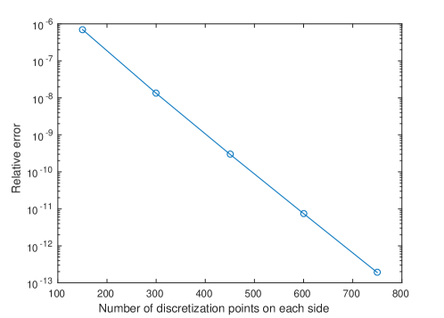
Figure 5: Convergence study of the rectangular waveguide. x-axis shows the number of discretization points on each side of the square; y-axis shows the relative error (in logarithmic scale) of the computed electromagnetic field against the exact value.

Figure 5 shows the relative error with various number of discretization points for each side of the square. We observe that the order of convergence is about $10$, which is in agreement with the theoretical value since the number of collocation points on each chunk is set to $p=10$.

5.2 Computation of the effective index

It is known that this waveguide admits a single propagation constant (or effective index) with double degeneracy. The method in [38] produces an effective index approximately equal to $1.458\cdots$. For comparison purpose, we have also implemented the formulation in [3, 43] which uses four distinct single layer potentials for the electromagnetic fields.

	$n_{e}$ by SREP		$n_{e}$ by SKIE
N	Real	Imaginary	Real	Imaginary
150	1.45867110663907	3E-10	1.45860141500175	3E-9
300	1.45884317112249	-2E-10	1.45860141488787	6E-11
450	1.45890000315967	9E-14	1.45860141488572	1E-12
600	1.45887005720651	-7E-6	1.45860141488567	3E-14

Table 6: Effective index of the rectangular waveguide. The first column lists the number of discretization points on each side of the square; the second and third columns list the real and imaginary parts of the effective index found via the formulation in [3, 43]; the fourth and fifth columns list the real and imaginary parts of the effective index found via our SKIE formulation.

Table 6 shows the effective index $n_{e}$ found by the formulation in [3, 43] (denoted by SREP in the table) and by our SKIE formulation for various number of discretization points. We observe that while the SKIE formulation exhibits a consistent convergence behavior to about $13$ digit accuracy as $N$ increases, the single layer representation behaves much more erratically and achieves about only $4$ digit accuracy. This is because that the resulting matrix from the discretization of the single layer representation becomes more and more ill-conditioned as $N$ increases even when $n_{e}$ is sufficiently far away from the root of the function defined in (43).

$N$	150	300	450	600
$\kappa_{\text{SREP}}$	4.8E+5	3.4E+7	2.0E+9	1.0E+10

Table 7: Condition number of the formulation in [3, 43] for the rectangular waveguide. The first row lists the number of discretization points on each side of the square, while the second row lists the condition number of the resulting matrix. $n_{e}$ is set to $1.451$ as in Table 5.

Table 7 lists the condition numbers of the matrix $M_{\text{SREP}}$ for various number of discretization points, which shows that the condition number of the matrix increases very rapidly even when $n_{e}$ is sufficiently far away from the root of the function in (43).

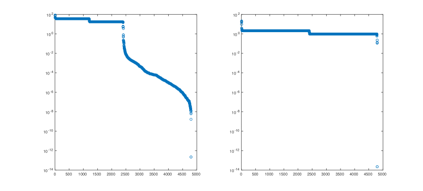
Figure 6: Singular value distribution of the matrices. The left panel shows the singular values of $M_{\text{SREP}}(n_{e})$ when the size of the matrix is $4800$ and $n_{e}=1.45884317112249-2E-10i$; while the right panel shows the singular values of $M_{\text{SKIE}}(n_{e})$ when the size of the matrix is $4800$ and $n_{e}=1.45860141488787+6E-11i$.

We have also carried out the singular value decomposition (SVD) for the matrices $M_{\text{SREP}}$ and $M_{\text{SKIE}}$ at the effective indices listed in Table 6 for $N=300$. The singular values are plotted out in Figure 6. We observe that the SKIE formulation has much cleaner singular value distribution. Indeed, the smallest two singular values are both about $2.2\times 10^{-14}$, while the third smallest singular value is about $0.1096$. On the other hand, the singular values of $M_{\text{SREP}}$ decreases almost continuously; the smallest two singular values are about $2\times 10^{-13}$, while the third smallest singular value is about $1.6\times 10^{-9}$. To sum up, the SKIE formulation enables us to find the effective index accurately and robustly; while non-SKIE formulation will either give low accuracy or lead to spurious propagation mode due to ill-conditioning.

6 Conclusions

We have constructed a second kind integral equation formulation for the mode calculation of optical waveguides or fibers. The resulting numerical algorithm is capable of finding the propagation modes of optical waveguides or fibers with an arbitrary number of cores or holes of arbitrary shape (smooth or with corners). The algorithm is high order accurate so that it is capable of computing the propagation constant (including its imaginary part which is related to the propagation loss of the mode) with high fidelity. The algorithm is robust and well-conditioned due to its SKIE formulation. The algorithm is efficient since one only needs to discretize the material interfaces. This enables practitioners in the integrated photonics industry to have a reliable simulation tool for designing more compact and efficient optical components or devices.

References

- [1] M. Abramowitz and I. A. Stegun, Handbook of Mathematical Functions, Dover, 1965.
- [2] B. K. Alpert, Hybrid Gauss-trapezoidal quadrature rules, SIAM J. Sci. Comput., 20 (1999), pp. 1551–1584.
- [3] S. V. Boriskina, B. T. M., P. Sewell, and A. I. Nosich, Highly efficient full-vectorial integral equations method solution for the bound, leaky, and complex modes of dielectric waveguides, IEEE J. Selected Topics in Quantum Electron., 8 (2002), pp. 1225–1231.
- [4] A. Bouk, A. Cucinotta, F. Poli, and S. Selleri, Dispersion properties of square-lattice photonic crystal fibers, Opt. Express, 12 (2004), pp. 941–946.
- [5] F. Brechet, J. Marcou, D. Pagnoux, and P. Roy, Complete analysis of the characterisitics of propagation into photonic crystal fibers by the finite element method, Opt. Fiber Technol., 6 (2000), pp. 181–191.
- [6] J. Bremer, On the Nyström discretization of integral equations on planar curves with corners, Appl. Comput. Harmon. Anal., 32 (2012), pp. 45–64.
- [7] J. Bremer, Z. Gimbutas, and V. Rokhlin, A nonlinear optimization procedure for generalized Gaussian quadratures, SIAM J. Sci. Comput., 32 (2010), pp. 1761–1788.
- [8] J. Bremer and V. Rokhlin, Efficient discretization of Laplace boundary integral equations on polygonal domains, J. Comput. Phys., 229 (2010), pp. 2507–2525.
- [9] J. Bremer, V. Rokhlin, and I. Sammis, Universal quadratures for boundary integral equations on two-dimensional domains with corners, J. Comput. Phys., 229 (2010), pp. 8259–8280.
- [10] T. Burks, J. Knight, and P. Russell, Endlessly single-mode photonic crystal fibers, Opt. Lett., 22 (1997), pp. 961–963.
- [11] S. Campbell, R. C. McPhedran, and C. M. de Sterke, Differential multipole method for microstructured optical fibers, J. Opt. Soc. Am. B, 21 (2004), pp. 1919–1928.
- [12] C. S. Chang and H. C. Chang, Theory of the circular harmonics expansion method for multiple-optical-fiber system, J. Lightwave Technol., 12 (1994), pp. 415–417.
- [13] H. Cheng, W. Y. Crutchfield, M. Doery, and L. Greengard, Fast, accurate integral equation methods for the analysis of photonic crystal fibers i: Theory, Optics Express, 12 (2004), pp. 3791–3805.
- [14] Y. P. Chiou, Y. C. Chiang, C. H. Lai, C. H. Du, and H. C. Chang, Finite difference modeling of dielectric waveguides with corners and slanted facets, J. Lightwave Technol., 27 (2009), pp. 2077–2086.
- [15] W. Y. Crutchfield, H. Cheng, and L. Greengard, Sensitivity analysis of photonic crystal fiber, Optics Express, 12 (2004), pp. 4220–4226.
- [16] A. Cucinotta, S. Selleri, L. Vincent, and M. Zoboli, Holey fiber analysis through the finite element method, IEEE Photon. Technol. Lett., 14 (2002), pp. 1530–1532.
- [17] A. Ferrando, E. Silvestre, J. Miret, P. Andres, and M. Andres, Full vector analysis of a realistic photonic crystal fiber, Opt. Lett., 24 (1999), pp. 276–278.
- [18] N. Guan, S. Habu, K. Takenaga, K. Himeno, and A. Wada, Boundary element method for analysis of holey optical fibers, J. Lightwave Technol., 21 (2003), pp. 1787–1792.
- [19] G. R. Hadley, High-accuracy finite-difference equations for dielectric waveguide analysis ii: Dielectric corners, J. Lightwave Technol., 20 (2002), pp. 1219–1231.
- [20] J. Helsing, A fast and stable solver for singular integral equations on piecewise smooth curves, SIAM J. Sci. Comput., 33 (2011), pp. 153–174.
- [21] , Solving integral equations on piecewise smooth boundaries using the RCIP method: a tutorial, Abstr. Appl. Anal., (2013), pp. Art. ID 938167, 20.
- [22] J. Helsing and R. Ojala, Corner singularities for elliptic problems: integral equations, graded meshes, quadrature, and compressed inverse preconditioning, J. Comput. Phys., 227 (2008), pp. 8820–8840.
- [23] J. D. Joannopoulos, R. Meade, and J. N. Winn, Photonic crystals: molding the flow of light, Princeton University Press, New Jersey, 1995.
- [24] S. G. Johnson and J. D. Joannopoulos, Block-iterative frequency-domain methods for maxwell’s equations in a planewave basis, Opt. Express, 8 (2001), pp. 173–190.
- [25] S. Kapur and V. Rokhlin, High-order corrected trapezoidal quadrature rules for singular functions, SIAM J. Numer. Anal., 34 (1997), pp. 1331–1356.
- [26] M. Koshiba and Y. Tsuji, Curvilinear hybrid edge/nodal elements with triangular shape for guided-wave problems, J. Lightwave Technol., 18 (2000), pp. 737–743.
- [27] R. Kress, Linear integral equations, vol. 82 of Applied Mathematical Sciences, Springer–Verlag, Berlin, 1989.
- [28] , Boundary integral equations in time-harmonic acoustic scattering, Mathematical and Computer Modelling, 15 (1991), pp. 229–243.
- [29] , On the numerical solution of a hypersingular integral equation in scattering theory, J. Comput. Appl. Math., 61 (1995), pp. 345–360.
- [30] B. T. Kuhlmey, T. P. White, G. Renversez, D. Maystre, L. C. Botten, C. M. de Sterke, and R. C. McPhedran, Multipole method for microstructured optical fibers. ii. implementation and results, J. Opt. Soc. Am. B, 19 (2002), pp. 2331–2340.
- [31] J. Lai, M. Kobayashi, and L. Greengard, A fast solver for multi-particle scattering in a layered medium, Opt. Express, 22 (2014), pp. 20481–20499.
- [32] K. M. Lo, R. C. McPhedran, I. M. Bassett, and G. W. Milton, An electromagnetic theory of dielectric waveguides with multiple embedded cylinders, J. Lightwave Technol., 12 (1994), pp. 396–410.
- [33] T. Lu and D. Yevick, A vectorial boundary element method analysis of integrated optical waveguides, J. Lightwave Technol., 21 (2003), pp. 1793–1807.
- [34] , Comparative evaluation of a novel series approximation for electromagnetic fields at dielectric corners with boundary element method applications, J. Lightwave Technol., 22 (2004), pp. 1426–1432.
- [35] W. Lu and Y. Y. Lu, Efficient boundary integral equation method for photonic crystal fibers, J. Lightwave Technol., 20 (2012), pp. 1610–1616.
- [36] , Waveguide mode solver based on neumann-to-dirichlet operators and boundary integral equations, J. Comput. Phys., 231 (2012), pp. 1360–1371.
- [37] J. Ma, V. Rokhlin, and S. Wandzura, Generalized Gaussian quadrature rules for systems of arbitrary functions, SIAM J. Numer. Anal., 33 (1996), pp. 971–996.
- [38] E. A. J. Marcatili, Dielectric rectangular waveguide and directional coupler for integrated optics, Bell Syst. Tech. J., 48 (1969), pp. 2071–2102.
- [39] C. Müller, Foundations of the Mathematical Theory of Electromagnetic Waves, Springer–Verlag, Berlin, 1970.
- [40] D. E. Müller, A method for solving algebraic equations using an automatic computer, Math. Tables Aids Comput., 10 (1956), pp. 208–215.
- [41] S. S. A. Obayya, B. M. A. Rahman, K. T. V. Grattan, and H. A. El-Mikati, Full vectorial finite-element-based imaginary distance beam propagation solution of complex modes in optical waveguides, J. Lightwave Technol., 20 (2002), pp. 1054–1060.
- [42] K. Okamoto, Fundamentals of Optical Waveguides, Academic Press, August 2010.
- [43] E. Pone, A. Hassani, S. Lacroix, A. Kabashin, and M. Skorobogatiy, Boundary integral method for the challenging problems in bandgap guiding, plasmonics and sensing, Opt. Express, 15 (2007), pp. 10231–10246.
- [44] K. Saitoh and M. Koshiba, Full-vectorial imaginary-distance beam propagation method based on a finite element scheme: application to photonic crystal fibers, IEEE J. Quantum Electron., 38 (2002), pp. 927–933.
- [45] S. Selleri, L. V. L, A. Cucinotta, and M. Zoboli, Complex fem modal solver of optical waveguides with pml boundary conditions, Opt. Quant. Electron., 33 (2001), pp. 359–371.
- [46] A. Sidi and M. Israeli, Quadrature methods for periodic singular and weakly singular Fredholm integral equations, J. Sci. Comput., 3 (1988), pp. 201–231.
- [47] A. Sommerfeld and E. G. Strauss, Partial Differential Equations in Physics, The Academic Press, New York, 1949.
- [48] M. Steel and R. O. Jr., Elliptical-hole photonic crystal fibers, Opt. Lett., 26 (2001), pp. 229–231.
- [49] C. C. Su, A surface integral equations method for homogeneous optical fibers and coupled image lines of arbitrary cross sections, IEEE Trans. Microwave Theory Tech., 33 (1985), pp. 1114–1119.
- [50] N. Thomas, P. Sewell, and T. M. Benson, A new full-vectorial higher order finite-difference scheme for the modal analysis of rectangular dielectric waveguides, J. Lightwave Technol., 25 (2007), pp. 2563–2570.
- [51] X. Wang, J. Lou, C. Lu, C. Zhao, and W. Ang, Modeling of pcf with multiple reciprocity boundary element method, Opt. Express, 12 (2004), pp. 961–966.
- [52] T. P. White, B. T. Kuhlmey, R. C. McPhedran, D. Maystre, G. Renversez, C. Martijn de Sterke, and L. C. Botten, Multipole method for microstructured optical fibers. i. formulation, J. Opt. Soc. Am. B, 19 (2002), pp. 2322–2330.
- [53] W. Wijngaard, Guided normal modes of two parallel circular dielectric rods, J. Opt. Soc. Am., 63 (1973), pp. 944–949.
- [54] E. Yamashita, S. Ozeki, and K. Atsuki, Modal analysis method for optical fibers with symmetrically distributed multiple cores, J. Lightwave Technol., 3 (1985), pp. 341–346.
- [55] N. Yarvin and V. Rokhlin, Generalized Gaussian quadratures and singular value decompositions of integral operators, SIAM J. Sci. Comput., 20 (1998), pp. 699–718.
- [56] K. S. Yee, Numerical solution of initial boundary value problems involving maxwell’s equations in isotropic media, IEEE Trans. Antennas Propag., 14 (1966), pp. 302–307.