Application of the low finesse frequency comb for high resolution spectroscopy

Abstract

High finesse frequency combs (HFC) with large ratio of the frequency spacing to the width of the spectral components have demonstrated remarkable results in many applications such as precision spectroscopy and metrology. We found that low finesse frequency combs having very small ratio of the frequency spacing to the width of the spectral components are more sensitive to the exact resonance with absorber than HFC. Our method is based on time domain measurements reviling oscillations of the radiation intensity after passing through an optically thick absorber. Fourier analysis of the oscillations allows to reconstruct the spectral content of the comb. If the central component of the incident comb is in exact resonance with the single line absorber, the contribution of the first sideband frequency into oscillations is exactly zero. We demonstrate this technique with gamma-photon absorbtion by Mössbauer nuclei providing the spectral resolution beyond the natural broadening.

Techniques using femtosecond-laser frequency combs allow to measure extremely narrow optical resonances with high resolution Hansch2002 ; Cundiff2003 . This is achieved by precision laser stabilization and mode-locked lasers generating the pulse train with broad frequency spectrum consisting of a discrete, regularly spaced series of sharp lines, known as a frequency comb. The absolute frequency of all the comb lines can be determined with high precision. The repetition rate of the femtosecond-laser pulses is usually ranged between 50-1000 MHz, which makes accessible practically all the optical frequencies covered by the laser spectrum. Phase stabilization of the pulses is capable to make a relative linewidth of the comb components to be subhertz to sub-mHz Diddams2004 ; Ye2008 and absolute spectral width of the lines in the comb as narrow as 1 Hz or even smaller over an octave spectrum Ma2013 . Optical frequency combs have wide applications including precision spectroscopical measurements Hansch1999 ; Hansch2000 ; Cundiff2000 ; Hansch2000_I ; Udem2001 , all-optical atomic clocks Wineland2001 ; Hall2001 ; Hansch2002 , measurement of the atomic transition linewidth and population transfer by the transient coherent accumulation effect Ye2006 , and astronomical spectrographs calibration for the observation of extremely small Doppler velocity drifts Udem2008 .

Broadband high-resolution X-ray frequency combs were proposed to generate by the X-ray pulse shaping method, which imprints a comb on the excited transition with a high photon energy by the optical-frequency comb laser driving the transition between the metastable and excited states Keitel2014 ; Pfeifer2014 . Enabling this technique in the X-ray domain is expected to result in wide-range applications, such as more precise tests of astrophysical models, quantum electrodynamics, and the variability of fundamental constants.

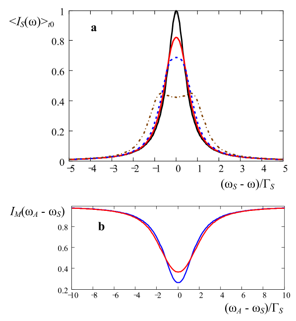
Figure 1: Power spectrum of the source radiation field, seen by the vibrated absorber, and absorption spectrum after passing through the absorber. a, Power spectrum, normalized to the peak intensity. b, The absorption spectrum, normalized to unity. The vibration frequency is $\Omega=\Gamma_{S}/5$. The modulation index $a$ is $0$ (solid black line), $2$ (solid red line), $3$ (blue dashed line), and 6 (brown dash-dotted line) in a. The modulation index $a$ is $0$ (blue line) and 6 (red line) in b. The optical thickness of the absorber is $T_{a}=\alpha(0)l=5.2$. The linewidth of the absorber $\Gamma_{A}$ and spectral components of the source $\Gamma_{S}$ are equal to $\Gamma_{0}$, which is defined by the lifetime of the excited state nucleus (141 ns).

Gamma-ray frequency combs were generated much earlier by Doppler modulation of the radiation frequency, induced by mechanical vibration of the source or resonant absorber Cranshaw ; Ruby ; Kornfeld ; Mishroy ; Walker ; Mkrtchyan77 ; Perlow ; Monahan ; Mkrtchyan79 ; Tsankov ; Shvydko89 ; Shvydko92 . They were observed in frequency domain and appear only if the source and absorber were used in couple. Contrary to the optical and X-ray combs, discussed above, gamma-ray frequency combs do not produce sharp, short pulses in time domain, except the cases if the specific conditions are satisfied Vagizov ; Shakhmuratov15 .

Gamma-ray frequency combs with high finesse $F\gg 1$, where $F$ is the ratio of the comb-tooth spacing to the tooth width, demonstrated that in many cases determination of small energy shifts between the source and absorber can be made more accurately in time domain by transient and high-frequency modulation techniques than by conventional methods in frequency domain Perlow ; Monahan ; Helisto1984 . We have to emphasize that in gamma domain even standard spectroscopic measurements with such a popular Mössbauer isotopes as ⁵⁷Fe and ⁶⁷Zn have already demonstrated extremely high frequency resolution in measurements of gravitational red-shift Pound1965 ; Potzel1992 . This is because the quality factor $Q$, which is the ratio of the resonance frequency to the linewidth, is very high for these nuclei. For example, 14.4 keV transition in ⁵⁷Fe has $Q=3\times 10^{12}$ and 93.3 keV resonance in ⁶⁷Zn demonstrates $Q=1.8\times 10^{15}$. Appropriate sources emitting resonant or very close to resonance $\gamma$-photons with high $Q$ are available for both nuclei. They are ⁵⁷Co for ⁵⁷Fe and ⁶⁷Ga for ⁶⁷Zn.

Here we show that a low finesse comb (LFC) with $F\ll 1$ is more sensitive to the small resonant detuning between the fundamental of the radiation field and the absorber compared with high finesse comb (HFC).

The basic idea of the modulation technique in gamma-domain is that the vibration of an absorber leads to a periodic modulation of the resonant nuclear transition frequency with respect to the frequency of the incident photons owing to the Doppler effect. This modulation induces coherent Raman scattering of the incident radiation in the forward direction transforming quasi-monochromatic field into a frequency comb at the exit of the absorber Shvydko92 . The relative amplitudes and phases of the produced spectral components are defined by the vibration amplitude $d$ and frequency $\Omega$, the detuning of the central frequency of the radiation source $\omega_{S}$ from the resonant frequency of the absorber $\omega_{A}$, the linewidths of the source $\Gamma_{S}$ and absorber $\Gamma_{A}$, and the absorber optical depth $T_{A}$. To describe the transformation of the quasi-monochromatic radiation field into a frequency comb it is convenient to consider the interaction of the field with nuclei in the reference frame rigidly bounded to the piston-like vibrated absorber. There, nuclei ‘see’ the quasi-monochromatic source radiation with main frequency $\omega_{S}$ as polychromatic radiation with a set of spectral lines $\omega_{S}\pm n\Omega$ ($n=0,\pm 1,\pm 2,...$) spaced apart at distances that are multiples of the oscillation frequency. The intensity of the $n$th sideband is given by the square of the Bessel function $J_{n}^{2}(a)$, here $a=2\pi d/\lambda$ is the modulation index of the field phase $\varphi(t)=a\sin(\Omega t)$, $d$ is the amplitude of the vibration, and $\lambda$ is the wavelength of the radiation.

If the modulation frequency $\Omega$ is much lager than $\Gamma_{S}$, the power spectrum of the radiation field, seen by the absorber nuclei, demonstrates HFC ($F=\Omega/\Gamma_{S}\gg 1$). It is observed in many Mössbauer experiments Cranshaw ; Ruby ; Kornfeld ; Mishroy ; Walker ; Mkrtchyan77 ; Perlow ; Monahan ; Mkrtchyan79 ; Tsankov ; Shvydko89 ; Shvydko92 by transmitting the radiation field through a single line absorber with resonant frequency $\omega_{A}$. The carrier frequency of the radiation frequency of the source $\omega_{S}$ is changed by a constant velocity Doppler shift. The intensity of the transmitted radiation, showing a frequency-comb Mössbauer spectrum, is described by equation

$$I_{M}(\omega_{A}-\omega_{S})={\displaystyle\int\limits_{-\infty}^{+\infty}}\left\langle I_{S}(\omega)\right\rangle_{t_{0}}e^{-\alpha(\omega_{A}-\omega)l}d\omega,$$ (1)

where $\alpha(\omega_{A}-\omega)$ is the frequency dependent absorption coefficient of the single line absorber, $l$ is the absorber thickness, and $\left\langle I_{S}(\omega)\right\rangle_{t_{0}}$ is the power spectrum of the radiation field seen by the vibrated nuclei. Here, the power spectrum is averaged over the random time of photon emission $t_{0}$ (see Supplementary information for details).

Frequency-domain Mössbauer spectrum is measured by counting the number of photons, detected within long time windows of the same duration for all resonant detunings, which are varied by changing the value of a constant velocity of the Mössbauer drive moving the source. Time windows are not synchronized with the mechanical vibration and their duration $T_{\text{w}}$ is much longer than the oscillation period $T_{\text{osc}}=2\pi/\Omega$.

If $F\ll 1$, the spectral components of the frequency comb, seen by the absorber nuclei, overlap resulting in the spectrum broadening of the radiation field (see Fig. 1a). Therefore Mössbauer spectra for LFC show only the line broadening with increase of the modulation index $a$, see Fig. 1b.

If time windows of the photon-count collection are synchronized with the phase oscillations and duration of the time-windows $T_{\text{w}}$ is much shorter than the oscillation period $T_{\text{osc}}$, then one can observe time dependence of the transmitted radiation. For HFC the number of counts $N(t)$, proportional to the radiation intensity $I(t)$, is described by the equation Perlow ; Monahan ; Helisto1984 ; Vagizov

$$N(t)=N_{0}{\displaystyle\sum_{n=0}^{\infty}}D_{n}\cos\left[n\Omega(t-t_{n})\right],$$ (2)

where $N_{0}$ is the number of counts without absorber, $D_{n}$ and $n\Omega t_{n}$ are the amplitude and phase of the $n$th harmonic. Here, nonresonant absorbtion is disregarded. Recoil processes in nuclear absorption and emission are not taken into account assuming that recoilless fraction (Debye-Waller factor) is $f=1$. These processes can be easily taken into account in experimental data analysis.

If the fundamental frequency $\omega_{S}$ of the comb coincides with the resonant frequency of the single line absorber ($\omega_{S}=\omega_{A}$), then the amplitudes of the odd harmonics are zero, $D_{2m+1}=0$, where $m$ is integer. They become nonzero for nonresonant excitation. For high finesse combs the ratio of the amplitudes of the first and second harmonics $D_{1}/D_{2}$ is linearly proportional to the resonant detuning $\Delta=\omega_{A}-\omega_{S}$ if the value of the modulation index $a$ is not large and the resonant detuning does not exceed the linewidth $(\Gamma_{A}+\Gamma_{S})/2$ Perlow ; Monahan . This dependence helps to measure the value of small resonant detuning with high accuracy Helisto1984 . For HFC the optimal value of the modulation index providing the best signal to noise ratio is $a=1.08$ when the amplitude of the first harmonic $D_{1}$ takes maximum. This is because for HFC $D_{1}$ is proportional to the product of the amplitudes of zero and first components of the comb, i.e., to $J_{0}(a)J_{1}(a)$.

If one of the sidebands of the comb ($\omega_{S}\pm n\Omega$) is in resonance with the absorber ($\omega_{S}\pm n\Omega=\omega_{A}$, $n\neq 0$), then time dependence of the radiation field shows large amplitude pulses of short duration Vagizov ; Shakhmuratov15 . High sensitivity of HFC to resonance of its central frequency with a single line absorber and formation of short pulses if the sidebands are in resonance are explained by the interference of the spectral components of the comb, which are changed after passing through the absorber. In this paper we show that LFC is much more sensitive to the resonance of the central component of the comb with the single line absorber. This sensitivity can be explained by the following arguments.

Since the radiation intensity is $I(t)=E(t)E^{\ast}(t)$, which is the product of the complex conjugated amplitudes $E(t)$ containing the exponential phase factor $\exp[i\varphi(t)]$, the time dependent phase $\varphi(t)$ of the field amplitude does not lead to the additional time dependence of the intensity. This fact, resulting from the simple relation $e^{i\varphi(t)}e^{-i\varphi(t)}=1$, can be explained by a particular interference of the spectral components of this specific frequency comb. For example, only zero frequency spectral component is present in the intensity, $I(t)=\mathtt{I}_{0}$, since all zero spectral components, resulting from the products $e^{in\Omega t}e^{-in\Omega t}$ with $n=0,\pm 1,\pm 2...$, are summed up with the equal weights as

$${\displaystyle\sum\limits_{n=-\infty}^{+\infty}}J_{n}^{2}(a)=1,$$ (3)

while the first harmonic $I_{1}(t)e^{i\Omega t}$ is zero because this sum gives

$${\displaystyle\sum\limits_{n=-\infty}^{+\infty}}J_{n}(a)J_{n-1}(a)=0.$$ (4)

The same is true for all higher frequency components. This fragile balance between spectral components is easily broken after passing through the single line absorber. We found that for LFC the absorber of thickness $l$ satisfying the relation $\alpha(0)l=1$ is already capable to produce noticeable time oscillations of the intensity. These oscillations are also described by Eq. (2) whose coefficients can be calculated by the method developed in Monahan ; Vagizov (see details in Supplementary information). In contrast to HFC ($\Omega\gg\Gamma_{S}$), LFC ($\Omega\ll\Gamma_{S}$) becomes sensitive to exact resonance if effective halfwidth of the comb $a\Omega$ is nearly equal to the width of the absorption line $\Gamma_{A}$. Since for LFS $a\gg 1$, much more spectral components [$J_{n}(a)J_{n+1}(a)$ with $n=0,\pm 1,...,\pm a$] participate in the interference compared with HFC. Thus, the spectral content of the intensity oscillations becomes more sensitive to the resonant detuning.

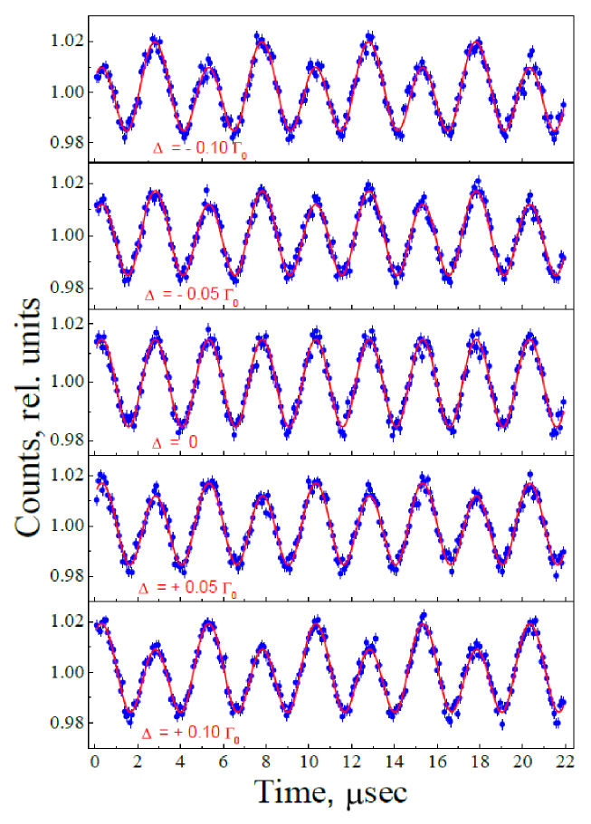
Figure 2: Time dependence of the photon counts $N(t)$ for different values of the resonant detuning. The number of counts (in relative units) are normalized to the mean value at exact resonance. The value of the detuning in units of $\Gamma_{0}$ is indicated in each panel. The dots are experimental points and solid line is a theoretical fitting.

.

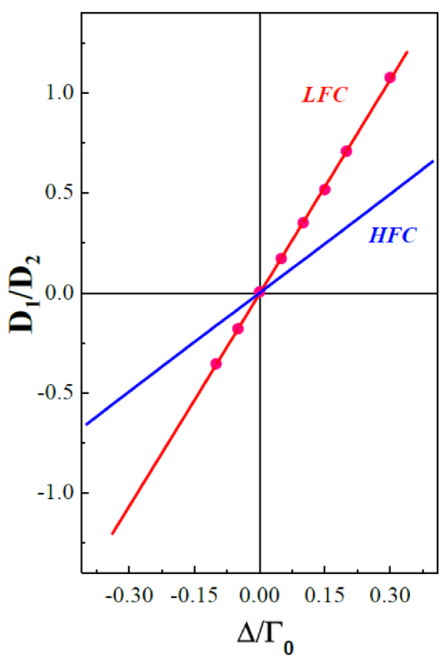
Figure 3: Dependence of the ratio of the amplitudes of the first and second harmonics of the intensity oscillations on resonant detuning. Comparison of the dependence of $D_{1}/D_{2}$ on $\Delta$ for LFC and HFC. Experimental data for LFC are shown by dots.

.

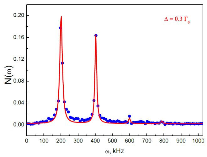
Figure 4: Fourier content of the oscillations. Fourier content of the intensity oscillations for $\Delta=0.3\Gamma_{S}$. Other parameters are defined in the text. Dots correspond to the data, obtained from the Fourier analysis of the experimentally observed intensity oscillations. Solid line is the analytical approximation by the set of Lorentzians.

We demonstrated LFC sensitivity in the experiments with the radiation source, which is a radioactive ⁵⁷Co incorporated into rhodium matrix. The source emits 14.4 keV photons with the spectral width $\Gamma_{S}=1.13$ MHz, which is mainly defined by the lifetime of 14.4 keV excited state of ⁵⁷Fe, the intermediate state in the cascade decay of ⁵⁷Co to the ground state ⁵⁷Fe. The absorber is a 25-$\mu$m-thick stainless-steel foil with a natural abundance ($\sim$ 2%) of ⁵⁷Fe. Optical depth of the absorber is $T_{A}=\alpha(0)l=5.18$. The stainless-steel foil is glued on the polyvinylidene fluoride piezo-transducer that transforms the sinusoidal signal from radio-frequency generator into the uniform vibration of the foil. The frequency and amplitude of the sinusoidal voltage were adjusted to have $\Omega=200$ kHz and $a=5.7$, so that relation $a\Omega\approx\Gamma_{A}$ was satisfied. The source is attached to the holder of the Mössbauer transducer causing Doppler shift of the radiation field to tune the source in resonance or out of resonance with the single line absorber. The time measurements were performed by means of the time–amplitude converter (TAC) working in the start–stop mode. The start pulses for the converter were synchronized with radio-frequency generator and the stop pulses were formed from the signal of 14.4 keV gamma counter at the instant of photon detection time. A detailed description of the experimental setup is given in Vagizov ; Shakhmuratov15 .

The experimental results demonstrating the oscillations of the radiation intensity in time for different values of the resonant detunings $\Delta$ are shown in Fig. 2. Time dependence of the number of counts is fitted to Eq. (2) (see details in Supplementary information). At exact resonance ($\Delta=0$) only even harmonics are not zero. Time delay of the second harmonic with respect to the vibration phase is $t_{2}=61$ ns. This delay is caused by the contribution of dispersion, which produces a phase shift $2\Omega t_{2}$. The Fourier analysis of the oscillations allows to reconstruct the dependence of the ratio $D_{1}/D_{2}$ on $\Delta$, which is shown in Fig. 3. This dependence is compared with that for HFC, generated by the vibration with high frequency $\Omega=10$ MHz and optimal value of the modulation index $a=1.08$. We see that LFC is at least two times more sensitive to resonance than HFC since the slope of the dependence of $D_{1}/D_{2}$ on $\Delta$ is two times steeper.

Figure 4 shows the Fourier content of the oscillations of the radiation intensity for LFC when $\Delta=0.3\Gamma_{S}$. The spectrum of these oscillations contains noticable contributions of the first, second, and third harmonics. The width of these spectral components is defined by the length of the time window where the oscillations are measured. In our experiments the spectral width of each Fourier component is close to 10 kHz. Thus, we may conclude that within a moderate time of experiment the proposed method is able to measure the resonant detuning for ⁵⁷Fe with the accuracy of 10 kilohertz, which is 100 times smaller than the absorption linewidth. This is essentially better accuracy than in the method of the resonant detuning measurements, used in the gravitational red-shift measurements Pound1965 ; Cranshaw , which employs four known values of the calibrated, controllable resonant detunings: two very large, comparable with the absorption halfwidth, and two very small, comparable but appreciably exceeding the measured detuning. In time domain measurements, by extending considerably the length of the time window where the oscillations are collected, one can reach even higher accuracy of several Hz.

Concluding, we demonstrate a method how with LFC one can measure precisely the resonant frequency of the absorber with the accuracy equal to a tiny fraction of the homogeneous absorption width. This method is also applicable in optical domain. Modulation of the resonant frequency of atoms or impurity ions by Stark/Zeeman effects or modulation of the frequency of the laser beam by acousto-optical modulator are equivalent to creation of a frequency comb in a particular reference frame. The interference of the scattered radiation field with the incident field is capable to produce the output intensity oscillations. By a proper choice of the modulation frequency and modulation index one can make this oscillations to be very sensitive to exact resonance or to measure the frequency difference between the incident radiation and resonance frequency of atoms with the accuracy not limited by the value of the homogeneous linewidth.

I METHODS SUMMARY

The transformation of a spontaneously emitted gamma-radiation on its propagation through a uniformly vibrating, resonant Mössbauer absorber is described semiclassically in the linear response approximation. Time dependence of the radiation intensity at the exit of the absorber is studied as a function of the parameters of the system, such as the frequency and amplitude of modulation, the detuning of the central frequency of the source from the resonance frequency of the absorber. We numerically plot the intensity for different parameter values to demonstrate how the oscillations depend on the resonant detuning. Optimal values of the modulation index are found for the observation of noticeable effect.

Acknowledgements This work was partially funded by the Russian Foundation for Basic Research (Grant No. 15-02-09039-a), the Program of Competitive Growth of Kazan Federal University funded by the Russian Government, the RAS Presidium Programs “Fundamental optical spectroscopy and its applications”and “Actual problems of low temperature physics”, the National Science Foundation (Grant No. PHY-1307346), and the Robert A. Welch Foundation (Award A-1261).

II Supplementary Information

In this Supplementary information we give details of mathematical description of the gamma-radiation intensity oscillations in time for high and low finesse frequency combs.

II.1 Introductory remarks

The propagation of gamma radiation through a resonant Mössbauer medium vibrating with frequency $\Omega$ may be treated classically Ikonen1985* (the references are given at the end of the section in the separate list). In this approach the radiation field from the source nucleus after passing through a small diaphragm is approximated as a plane wave propagating along the direction $\mathbf{x}$. In the coordinate system rigidly bounded to the absorbing sample, the field, seen by the absorber nuclei, is described by

$$E_{S}(t-t_{0})\propto\theta(t-t_{0})e^{-(i\omega_{S}+\Gamma_{0}/2)(t-t_{0})+ikx+i\varphi(t)},$$ (5)

where $\omega_{S}$ and $k$ are the carrier frequency and the wave number of the radiation field, $1/\Gamma_{0}$ is the lifetime of the excited state of the emitting source nucleus, $t_{0}$ is the instant of time when the excited state is formed, $\Theta(t-t_{0})$ is the Heaviside step-function, $\varphi(t)=2\pi x_{d}(t)/\lambda=a\sin(\Omega t)$ is a time dependent phase of the field due to a piston-like periodical displacement of the absorber with respect to the source, $x_{d}(t)$, and $\lambda$ is the radiation wavelength.

It can be easily shown that radiation intensity at the exit of the vibrating absorber is the same if the source is vibrated instead of absorber. For simplicity we consider the vibration of the source with respect to the absorber and not vice versa, since both cases are equivalent. Then the radiation field from the source can be expressed as follows

$$E_{S}(t-t_{0})=E_{C}(t-t_{0})e^{-i\omega_{S}(t-t_{0})+ikx}\sum_{n=-\infty}^{+\infty}J_{n}(a)e^{in\Omega t},$$ (6)

where $E_{C}(t-t_{0})=E_{0}\theta(t-t_{0})e^{-\Gamma_{0}(t-t_{0})/2}$ is the common part of the field components, $E_{0}$ is the field amplitude, and $J_{n}(a)$ is the Bessel function of the $n$th order. The Fourier transform of this field is

$$E_{S}(\omega)=E_{0}\sum_{n=-\infty}^{+\infty}\frac{J_{n}(a)e^{in\Omega t_{0}}}{\Gamma_{0}/2+i(\omega_{S}-n\Omega-\omega)},$$ (7)

where for shortening of notations the exponential factor with $ikx$ is omitted. From this expression, it is clear that the vibrating absorber ‘sees’ the incident radiation as an equidistant frequency comb with spectral components $\omega_{S}-n\Omega$ whose amplitudes are proportional to $J_{n}(a)$. Below, for briefness we use the shortened notation $J_{n}(a)=J_{n}$.

According to Eq. (5) the intensity of the field

$$I(t-t_{0})=\left|E_{S}(t-t_{0})\right|^{2}=I_{0}\theta(t-t_{0})e^{-\Gamma_{0}(t-t_{0})},$$ (8)

where $I_{0}=E_{0}^{2}$, does not oscillate in time. The same result must be obtained from Eq. (6), which gives

$$\left|E_{S}(t-t_{0})\right|^{2}=\left|E_{C}(t-t_{0})\right|^{2}\sum_{n=-\infty}^{+\infty}\sum_{m=-\infty}^{+\infty}J_{n}J_{m}e^{i(n-m)\Omega t},$$ (9)

where $\left|E_{C}(t-t_{0})\right|^{2}=I_{0}(t-t_{0})$ according to the definition. Therefore, the identity

$$\sum_{n=-\infty}^{+\infty}\sum_{m=-\infty}^{+\infty}J_{n}J_{m}e^{i(n-m)\Omega t}=1$$ (10)

is to be satisfied. It is consistent with the well known relations between the Bessel functions (see, for example, AbramSteg65* ). They are

$$\sum_{n=-\infty}^{+\infty}J_{n}^{2}=J_{0}^{2}+2\sum_{n=1}^{+\infty}J_{n}^{2}=1$$ (11)

for zero harmonic ($n=m$), which is the only harmonic giving nonzero contribution into the radiation intensity in Eq. (9) due to Eq. (10), and

$$\sum_{n=-\infty}^{+\infty}J_{n}J_{n+2}=-J_{1}^{2}+2\sum_{n=0}^{+\infty}J_{n}J_{n+2}=0,$$ (12)

for the second harmonic ($-2\Omega$) with $m=n+2$ in Eq. (9), and

$$\sum_{n=-\infty}^{+\infty}J_{n}J_{n+4}=J_{2}^{2}-2J_{1}J_{3}+2\sum_{n=0}^{+\infty}J_{n}J_{n+4}=0,$$ (13)

for the fourth harmonic ($-4\Omega$) with $m=n+4$. It can be easily shown that all even harmonics do not contribute since their amplitudes are zero. As regards the odd harmonics, they have zero amplitudes because of the cancelation of the symmetric pairs in their content as, for example, for the first harmonic ($-\Omega$) with $m=n+1$,

$$\sum_{n=-\infty}^{+\infty}J_{n}J_{n+1}=(J_{0}J_{1}+J_{-1}J_{0})+(J_{1}J_{2}+J_{-2}J_{-1})+...=0,$$ (14)

and the third harmonic ($-3\Omega$) with $m=n+3$,

$$\sum_{n=-\infty}^{+\infty}J_{n}J_{n+3}=(J_{0}J_{3}+J_{-3}J_{0})+(J_{1}J_{4}+J_{-4}J_{-1})+...=0.$$ (15)

Here the property of the Bessel function, $J_{-n}=(-1)^{n}J_{n}$ (where $n$ is positive), is taken into account.

If such a field with balanced amplitudes and phases of its harmonics, Eq. (6), passes through a thick resonant absorber, one may expect that this balance will be broken and the intensity of the field at the exit of the absorber will be oscillating.

II.2 The transformation of the radiation field after passing through a resonant absorber

The Fourier transform of the radiation field is changed at the exit of the resonant absorber as Monahan* ; Vagizov*

$$E_{out}(\omega)=E_{0}\sum_{n=-\infty}^{+\infty}\frac{J_{n}\exp\left[in\Omega t_{0}-\frac{b}{\Gamma_{A}/2+i(\omega_{A}-\omega)}\right]}{\Gamma_{0}/2+i(\omega_{S}-n\Omega-\omega)},$$ (16)

where $\omega_{A}$ and $\Gamma_{A}$ are the frequency and linewidth of the absorber, $b=T_{A}\Gamma_{0}/4$ is the parameter depending on the effective thickness of the absorber $T_{A}=fn\sigma$, $f$ is the Debye-Waller factor, $n$ is the number of ⁵⁷Fe nuclei per unit area of the absorber, and $\sigma$ is the resonance absorption cross section. The source linewidth $\Gamma_{S}$ can be different from $\Gamma_{0}$ due to the contribution of the environment of the emitting nucleus in the source. In this case $\Gamma_{0}$ can be simply substituted by $\Gamma_{S}$ in Eq. (16).

Time dependence of the amplitude of the output radiation field is found by inverse Fourier transformation

$$E_{out}(t-t_{0})=\frac{1}{2\pi}\int_{-\infty}^{+\infty}E_{out}(\omega)e^{-i\omega(t-t_{0})}d\omega.$$ (17)

Then, the intensity of the field is

$$I_{out}(t-t_{0})=\frac{1}{(2\pi)^{2}}\int_{-\infty}^{+\infty}d\omega_{1}\int_{-\infty}^{+\infty}d\omega_{2}E_{out}(\omega_{1})E_{out}^{\ast}(\omega_{2})e^{i(\omega_{2}-\omega_{1})(t-t_{0})}.$$ (18)

In time domain experiments the phase of the vibrations is fixed but emission time of gamma-photons is random. Therefore, the observed radiation intensity is averaged over $t_{0}$

$$\left\langle I_{out}(t-t_{0})\right\rangle_{t_{0}}=\lim_{T\rightarrow\infty}\int_{-T}^{t}I_{out}(t-t_{0})dt_{0}.$$ (19)

Calculation of this integral gives for the number of gamma-photon counts at the exit of the absorber, $N_{out}(t)\propto\left\langle I_{out}(t-t_{0})\right\rangle_{t_{0}}$, the following expression Vagizov*

$$N_{out}(t)/N_{0}=\sum_{n,m=-\infty}^{+\infty}J_{n}J_{m}e^{i(n-m)\Omega t}B_{nm}(\Delta),$$ (20)

where $N_{0}$ is the number of counts far from resonance and

$$B_{nm}(\Delta)=\frac{\Gamma_{S}}{2\pi}\int_{-\infty}^{+\infty}\frac{e^{-\frac{b}{\Gamma_{A}/2+i(\Delta+n\Omega-\omega)}-\frac{b}{\Gamma_{A}/2-i(\Delta+m\Omega-\omega)}}}{(\Gamma_{S}/2)^{2}+\omega^{2}}d\omega,$$ (21)

where $\Delta=\omega_{A}-\omega_{S}$ is the resonance detuning of the source and absorber. In derivation of Eq. (21) the substitution $\omega^{\prime}=\omega-\omega_{S}+n\Omega$ is used in Eqs. (16) and (18). Then the prime is omitted.

II.3 Intensity oscillations

To analyze the oscillations of the radiation intensity after passing through the vibrated absorber it is convenient to group the terms in Eq. (20) as follows

$$N_{out}(t)/N_{0}=\mathtt{I}_{0}(\Delta)+2\operatorname{Re}\sum_{n=1}^{+\infty}\mathtt{I}_{n}(\Delta)e^{-in\Omega t},$$ (22)

where $\mathtt{I}_{n}(\Delta)$ is the $n$th-harmonic amplitude of the radiation intensity oscillations at the exit of the absorber. The amplitudes of the harmonics are defined by the products of the radiation amplitudes of the frequency comb (16), transformed by the absorber. For example, the amplitude of zero harmonic is

$$\mathtt{I}_{0}(\Delta)=J_{0}^{2}B_{00}(\Delta)+\sum_{n=1}^{+\infty}J_{n}^{2}\left[B_{nn}(\Delta)+B_{(-n)(-n)}(\Delta)\right],$$ (23)

where the coefficients $B_{00}(\Delta)$, $B_{nn}(\Delta)$, and $B_{(-n)(-n)}(\Delta)$ are transmitted intensities of $0$, $n$, and $-n$ components of the incident comb (6). They are

$$B_{00}(\Delta)=\frac{\Gamma_{S}}{2\pi}\int_{-\infty}^{+\infty}\frac{e^{-\frac{b\Gamma_{A}}{(\Gamma_{A}/2)^{2}+(\Delta-\omega)^{2}}}}{(\Gamma_{S}/2)^{2}+\omega^{2}}d\omega,$$ (24)

$$B_{(\pm n)(\pm n)}(\Delta)=\frac{\Gamma_{S}}{2\pi}\int_{-\infty}^{+\infty}\frac{e^{-\frac{b\Gamma_{A}}{(\Gamma_{A}/2)^{2}+(\Delta\pm n\Omega-\omega)^{2}}}}{(\Gamma_{S}/2)^{2}+\omega^{2}}d\omega.$$ (25)

Thus, $\mathtt{I}_{0}(\Delta)$ is just the sum of the transmitted intensities of all spectral components of the frequency comb (6).

The first harmonic

$$\mathtt{I}_{1}(\Delta)=\sum_{n=0}^{+\infty}J_{n}J_{n+1}\left[B_{n(n+1)}(\Delta)-B_{(-n-1)(-n)}(\Delta)\right],$$ (26)

contains the difference of two terms originating from the interference of two neighboring components of the frequency comb $\pm n$ and $\pm(n+1)$. They are red (for sign $+$) and blue (for sign $-$) detuned from resonance. This difference is

$$B_{n(n+1)}(\Delta)-B_{(-n-1)(-n)}(\Delta)=\\ \frac{\Gamma_{S}}{2\pi}\int_{-\infty}^{+\infty}\frac{e^{-\frac{b}{\Gamma_{A}/2+i(\Delta+n\Omega-\omega)}-\frac{b}{\Gamma_{A}/2-i[\Delta+(n+1)\Omega-\omega]}}-e^{-\frac{b}{\Gamma_{A}/2+i[\Delta-(n+1)\Omega-\omega]}-\frac{b}{\Gamma_{A}/2-i(\Delta-n\Omega-\omega)}}}{(\Gamma_{S}/2)^{2}+\omega^{2}}d\omega.$$ (27)

It is easy to show (by substitution $\omega=-\omega^{\prime}$ in the second exponent) that the difference of the interference terms is zero if $\Delta=0$.

The second and third harmonics are described by equations

$$\mathtt{I}_{2}(\Delta)=-J_{1}^{2}B_{-11}(\Delta)+\sum_{n=0}^{+\infty}J_{n}J_{n+2}\left[B_{n(n+2)}(\Delta)+B_{(-n-2)(-n)}(\Delta)\right],$$ (28)

$$\mathtt{I}_{3}(\Delta)=-J_{1}J_{2}[B_{-12}(\Delta)-B_{-21}(\Delta)]+\sum_{n=0}^{+\infty}J_{n}J_{n+3}\left[B_{n(n+3)}(\Delta)-B_{(-n-3)(-n)}(\Delta)\right],$$ (29)

which contain the interference terms of the frequency-comb amplitudes with $m-n=2$ for $\mathtt{I}_{2}(\Delta)$ and $m-n=3$ for $\mathtt{I}_{3}(\Delta)$ [see Eq. (21)]. The third harmonic is zero if $\Delta=0$ because it contains the difference of the interference terms, while the second harmonic is not zero since it is the sum of the interference terms.

The coefficients $D_{n}$ in equation (2) of the main part of the manuscript, describing the number of count oscillations in time, are related to the harmonics $\mathtt{I}_{n}(\Delta)$ as $D_{0}=\mathtt{I}_{0}(\Delta)$, $D_{2n}=2\left|\mathtt{I}_{2n}(\Delta)\right|$, and $D_{2n+1}=2S(\Delta)\left|\mathtt{I}_{2n+1}(\Delta)\right|$, where $S(\Delta)=\Delta/\left|\Delta\right|$. The phases of the harmonics are defined as $\Omega t_{n}=\arctan\left[\operatorname{Im}\mathtt{I}_{n}(\Delta)/\operatorname{Re}\mathtt{I}_{n}(\Delta)\right]$.

II.4 High finesse frequency comb

If the modulation frequency is much larger than the absorption linewidth ($\Omega\gg\Gamma_{A}$) and the central frequency of the comb $\omega_{S}$ is close to the resonant frequency of the absorber $\omega_{A}$ ($\left|\Delta\right|<\Gamma_{A}$), then only the central frequency of the comb is changed after passing through a thick absorber. Therefore, one may expect that in Eq. (20) only the components $B_{00}$, $B_{0n}$ and $B_{n0}$ become different from $1$, while others are almost unity since for them the exponents in the integral (21) are unity if the condition $n\Omega\gg b$ is satisfied. In this case we can use approximate equations

$$\mathtt{I}_{0}(\Delta)\approx 1-J_{0}^{2}[1-B_{00}(\Delta)],$$ (30)

$$\mathtt{I}_{1}(\Delta)\approx J_{0}J_{1}\left[B_{01}(\Delta)-B_{-10}(\Delta)\right],$$ (31)

$$\mathtt{I}_{2}(\Delta)\approx J_{0}J_{2}\left[B_{02}(\Delta)+B_{-20}(\Delta)-2\right],$$ (32)

which are derived taking into account the relations (11), (12), and (14). The product $J_{0}J_{1}=J_{0}(a)J_{1}(a)$ in Eq. (31) has global maximum when the modulation index is $a=1.08$. Therefore, for nonresonant excitation ($\Delta\neq 0$ and $\left|\Delta\right|<\Gamma_{A}$) the first harmonic of the intensity oscillations has maximum amplitude for this value of the modulation index. Since it is not large, we may approximate the intensity oscillations taking into account only three harmonics $n=0,1,2$ in Eq. (22).

Figure 5: Oscillations of the radiation intensity for high finesse comb ($\Omega$=10 MHz) are shown by solid lines. The resonant detuning is $\Delta=-200$ kHz in (a) and $\Delta=200$ kHz in (b). Dotted line shows the level of $\mathtt{I}_{0}(\Delta)$. The value of the parameters are given in the text.

However, to achieve high accuracy we have to take into account also the contribution of two spectral components of the comb, neighboring the resonant component Shakhmuratov15* . This is because far wings of the Lorentzian line give small, but noticable contribution. In our case, when the central component of the comb is in resonance, these nearest components are $+\Omega$ and $-\Omega$. Then, for example, $\mathtt{I}_{0}(\Delta)$ is modified due to this small nonresonant contribution as

$$\mathtt{I}_{0}(\Delta)=1-J_{0}^{2}[1-B_{00}(\Delta)]-J_{1}^{2}[2-B_{11}(\Delta)-B_{-1-1}(\Delta)].$$ (33)

The value of the correction due to the additional terms is about 2% if $\Omega/\Gamma_{0}=10$, $\Delta=0.2\Gamma_{0}$, and $T_{A}=5$.

In conclusion of this section, we show in Fig. 5 two examples of the intensity oscillations (not approximated) for $\Gamma_{A}=\Gamma_{S}=\Gamma_{0}=1.13$ MHz, $T_{A}=5.2$, $\Omega=10$ MHz, $a=1.08$, and $\Delta=\pm 200$ kHz. The dependence of $D_{1}/D_{2}$ on $\Delta$ (not approximated) is shown in Fig. 3 of the main part of the manuscript.

II.5 Low finesse comb

For the low finesse comb the modulation frequency is much smaller than the absorption linewidth ($\Omega\ll\Gamma_{A}$). If the central frequency of the comb $\omega_{S}$ is close to the resonant frequency of the absorber $\omega_{A}$ ($\left|\Delta\right|<\Gamma_{A}$), then many spectral components of the comb are changed after passing through a thick absorber. Therefore, to describe the oscillation of the output radiation intensity we have to take many terms in the equations (23), (26), (28), and (29) for $\mathtt{I}_{n}(\Delta)$, $n=0,1,2,3$.

Intuitively, one may expect that LFC sensitivity is maximal if all noticeable components of the comb are modified after passing through the absorber. This takes place if the product $a\Omega$, which specifies the total spectral width of the comb or the frequency range, covered by the comb components with noticeable amplitudes, is close to the width of the absorption line. Mathematically, this expectation can be verified by plotting the amplitude $D_{1}=2S(\Delta)\left|\mathtt{I}_{1}(\Delta)\right|$ versus modulation index $a$ for a fixed values of the modulation frequency $\Omega$ and resonant detuning $\Delta$. Figure 6 shows the dependence of $D_{1}$ on the modulation index $a$ for $\Omega=\Delta=200$ kHz and $T_{A}=5.2$. The amplitude $D_{1}$ takes maximum value when $a=7$. For this value the product $a\Omega$ is close to the linewidth of the absorber $\Gamma_{A}$.

Figure 6: The dependence of the first-harmonic amplitude $D_{1}$ of the intensity oscillations on the modulation index $a$. The modulation frequency and resonant detuning are $\Omega=\Delta=200$ kHz.

References

- (1) Udem, Th., Holzwarth, R. & Hänsch, T. W. Optical frequency metrology. Nature 416, 233-237 (2002).
- (2) Cundiff, S. T. & Ye, J. Colloquium: Femtosecond optical frequency combs. Rev. Mod. Phys. 75, 325-342 (2003).
- (3) Bartels, A., Oates, C. W., Hollberg, L. & Diddams, S. A. Stabilization of femtosecond laser frequency combs with subhertz residual linewidths. Optics Letters 29, 1081-1083 (2004).
- (4) Schibli, T. R., Hartl, I., Yost, D. C., Martin, M., J., Marcinkevičius, A., Fermann, M. E. & Ye, J. Optical frequency comb with submillihertz linewidth and more than 10 W average power. Nature Photonics 2, 355 - 359 (2008).
- (5) Fang, S., Chen, H., Wang, T., Jiang, Y., Bi, Z. & Ma, L. Optical frequency comb with an absolute linewidth of 0.6 Hz - 1.2 Hz over an octave spectrum. Appl. Phys. Lett. 102, 231118 (2013).
- (6) Udem, Th., Reichert, J., Holzwarth, R. & Hänsch, T. W. Absolute optical frequency measurement of the cesium line with a mode-locked laser. Phys. Rev. Lett. 82, 3568–3571 (1999).
- (7) Jones, D. J., Diddams, S. A., Ranka, J. K., Stentz A., Windeler, R. S., Hall, J. L., & Cundiff, S. T. Carrier-envelope phase control of femtosecond mode-locked lasers and direct optical frequency synthesis. Science 288, 635–639 (2000).
- (8) Niering, M., Holzwarth, R., Reichert, J., Pokasov, P., Udem, Th., Weitz, M & Hänsch, T. W. Measurement of the hydrogen 1S-2S transition frequency by phase coherent comparison with a microwave cesium fountain clock. Phys. Rev. Lett. 84, 5496–5499 (2000).
- (9) Diddams, S. A., Jones, D. J., Ye, J., Cundiff, S. T., Hall, J. L., Ranka, J. K., Windeler, R. S., Holzwarth, R., Udem, Th. & Hänsch, T. W. Direct link between microwave and optical frequencies with a 300 THz femtosecond laser comb. Phys. Rev. Lett. 84, 5496–5499 (2000).
- (10) Udem, Th., Diddams, S. A., Vogel, K. R., Oates, C. W., Curtis, E. A., Lee, W. D., Itano, W. M., Drullinger, R. E., Bergquist, J. C., Hollberg, L. Absolute frequency measurements of the Hg+ and Ca optical clock transitions with a femtosecond laser. Phys. Rev. Lett. 86, 4996–4999 (2001).
- (11) Diddams, S. A., Udem, Th., Bergquist, J. C., Curtis, E. A., Drullinger, R. E., Hollberg, L., Itano, W. M., Lee, W. D., Oates, C. W., Vogel, K. R. & Wineland D. J. An optical clock based on a single trapped 199Hg. Science 293, 825-828 (2001).
- (12) Ye, J., Ma, L. S. & Hall, J. L. Molecular iodine clock. Phys. Rev. Lett. 87, 270801 (2001).
- (13) Stowe, M. C., Cruz, F. C., Marian, A. & Ye, J. High resolution atomic coherent control via spectral phase manipulation of an optical frequency comb. Phys. Rev. Lett. 96, 153001 (2006).
- (14) Steinmetz, T., Wilken, T, Araujo-Hauck, C., Holzwarth, R., Hänsch, T. W., Pasquini, L, Manescau, A., D’Odorico, S., Murphy, M. T., Kentischer, T., Schmidt, W. & Udem, Th. Laser frequency combs for astronomical observations. Science 321, 1335–1337 (2008).
- (15) Cavaletto, S. M., Harman, Z., Ott, C., Buth, C., Pfeifer, T. & Keitel, C. H. Broadband high-resolution X-ray frequency combs. Nature Photonics 8, 520-523 (2014).
- (16) Liu, Z., Cavaletto, S. M., Harman, Z., Keitel, C. H. & Pfeifer, T. Generation of high-frequency combs locked to atomic resoannces by quantum phase modulation. New Journal of Physics 16, 093005 (2014).
- (17) Cranshaw, T. E. & Reivari, P. A Mössbauer study of the hyperfine spectrum of 57Fe, using ultrasonic calibration. Proc. Phys. Soc. 90, 1059-1064 (1967).
- (18) Ruby, S. L. & Bolef, D. I. Acoustically modulated rays from Fe57. Phys. Rev. 5, 5-7 (1960).
- (19) Kornfeld, G. Line shape of the Mössbauer line in the presence of ultrasonic vibrations with decaying amplitudes. Phys. Rev. 177, 494-501 (1969).
- (20) Mishroy, J. & Bolef, D. I. Interaction of ultrasound with Mössbauer gamma rays. Mössbauer Effect Methodology, edited by I. J. Gruverman (Plenum Press, Inc. Ney York, 1968), Vol. 4, P. 13-35.
- (21) Chein, C. L. & Walker, J. C. Mössbauer sidebands from a single parent line. Phys. Rev. B 13, 1876-1879 (1976).
- (22) Mkrtchyan, A. R., Arakelyan, A. F., Arutyunyan, G. A. & Kocharyan, L. A. Oscillations of the Mössbauer spectrum line intensity following modulation by coherent ultrasound. JETP Lett. 26, 449-452 (1977).
- (23) Perlow, G. J. Quantum beats of recoil-free radiation. Phys. Rev. Lett. 40, 896-899 (1978).
- (24) Monahan, J. E. & Perlow, G. J. Theoretical description of quantum beats of recoil-free radiation. Phys. Rev. A 20, 1499-1510 (1979).
- (25) Mkrtchyan, A. R. Arutyunyan, G. A. Arakelyan, A. R. & Gabrielyan, R. G. Modulation of Mössbauer radiation by coherent ultrasonic excitation in crystals Phys. Stat. Sol B 92, 23-29 (1979).
- (26) Tsankov, L. T. Experimental observation on the resonant amplitude modulation of Mössbauer gamma rays. J. Phys. A: Math. Gen. 14, 275-281 (1981).
- (27) Popov, S. L. Smirnov, G. V. & Svyd’ko, Yu. V. Observed strengthening of radioactive mechanism for a nuclear reaction in the interaction of radiation with nuclei in a vibrating absorber. JETP Lett. 49, 747-751 (1989).
- (28) Svyd’ko, Yu. V. & Smirnov, G. V. Enhanced yield into the radiative channel in Raman nuclear resonant forward scattering. J. Phys.: Condens. Matter 4, 2663-2685 (1992).
- (29) Vagizov, F., Antonov, V., Radeonychev, Y. V., Shakhmuratov, R. N. & Kocharovskaya, O. Coherent control of the waveforms of recoilless -ray photons. Nature 508, 80-83 (2014).
- (30) Shakhmuratov, R. N., Vagizov, F. G., Antonov, V. A., Radeonychev, Y. V., Scully, M. O. & Kocharovskaya, O. Transformation of a single-photon field into bunches of pulses. Phys. Rev. A 92, 023836 (2015).
- (31) Helistö, P., Ikonen, E., Katila, T., Potzel, W. & Riski, K. Precision determination of small energy shifts in Mössbauer spectroscopy. Phys. Rev. B 30, 2345-2352 (1984).
- (32) Pound, R. V. & Snider, J. L. Effect of gravity on gamma radiation. Phys. Rev. 140, B788-B803 (1965).
- (33) Potzel, W., Schäfer, C., Steiner, M., Karzel, H., Schiessl, W., Peter, M., Kalvius, G. M., Katila, T., Ikonen., E., Helistö & Hietaniemi, J. Gravitational redshift experiments with the high-resolution Mössbauer resonance in 67Zn. Hyperfine Interactions 72, 197-214 (1992).

References

- (1) Ikonen, E., Helistö, P., Katila, T. & Riski, K. Coherent transient effects due to phase modulation of recoilless radiation. Phys. Rev. A 32, 2298 (1985).
- (2) Handbook of Mathematical Functions, edited by M. Abramowitz and I. A. Stegun (Dover, New York, 1965).
- (3) Monahan, J. E. & Perlow, G. J. Theoretical description of quantum beats of recoil-free radiation. Phys. Rev. A 20, 1499-1510 (1979).
- (4) Vagizov, F., Antonov, V., Radeonychev, Y. V., Shakhmuratov, R. N. & Kocharovskaya, O. Coherent control of the waveforms of recoilless -ray photons. Nature 508, 80-83 (2014).
- (5) Shakhmuratov, R. N., Vagizov, F. G., Antonov, V. A., Radeonychev, Y. V., Scully, M. O. & Kocharovskaya, O. Transformation of a single photon field into bunches of pulses. Phys. Rev. A 92, 023836 (2015).