Water in Asbestos

Abstract

We present the molecular simulation study of the behavior of water and sodium chloride solution confined in lizardite asbestos nanotube which is a typical example of hydrophilic confinement. The local structure, orientational and dynamic properties are studied. It is shown that the diffusion coefficient drops about two orders of magnitude comparing to the bulk case, and water in lizardite asbestos tubes experiences vitrification rather then crystallization upon cooling in accordance with the results for some other hydrophilic confinements. The behavior of sodium chloride solutions also considered and the formation of double layer is observed. It is shower that both sodium and chlorine have larger diffusion coefficients then water.

I I. Introduction

It is well known that in spite of it’s chemical simplicity water is a very strange substance. It demonstrates a lot of anomalous properties. That is why investigation of water is not only important but also an intriguing field of research.

Confining water in some kind of porous materials makes the situation even more complex. In general, confinement strongly affects the behavior of liquids. It moves up or down melting and boiling points, makes the density profile modulated, decreases diffusion coefficient etc. conf1 ; conf2 ; conf3 ; c6h6 ; c6h12 Surprisingly, in some cases the diffusion coefficient greatly increases under confinement d1 ; d2 ; d3 ; d4 ; d5 . This phenomenon is still to be understood.

In the case of water under confinement it is important to take into account whether the confinement material is hydrophobic or hydrophilic. An example of hydrophobic confinement are graphene and carbon nanotubes. Water in this kind of confinement is widely studied nowadays rice-review . It is shown that in the case of hydrophobic confinement water easily crystallizes. Sometimes it forms the crystals of complex geometry which cannot be observed in the bulk case (see, for example, water-cnt ; water-cnt-1 ; water-cnt-2 ).

Even if it is of the same interest, confining water in hydrophilic pores attracted much less attention. Mostly silica pores were considered (see, for example, water-sio2-1 ; water-sio2-2 ; water-sio2-3 ), although some other confining substances were studied too (for example, in Ref. alabarse water confined in porous $AlPO_{4}$ was studied). Among the most important observations is that in hydrophilic pores water is not inclined to crystallize. Instead of this the dynamics of water rapidly vanishes with decrease of temperature and water experiences a glass transition (see, for instance, water-sio2-2 ; alabarse ).

One of the most hydrophilic materials is asbestos. Asbestos is a name of a large group of natural minerals. Many forms of asbestos form fibers. Microscopically it looks like a set of long tubes with diameter ranging from $20$ to $50$ nm. The walls of the tubes consist of several atomic layers and theirs width is typically about $5$ nm. The length of the tubes can reach centimeter sizes.

In Ref. vakhrushev an experimental study of water in chrysotile asbestos was reported. The authors found that asbestos quickly adsorbs drops of water from its surface. The density of water inside the chrysotile asbestos tubes is about $1.0g/cm^{3}$, i.e. as high as bulk water. The authors found that the freezing point of water is depressed down to approximately $237K$ and the translation diffusion coefficient is about an order of magnitude smaller then in the bulk case. However, they failed to measure the rotational diffusion coefficients.

Another question of interest is the behavior of aqueous solutions of different salts under confinement. This topic is of hot interest for many interdisciplinary studies like, for example, the electrolytes solutions in biological cells. Clearly, the behavior of electrolytes at different interfaces is extremely rich and strongly depends on the interface properties electrolytes-interface .

Like in case of pure water in hydrophilic confinement the aqueous solutions were also widely studied in silica nanopores. For example, in Ref. renou an investigation of four different solutions (NaCl, NaI, MgCl₂ and Na₂SO₄) in cylindrical silica pore was reported. Importantly the effect of polarizability of the force field on the behavior of the system was studied and it was shown that in case of sodium chloride the effect of the polarizability is negligible.

In Ref. bonnaud a system of calcium ions in charged silica nanopores was studied. It was found that the density distribution of Ca²⁺ ions demonstrates Stern layer but not double diffuse layer like it should be in frames of Poisson-Boltzmann theory electrolytes-interface .

The influence of the ion size on the density distribution inside a silica pore was explored in Ref. argyris . Solutions of sodium chloride, cesium chloride and mixture of both were studied. It was shown that while sodium is mostly incorporated into the second adsorbed water layer cesium predominantly stays at the pore center. As a result cesium demonstrates much higher diffusion coefficient than sodium even if the cesium ions are almost six times heavier.

More publications on aqueous solutions confined into different pores are available in the literature. To name a few, see, for example, water-clay for solution of sodium chloride at clay surface and goethite for several solutions at $(100)$ goethite surface. However, we are not aware of any study of aqueous solutions inside asbestos tube.

From a brief overview above one can see that although the behavior of water and aqueous solutions in asbestos fibers is of great interest there is a lack of works in this field. The goal of the present article is to study the microscopic properties of water confined in lizardite asbestos tube by molecular simulation methods. Although lizardite asbestos usually does not form fibers it can serve as a simple model to simulate water in hydrophilic confinement and give at least qualitative description of the behavior of water molecules inside other types of asbestos which form fibers, because we expect that the interaction of water molecules with the tube walls is similar in different asbestos types.

II II. System and Methods

Chemical formula of lizardite asbestos is $3MgO\cdot 2SiO_{2}\cdot 2H_{2}O$. We consider a tube with internal radius $17.85\AA$ and external one $23.19\AA$. The axis of the tube coincides with z axis of the coordinate frame. The length of the tube is $H=53.168\AA$. $1800$ water molecules were places inside the tube which corresponds to the experimental density $1g/cm^{3}$. Initial configuration, shown in Fig.  1, was prepared with Packmol program packmol1 .

The tube itself is very structured. Going from the outer boundary to the inner one we meet a layer of $SiO_{4}$ and $OH$ groups, the next layer consists of magnesium and the inner one is again made of hydroxyl groups directed with hydrogens to the inner boundary. As a result even if the tube is electrically neutral one can see a clear charge distribution inside the tube wall which should affect the behavior of confined water.

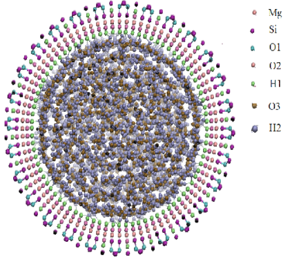
Figure 1: An initial configuration for simulation of water inside lizardite asbestos nanotube. $O1$ denotes oxygens in $SiO_{4}$ complexes, $O2$ - oxygens in hydroxyl groups and $O3$ water oxygen. $H1$ is hydrogen from $OH$ groups and $H2$ is water hydrogen.

We perform a set of molecular dynamics simulations of the system at different temperatures. Clay force field was used to simulate the asbestos atoms interactions clayff (Mg, Si, O1 for oxygen in $SiO_{4}$ groups, O2 for oxygens in $OH$ groups and H1 for hydrogens in $OH$). SPE/E model was employed for water. Cross interactions were obtained by Lorentz-Berthelot rule.

The system was periodic in z direction and confined in x and y ones. In order to perform calculation of coulombic forces we extend the simulation box in x and y directions from $X,Y_{min}=-73.19\AA$ up to $X,Y_{max}=73.19\AA$ with vacuum outside the tube and employ periodic boundary conditions in these directions too. No corrections on the vacuum slab were made for the sake of simplicity. We believe that these corrections are small and do not affect the qualitative behavior of the system.

During the simulations the atoms of the tube wall were held fixed although some simulations with free hydroxyl groups were also made for the sake of comparison. Later on we describe it in more details. Water molecules (and $OH$ groups when they were free to move) were considered as rigid bodies, i.e. the bond length and angles inside each body were fixed. The time step was set to $0.1fs$. The system was equilibrated for $1ns$ followed by propagation run of more $500ps$. In Refs. norman1 ; norman2 general methodology of selection of time step and the standards of molecular simulation are discussed.

We studied a wide range of temperatures starting from $T_{min}=300K$ up to $T_{max}=1000K$ with step $dT=100K$. The temperature was fixed by Nose-Hoover thermostat.

We also performed simulations of sodium chloride solvated in water confined in lyzardite asbestos fibers. For doing this we took an equilibrated structure of water inside the fiber and substituted randomly chosen water molecules by $20$ pairs of sodium and chlorine ions, i.e. the system contained $1760$ water molecules, $20$ sodium cations and $20$ chlorine anions which corresponds to concentration $0.7mol/kg$. The simulation setup for the system with salt was equivalent to the one of the pure water.

All simulations were performed using lammps simulation package lammps .

III III. Results and Discussion

III.1 Pure water

As an initial step we consider the lyzardite asbestos tube as being rigid, i.e. all atoms of the tube are fixed. We start the characterization of water behavior from the radial density profiles. The radial density is defined in the following way. Consider a cylindrical layer with internal radius $r$ and external one $r+dr$. The axis of the cylindrical layer coincides with the axis of the asbestos tube. Denote as $N(r)$ the number of water molecules inside the cylindrical layer. The position of the molecule is taken as the position of the oxygen atom. The volume of the layer is $V(r)=2\pi\left((r+dr)^{2}-r^{2}\right)\cdot H$. The radial number density is defined as $c(r)=N(r)/V(r)$ and the radial mass density is $\rho(r)=mN(r)/V(r)$ where $m=18a.e.$ is the mass of the water molecule. Below we use both radial mass density expressed in $g/cm^{3}$ and radial number density in $\AA^{-3}$.

Fig.  2 (a) shows a snapshot of the system at $T=500K$. One can see a set of very clear layers of water molecules, i.e. the density modulations. The strength of the modulations is as large as the radius of the tube. The internal radius of the tube is almost $9\AA$. Typically the density modulations spread for $2-3$ molecular diameters, i.e. in the case of asbestos fibers the modulations are stronger then usual. The density profiles for the temperatures from $T=300K$ up to $T=600K$ are shown in Fig.  2 (b).

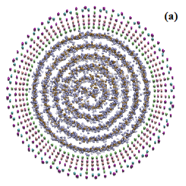
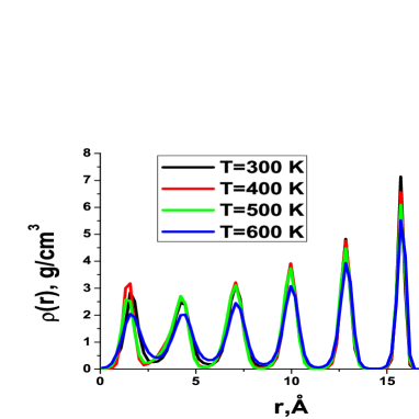
Figure 2: (a) Snapshot of the studied system at $T=500K$; (b) mass density distribution profiles at temperatures from $T=300K$ up to $T=600K$.

Figs.  3 (a) and (b) show a snapshot at $T=1000K$ and density profiles at temperatures from $T=700K$ up to $1000K$. One can see that even if the structure at $T=1000K$ is strongly smeared out it is still observable. It is even more clear from the density profiles shown in panel (b). One can conclude that asbestos fibers strongly modulate the density of water even at very high temperatures.

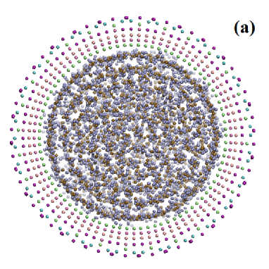
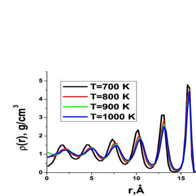
Figure 3: (a) Snapshot of the studied system at $T=1000K$; (b) mass density distribution profiles at temperatures from $T=700K$ up to $T=1000K$.

It is also important to see wheather there is any orientational order in different layers. Usually orientational ordering is characterized by Legender polynomial $P_{2}(cos\theta)=1.5cos^{2}(\theta)-0.5$, where $\theta$ is an angle characterizing the molecular orientation. We chose $\theta$ as the angle between a unit vector normal to the plane of a water molecule and the axis of the tube. Therefore if $\theta=0$ (the plane of the molecule is perpendicular to the axis of the tube) then $P_{2}(cos\theta)=1$. In the case of disordered orientation of the water molecules cancellation of different contributions takes place and $P_{2}=0$.

We study the radial distribution of $P_{2}(cos\theta)$ in the system. For doing this we calculate the $P_{2}$ parameter for each molecule in the layer extending from $r$ to $r+dr$ and then divide to the number of the molecules in the layer. The results are shown in Figs.  4 (a) and (b). The most pronounced orientational structure can be observed at $T=700K$. It demonstrates a peak and several minima. In order to understand it deeper let us compare the radial distribution of $P_{2}(cos\theta)$ with the radial distribution of the density at the same temperature (Fig.  5).

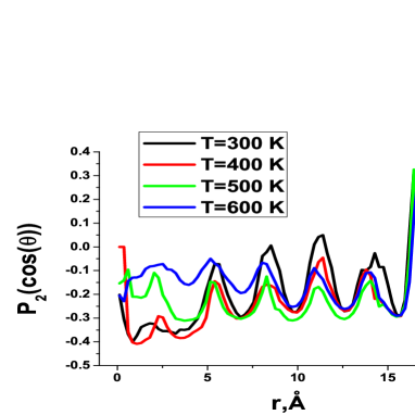
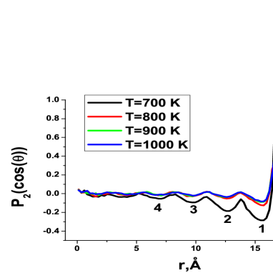
Figure 4: Radial distribution of Legender polynomial $P_{2}(cos\theta)$ (a) for lower temperatures and (b) for high temperatures. Numbers close to $T=700K$ curve in panel (b) numerate the minima at this temperature. The corresponding angles are shown in the right side of the figure.

In Fig.  5 we place these distributions one below another and draw thin lines representing the locations of the maxima of the density distribution. One can see that zero density corresponds to the large peak of $P_{2}$ close to the tube wall. It means that the peak can be related to tiny fluctuations of the density at this radius and most probably will be smeared out if the statistics is increased. At the same time all minima of the distribution of $P_{2}$ correspond to the maxima of the density distribution, i.e. the higher the density the more orientated structure is observed. It is in contrast with our recent observations of benzene confined into a carbon nanotube benzene-nanotube . From the height of the main peak of $P_{2}(r)$ distribution one can find that close to the wall the molecules are oriented to $23^{o}$ with respect to the tube axis.

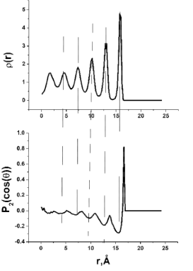
Figure 5: Comparison of the radial distribution of the density (top panel) and $P_{2}(cos\theta)$ (bottom panel) at $T=700K$. Thin solid lines show the location of the maxima of the density distribution.

At temperatures above $700K$ the orientational structure looks to be smeared out due to high temperature. At lower temperatures the structure looks odd. In order to understand it we need to consider the dynamics of the water molecules inside the asbestos tube.

Figs.  6 (a) and (b) show mean square displacements (MSD) in radial direction ($<x^{2}+y^{2}>$) and along the tube axis ($<z^{2}>$). One can see that at temperatures about $T=600K$ the dynamics of the system becomes extremely slow. Fig.  7 demonstrates the diffusion coefficient computed from MSD by Einstein relation. One can see that at $T=500K$ the diffusion coefficients become zero (for the sake of comparison we calculated the diffusion coefficient of bulk SPC/E water at $T=600K$: $D_{bulk}=2\cdot 10^{-8}m^{2}/s$, i.e. the diffusion coefficient of confined water is about $100$ times smaller). Therefore the system can be considered as being trapped in some state and cannot escape from it. It means that the results for $T\leq 600K$ are strongly affected by the initial configuration which was set random and therefore the low temperature results can be considered as some approach to the real behavior of the system but not as exact ones.

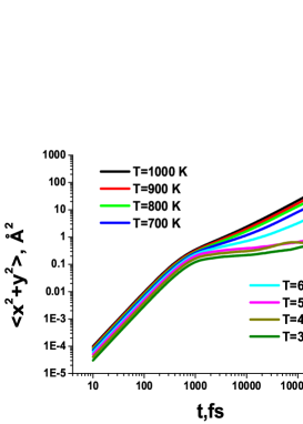
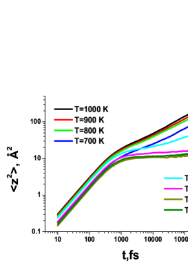
Figure 6: Mean square displacement of water molecules (a) in radial direction and (b) along the tube axis.

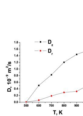
Figure 7: Diffusion coefficient of water confined in asbestos fiber. $D_{r}$ corresponds to the radial diffusion coefficient and $D_{z}$ to the diffusion along the tube axis.

In the present study we explore water in asbestos in the range of temperatures ranging from $300K$ up to $1000K$. It is known from experimental studies (see, for example, asb-degradation ) that asbestos is thermally degradable. The degradation of asbestos passes several stages. Firstly, water inside the fibers evaporates. At the second step the following chemical reaction takes place: $Mg_{3}Si_{2}O_{5}(OH)_{4}\longrightarrow Mg_{3}Si_{2}O_{7}+2H_{2}O$, i.e. asbestos looses the hydroxyl groups which form water and react with the rest of the tube. The water formed from the hydroxyl groups also evaporates. At the last step the system decomposes to a mixture of two magnesium silicates: $Mg_{2}SiO_{4}$ and $MgSiO_{3}$.

If we make the $OH$ groups free we can see thermal decomposition of asbestos at $T=500K$. We observe in our simulations that hydroxyl groups leave theirs places in the tube and go inside it. However, one cannot simulate chemical reactions in frames of classical force field like the one used here. Therefore the simulations with free $OH$ groups become unphysical at $T\geq 500K$, that is why we have to held the tube rigid.

In order to estimate the effect of the rigidity of the tube we perform some calculations of the properties of the system at $T=400K$ with free hydroxyl groups.

Fig.  8 (a) shows radial density profiles of water at $T=400K$ with fixed and free hydroxyl groups. One can see that in the case of free $OH$ groups the structure becomes more pronounced. Moreover, the positions of the peaks move toward the central axis of the tube. However, there is no strong qualitative differences between these cases.

Fig.  8 (b) demonstrates the mean square displacement (MSD) of water along the tube axis for fixed and free hydroxyl groups at $T=400K$. One can see that in the case of free $OH$ groups MSD becomes even smaller. As it was discussed above in the case of fixed hydroxyl groups we do not observe diffusive behavior in the time scale of our simulations. Therefore we do not observe it in the case of free $OH$ groups too.

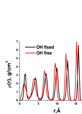
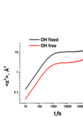
Figure 8: (a) Radial distribution of density of water inside the asbestos fiber with free and fixed $OH$ groups at $T=400K$; (b) mean square displacement along the tube axis for the same conditions.

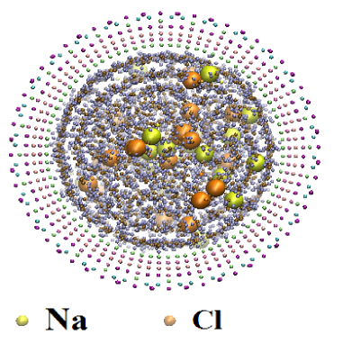
Figure 9: A snapshot of sodium chloride solution inside the asbestos fiber at $T=900K$.

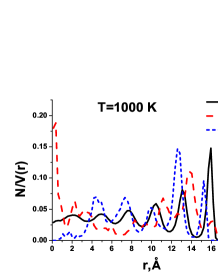
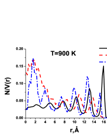
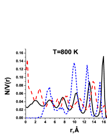
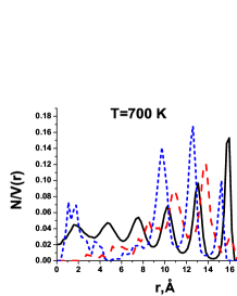
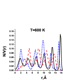
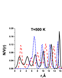
Figure 10: Radial density distribution of different species inside the asbestos fibers. Number density $N/V$ is used. In order to have all curves in the same scale we multiply the curves for sodium and chlorine to the factor $1760/20=88$.

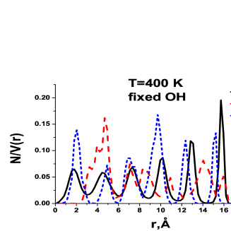
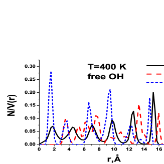
Figure 11: Radial density distribution of different species inside the asbestos fibers (a) with fixed $OH$ groups and (b) with free $OH$ groups. $T=400K$

In conclusion of this subsection we can see that the water dynamics inside the fibers is very slow and therefore we need to use very high temperatures (above $600K$). However, asbestos tube becomes unstable at such temperatures and we have to maintain it rigid during the simulations. Although it affects the results only small quantitative changes are detected. Therefore we believe that our results give reasonable qualitative description of the behavior of water inside the asbestos fibers.

III.2 Sodium Chloride solution inside the asbestos fiber

We proceed with study of sodium chloride solution inside the asbestos fibers. $40$ randomly chosen molecules of water were substituted by $Na^{+}$ and $Cl^{-}$ ion pairs and the behavior of the solution was studied. An example snapshot of the system is given in Fig.  9.

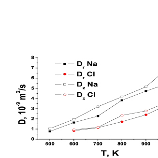
Figure 12: Diffusion coefficients of sodium and chlorine ions inside the asbestos fiber. Radial and along the tube axis coefficients are shown.

First, we study the radial density profiles of different species inside the tube and we do not observe any influence on the water structure inside the fibers due to sodium chloride introduction which means that the system can be considered as a solution.

The number density profiles of different species of the solution at different temperatures are shown in Fig.  10. One can see that the system demonstrates the layering of the species with different charges. For example, if one considers the case of $T=1000K$ the closest to the wall of the tube (large $r$) is the layer containing oxygens and chlorine ions, i.e. negatively charged species. The next layer is made of positively charged sodium. After that another oxygen and chlorine layer is observed and one more layer of sodium. At $r\leq 8\AA$ sodium ions do not show strong structuring while the densities of water and chlorine are still modulated. A peak of sodium is observed at the tube axis, however, this peak can be related to extremely small volume $V=2\pi r^{2}drH$ close to the tube axe and it can disappear in the thermodynamic limit.

Qualitatively similar picture is observed for other temperatures. As the temperature decreases the density modulations become more pronounced and at $T=600K$ all species demonstrate the density modulations in the whole range of $r$.

We also compare the density profiles in the case of fixed and free hydroxyl groups. The density profiles are shown in Fig.  11. One can see that like in the case of pure water, making $OH$ groups free makes the system more structured, but no strong qualitative changes appear. It allows us to conclude that the system with rigid tube leads to qualitatively correct behavior of the solution inside the fiber.

Fig.  12 shows the temperature dependence of radial and axial diffusion coefficient of sodium and chlorine. One can see that both sodium and chlorine have larger diffusion coefficients then water. The diffusion coefficients of sodium becomes zero at $T<500K$ and of chlorine at $T<600K$.

IV Conclusions

We consider the behavior of water and sodium chloride solution confined in lizardite asbestos nanotube which is a typical example of hydrophilic confinement. Confining water into asbestos tube strongly affects the dynamical properties. The diffusion coefficient drops about two orders of magnitude comparing to the bulk case. Like in the case of other hydrophilic pores water in asbestos tubes experiences vitrification rather then crystallization upon cooling. The density profiles are strongly affected by the geometry of the tube. The modulations of the density spread up to the whole tube region which is about $9\AA$.

In the case of sodium chloride solutions we observe clear double layer formation. It is shown that the closest to the wall of the tube is the layer containing oxygens and chlorine ions, i.e. negatively charged species while the next layer is made of positively charged sodium. At temperatures below $600K$ the density profiles demonstrate very sharp peaks, i.e. the solution becomes very structured in radial direction. It is interesting to note that both sodium and chlorine have larger diffusion coefficients then water.

- (1) C. Alba-Simionesco, B. Coasne, G. Dosseh, G. Dudziak, K. E. Gubbins, R. Radhakrishnan and M. Sliwinska-Bartkowiak, J. Phys.: Condens. Matter 18, R15 R68 (2006).
- (2) U. Gasser, J. Phys.: Condens. Matter 21, 203101 (2009).
- (3) S. A. Rice, Chem. Phys. Lett. 479, 1 (2009).
- (4) Yu. D. Fomin, J. Comput. Chem. 15, 2615 (2013).
- (5) Yu. D. Fomin, V. N. Ryzhov and E. N. Tsiok, J. Chem. Phys. 143, 184702 (2015).
- (6) A. I. Skoulidas, D. M. Ackerman, J. K. Johnson, D. S. Sholl, Phys. Rev. Lett. 89, 185901 (2002).
- (7) S. Jakobtorweihen, M. G. Verbeek, C. P. Lowe, F. J. Keil, B. Smit, Phys. Rev. Lett. 95, 044501 (2005).
- (8) H. Chen, J. K. Johnson, D. S. Sholl, J. Phys. Chem. B Lett. 110, 1971 (2006).
- (9) X. Qin, Q. Yuan, Y. Zhao, S. Xie, Z. Liu, Nanoletters 11, 2173 (2011).
- (10) M. Whitby, L. Cagnon, M. Thanou, N. Quirke, Nanoletters 8, 2632 (2008).
- (11) G. A. Mansoori and S. A. Rice, Advanced in Chemical Physics, 156, 197 (2014)
- (12) J. Bai, J. Wang, and X. C. Zeng, PNAS 103, 19664 (2006)
- (13) A. Alexiadis and S. Kassinos, Chem. Rev. 108, 5014 (2008).
- (14) A. Striolo, A. A. Chialvo, K. E. Gubbins, and P. T. Cummings, J. Chem. Phys. 122, 234712 (2005).
- (15) L. Liu, A. Faraone, C-Y. Mou, C-W. Yen and S-H. Chen, J. Phys.: Condens. Matter 16, S5403 S5436 (2004)
- (16) Ya. Zhang et al. PNAS, 108, 12206 (2011).
- (17) R. Renou, A. Szymczyk, and A. Ghoufi, J. Chem. Phys. 140, 044704 (2014).
- (18) F. G. Alabarse el al., Phys. Rev. Lett. 109, 035701 (2012).
- (19) E. Mamontov, Yu. A. Kumzerov, and S. B. Vakhrushev, Phys. Rev. E 71, 061502 (2005).
- (20) S. Durand-Vidal, J.P. Simonin and P. Turk, Electrolytes at Interfaces, Kluwer Academic Publisher (2002).
- (21) R. Renou et al., J. Phys. Chem. C, 117, 11017 (2013).
- (22) P. A. Bonnaud, B. Coasne and R. J.-M. Pellenq, J. Chem. Phys. 137, 064706 (2012).
- (23) D. Argyris, D. R. Cole and A. Striolo, ACS Nano, 4, p. 2035 (2010).
- (24) V. Marry, B. Rotenberg and P. Turq, Phys. Chem. Chem. Phys. 10, 4802 (2010).
- (25) S. Kerisit, Eu. S. Ilton and St. C. Parker, J. Phys. Chem. B 110, 20491 (2006).
- (26) L. Martinez, R. Andrade, E. G. Birgin, J. M. Martinez J. of Comput. Chem. 30(13), 2157 (2009).
- (27) R. T. Cygan, J.-J. Liang, and A. G. Kalinichev, J. Phys. Chem. B, 108, 1255 (2004).
- (28) G. E. Norman and V. V. Stegailov, Mathematical Models and Computer Simulations, 5, 305 (2013).
- (29) A. Y. Kuksin, I. V. Morozov, G. E. Norman, V. V. Stegailov and I. A. Valuev, Molecular Simulation, 31, 1005 (2005).
- (30) S. Plimpton, J. Comp. Phys, 117, 1-(1995), http://lammps.sandia.gov/index.html
- (31) Yu. D. Fomin, E. N. Tsiok and V. N. Ryzhov, J. Comp. Chem., 36, 901 (2015).
- (32) R. Kusiorowski, T. Zaremba, J. Piotrowski, J. Adamec, J. Therm. Anal. Calorim. 109, 693 (2012)