Nonchaotic evolution of triangular configuration due to gravitational radiation reaction in the three-body problem

Abstract

Continuing work initiated in an earlier publication [H. Asada, Phys. Rev. D 80, 064021 (2009)], the gravitational radiation reaction to Lagrange’s equilateral triangular solution of the three-body problem is investigated in an analytic method. The previous work is based on the energy balance argument, which is sufficient for a two-body system because the number of degrees of freedom (the semimajor axis and the eccentricity in quasi-Keplerian cases, for instance) equals that of the constants of motion such as the total energy and the orbital angular momentum. In a system with three (or more) bodies, however, the number of degrees of freedom is more than that of the constants of motion. Therefore, the present paper discusses the evolution of the triangular system by directly treating the gravitational radiation reaction force to each body. The perturbed equations of motion are solved by using the Laplace transform technique. It is found that the triangular configuration is adiabatically shrinking and is kept in equilibrium by increasing the orbital frequency due to the radiation reaction if the mass ratios satisfy the Newtonian stability condition. Long-term stability involving the first post-Newtonian corrections is also discussed.

I Introduction

The first direct detection of gravitational waves, named GW150914, has been achieved by Advanced LIGO GWPRL . In the near future, gravitational waves astronomy will be largely developed by a network of gravitational wave detectors such as Advanced VIRGO aVIRGO and KAGRA KAGRA . The test operation, named iKAGRA, has been started very recently as well as Advanced LIGO aLIGO . One of the most promising astrophysical sources is inspiraling and merging binary compact stars. In fact, the GW150914 event fits well with a binary black hole merger GWPRL . Numerical relativity has succeeded in simulating merging neutron stars and black holes (e.g. NR ). Analytical methods also have prepared accurate wave form templates for inspiraling compact binaries by the post-Newtonian approach PN and also by the black hole perturbations ST . A lot of effort is placed on bridging a gap between the inspiraling stage and the final merging phase (e.g., Damour ).

With growing interest, gravitational waves involving three-body interactions have been discussed (e.g., CIA ; GB ; Seto1 ; DSH ). Even the classical three-body (or $N$-body) problem in Newtonian gravity admits an increasing number of solutions; some of them express regular orbits and others are chaotic because the number of degrees of freedom of the system is more than that of conserved quantities. In particular, Lagrange’s equilateral triangular orbit has stimulated renewed interst for relativistic astrophysics THA ; Asada ; SM ; Schnittman ; IYA ; YA3 ; YTA ; BDEDSG . Very recently, a first relativistic hierarchical triple system has been discovered by Ransom and his collaborators Ransom . It has been pointed out by several authors that three-body interactions might play important roles for compact binary mergers in hierarchical triple systems BLS ; MH ; Wen ; Thompson ; Seto2 .

In binary systems, the evolution of the semimajor axis and the eccentricity is related to energy and orbital angular momentum losses due to the energy balance argument for the gravitational radiation at the second-and-a-half post-Newtonian (2.5PN) order. Thus, one can approximately calculate inspiraling of the binaries without directly solving the equation of motion. In the previous work Asada based on the energy balance argument, where Lagrange’s orbit is assumed to shrink and kept in an equilateral triangle, Asada has considered the three-body wave forms at the mass quadrupole, octupole, and current quadrupole orders, especially in an analytic method. By using the derived expressions, he has solved a gravitational wave inverse problem of determining the source parameters to the particular configuration (three masses, a distance of the source to an observer, and the orbital inclination angle to the line of sight) through observations of the gravitational wave forms alone. He has discussed also whether and how a binary source can be distinguished from a three-body system in Lagrange’s orbit or others and thus proposed a binary source test. Strictly speaking, however, the energy balance argument is not sufficient for three-body systems since the number of degrees of freedom in a system with three bodies is more than that of the constants of motion. Hence, one may think that the triangular orbit is likely to become chaotic owing to the gravitational radiation reaction. Is the key assumption in the previous work Asada correct?

Therefore, the main purpose of the present paper is to study whether the assumption in the previous work is correct. Namely, the evolution of the orbit is discussed through solving directly the equations of motion in order to avoid the energy balance argument for Lagrange’s orbit. In fact, even in Newtonian gravity without gravitational radiation, it is proved by Gascheau that Lagrange’s orbit is unstable Gascheau , unless

$$\frac{m_{1}m_{2}+m_{2}m_{3}+m_{3}m_{1}}{M^{2}}<\frac{1}{27},$$ (1)

where $m_{I}~{}(I=1,2,3)$ and $M=\sum m_{I}$ denote the mass of each body and the total mass, respectively. This stability condition has recently been corrected in the first post-Newtonian (1PN) approximation as YTA

$$\frac{m_{1}m_{2}+m_{2}m_{3}+m_{3}m_{1}}{M^{2}}+\frac{15}{2}\frac{m_{1}m_{2}m_{3}}{M^{3}}\lambda<\frac{1}{27}\left(1-\frac{391}{54}\lambda\right),$$ (2)

where we define

$$\lambda\equiv\left(\frac{GM\omega}{c^{3}}\right)^{2/3},$$ (3)

with the common orbital frequency $\omega$ of the system. Thus, the triangular configuration becomes less stable by the 1PN corrections. In order to investigate the effect of the gravitational radiation reaction on the evolution of the system, first, we focus on the Newtonian stable case that the condition (1) is satisfied. Next, we also discuss effects of the 1PN corrections on the stability by using Eq. (2).

This paper is organized as follows. In Sec. II, we briefly summarize Lagrange’s equilateral triangular orbit and derive the force by the gravitational radiation reaction. In Sec. III, we consider the evolution of the orbit due to the radiation reaction. Section IV is devoted to the discussion.

II Notation and Basic Formulation

II.1 Lagrange’s equilateral triangular solution

First, we consider the Newtonian gravity among three bodies in coplanar circular motion. By using a complex plane for orbital one, the location of each body is written as

$$z_{I}=r_{I}e^{i\theta_{I}},$$ (4)

where $r_{I}$ and $\theta_{I}$ are the field point distance and direction of the $I$th body. We choose the origin of the coordinates as the center of mass so that

$$m_{1}z_{1}+m_{2}z_{2}+m_{3}z_{3}=0,$$ (5)

and we denote the relative position between bodies $z_{IJ}\equiv z_{I}-z_{J}$ as

$$z_{IJ}=r_{IJ}e^{i\theta_{IJ}},$$ (6)

where $r_{IJ}$ and $\theta_{IJ}$ are the separation and the relative angle between the bodies, respectively. Hence, we have, with $I\neq J,J\neq K,K\neq I$,

$$r_{I}e^{i\theta_{I}}=\nu_{J}r_{IJ}e^{i\theta_{IJ}}+\nu_{K}r_{IK}e^{i\theta_{IK}},$$ (7)

where $\nu_{I}\equiv m_{I}/M$ is the mass ratio.

We consider an equilateral triangular configuration in equilibrium. Namely, we denote $r_{IJ}=\ell={\rm constant}$ and

$$\theta_{23}=\theta_{12}+\frac{2}{3}\pi,$$ (8)

$$\theta_{31}=\theta_{12}-\frac{2}{3}\pi.$$ (9)

Then, the equation of motion for $z_{IJ}$ becomes

$$\left(\frac{d\theta_{IJ}}{dt}\right)^{2}+i\frac{d^{2}\theta_{IJ}}{dt^{2}} =\frac{GM}{\ell^{3}}.$$ (10)

Thus, each body can move around the center of mass with the orbital frequency

$$\omega\equiv\frac{d\theta_{IJ}}{dt}=\sqrt{\frac{GM}{\ell^{3}}}.$$ (11)

By using Eqs. (7)–(9), we obtain

$$\bar{r}_{I}\equiv\frac{r_{I}}{\ell}=\sqrt{\nu_{J}^{2}+\nu_{J}\nu_{K}+\nu_{K}^{2}}.$$ (12)

In this paper, in order to investigate the effect of the gravitational radiation reaction on the evolution of the system, we focus on the case that the Newtonian equilateral triangle is stable, namely,

$$V\equiv\nu_{1}\nu_{2}+\nu_{2}\nu_{3}+\nu_{3}\nu_{1}<\frac{1}{27}.$$ (13)

II.2 Gravitational radiation reaction to Lagrange’s orbit

The reaction force due to the gravitational quadrupole radiation to the $I$th body per unit mass in the harmonic gauge is expressed as (see Appendix A)

$$F^{\rm RR}_{I}=-\frac{32}{5}\frac{GM}{\ell^{2}}\varepsilon\bar{r}_{I}[A_{I}+iB_{I}]e^{i\theta_{I}},$$ (14)

where we define

$$\varepsilon\equiv\left(\frac{GM\omega}{c^{3}}\right)^{5/3},$$ (15)

and

$$A_{I} \equiv\sum_{J}\nu_{J}(\bar{r}_{J})^{2}\sin(2\theta_{I}-2\theta_{J}),$$ (16)

$$B_{I} \equiv\sum_{J}\nu_{J}(\bar{r}_{J})^{2}\cos(2\theta_{I}-2\theta_{J}).$$ (17)

In the case of the equilateral triangular configuration, $\bar{r}_{J}$ and $\theta_{I}-\theta_{J}$ are constant, and hence, $A_{I}$ and $B_{I}$ in Eq. (14) are constant at the first order of $\varepsilon$. Moreover, one can show

$$\sum_{I}F^{\rm RR}_{I}=0.$$ (18)

It follows that the position of the center of mass is not changed by the reaction force. Using Eq. (7), the reaction force to $z_{IJ}$ is expressed as

$$F^{\rm RR}_{IJ} \equiv F^{\rm RR}_{I}-F^{\rm RR}_{J}$$

$$=\frac{16}{5}\frac{GM}{\ell^{2}}\varepsilon(A_{IJ}-iB_{IJ})e^{i\theta_{IJ}},$$ (19)

where

$$A_{IJ} =\sqrt{3}(\nu_{I}-\nu_{J})\nu_{K},$$ (20)

$$B_{IJ} =\nu_{I}(\nu_{J}-\nu_{K})+\nu_{J}(\nu_{K}-\nu_{I}).$$ (21)

III Evolution of Lagrange’s orbit

The motion of each body and that of the relative positions are perturbed due to gravitational radiation, while the position of the common center of mass and the orbital plane does not change. Therefore, the number of degrees of freedom for the perturbations in Lagrange’s orbit is 4. Let us consider the perturbation variables ($\chi_{12},X,\psi,\sigma$), so that

$$r_{12}=\ell \to\ell(1+\chi_{12}),$$ (22)

$$r_{31}=\ell \to\ell(1+\chi_{12}+X),$$ (23)

$$\varphi_{23}=\frac{\pi}{3} \to\frac{\pi}{3}+\psi,$$ (24)

$$\theta_{12}=\theta^{\rm N}_{12} \to\theta^{\rm N}_{12}+\sigma,$$ (25)

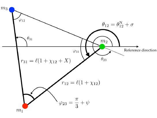
Figure 1: Perturbations in Lagrange’s orbit. Hence, $\chi_{12}$ and $\sigma$ correspond to the scale transformation of the triangle and the change of the angle of the system to a reference direction, respectively. On the other hand, $X$ and $\psi$ are the degrees of freedom of a shape change from the equilateral triangle.

where $\varphi_{23}$ denotes the opposite angle to $r_{23}$ and $\theta^{\rm N}_{12}$ is the Newtonian value (Fig. 1). In this choice of variables, $\chi_{12}$ and $\sigma$ correspond to the scale transformation of the triangle and the change of the angle of the system to a reference direction, respectively. On the other hand, $X$ and $\psi$ are the degrees of freedom of a shape change from the equilateral triangle. Therefore, the shrinking triangular configuration will adiabatically stay in equilibrium if and only if both $X$ and $\psi$ do not increase with time. We suppose that the order of magnitude of all the perturbations is $\varepsilon$.

The perturbed equations of motion are expressed as

$$\ddot{\chi}_{12}-3\chi_{12}-2\dot{\sigma}-\frac{9}{4}\nu_{3}X-\frac{3\sqrt{3}}{4}\nu_{3}\psi-\frac{16}{5}\varepsilon A_{12} =0,$$ (26)

$$2\dot{\chi}_{12}+\ddot{\sigma}-\frac{3\sqrt{3}}{4}\nu_{3}X+\frac{9}{4}\nu_{3}\psi+\frac{16}{5}\varepsilon B_{12} =0,$$ (27)

$$\ddot{\chi}_{12}-3\chi_{12}-2\dot{\sigma}+\ddot{X}-\left(3-\frac{9}{4}\nu_{2}\right)X-2\dot{\psi}-\frac{3\sqrt{3}}{4}\nu_{2}\psi-\frac{16}{5}\varepsilon A_{31} =0,$$ (28)

$$2\dot{\chi}_{12}+\ddot{\sigma}+2\dot{X}-\frac{3\sqrt{3}}{4}\nu_{2}X+\ddot{\psi}-\frac{9}{4}\nu_{2}\psi+\frac{16}{5}\varepsilon B_{31} =0,$$ (29)

where the dot denotes the derivative with respect to a normalized time $\bar{t}\equiv\omega t$. These equations do not contain $\sigma$. This is consistent with the fact that the initial value of $\sigma$ can be zero through the appropriate coordinate rotation. In order to avoid such a redundancy, let us use the perturbation in the orbital frequency $\omega$ as

$$\varpi\equiv\dot{\sigma},$$ (30)

instead of $\sigma$ as usual.

By solving Eqs. (26)–(29) (see Appendix B for more detail), we obtain

$$X =\frac{16}{45V}\varepsilon\left(3(\nu_{2}+\nu_{3})(A_{12}-A_{31})+\sqrt{3}(\nu_{2}-\nu_{3})(B_{12}-B_{31})\right)+X_{\rm(osc.)},$$ (31)

$$\psi =-\frac{16}{45V}\varepsilon\left(\sqrt{3}(\nu_{2}-\nu_{3})(A_{12}-A_{31})+(4-3\nu_{2}-3\nu_{3})(B_{12}-B_{31})\right)+\psi_{\rm(osc.)},$$ (32)

$$\chi_{12} =\frac{16}{5}\varepsilon\bar{t}\left[-2VB_{12}+\sqrt{3}\nu_{2}\nu_{3}(A_{12}-A_{31})+\nu_{3}(2-\nu_{2}-2\nu_{3})(B_{12}-B_{31})\right]$$

$$~{}~{}~{}+\frac{8}{45V}\varepsilon\left[18VA_{12}-3\nu_{3}(8-3\nu_{2}-6\nu_{3})(A_{12}-A_{31})+\sqrt{3}\nu_{3}(2+9\nu_{2})(B_{12}-B_{31})\right]$$

$$~{}~{}~{}+4\chi_{12\,{\rm(ini.)}}+2\varpi_{\rm(ini.)}+\frac{2(2-\nu_{2}-2\nu_{3})\nu_{3}}{V}X_{\rm(ini.)}-\frac{\sqrt{3}\nu_{2}\nu_{3}}{V}\dot{X}_{\rm(ini.)}$$

$$~{}~{}~{}+\frac{2\sqrt{3}\nu_{2}\nu_{3}}{V}\psi_{\rm(ini.)}+\frac{(2-\nu_{2}-2\nu_{3})\nu_{3}}{V}\dot{\psi}_{\rm(ini.)}+\chi_{12\,{\rm(osc.)}},$$ (33)

$$\varpi =-\frac{24}{5V}\varepsilon\bar{t}\left[-2VB_{12}+\sqrt{3}\nu_{2}\nu_{3}(A_{12}-A_{31})+\nu_{3}(2-\nu_{2}-2\nu_{3})(B_{12}-B_{31})\right]$$

$$~{}~{}~{}+\frac{16}{5V}\varepsilon\left(-2VA_{12}+\nu_{3}(2-\nu_{2}-2\nu_{3})(A_{12}-A_{31})-\sqrt{3}\nu_{2}\nu_{3}(B_{12}-B_{31})\right)$$

$$~{}~{}~{}-\frac{3}{2}\left(4\chi_{12\,{\rm(ini.)}}+2\varpi_{\rm(ini.)}+\frac{2\nu_{3}(2-\nu_{2}-2\nu_{3})}{V}X_{\rm(ini.)}-\frac{\sqrt{3}\nu_{2}\nu_{3}}{V}\dot{X}_{\rm(ini.)}\right.$$

$$~{}~{}~{}\left.+\frac{2\sqrt{3}\nu_{2}\nu_{3}}{V}\psi_{\rm(ini.)}+\frac{\nu_{3}(2-\nu_{2}-2\nu_{3})}{V}\dot{\psi}_{\rm(ini.)}\right)+\varpi_{\rm(osc.)},$$ (34)

where the subscript (ini.) denotes the initial value and $X_{\rm(osc.)}$, $\psi_{\rm(osc.)}$, $\chi_{12\,{\rm(osc.)}}$, and $\varpi_{\rm(osc.)}$ are oscillating terms expressed as

$$X_{\rm(osc.)} =\frac{1}{(\alpha-\beta)(\alpha+\beta)}\left[\left(\alpha^{2}-4+\frac{9}{4}(\nu_{2}+\nu_{3})\right)X_{\rm(ini.)}-\frac{3\sqrt{3}}{4}(\nu_{2}-\nu_{3})\psi_{\rm(ini.)}-2\dot{\psi}_{\rm(ini.)}\right.$$

$$~{}~{}~{}\left.+\frac{16}{5\alpha^{2}}\varepsilon\left(\left[\alpha^{2}+\frac{9}{4}(\nu_{2}+\nu_{3})\right](A_{12}-A_{31})+\frac{3\sqrt{3}}{4}(\nu_{2}-\nu_{3})(B_{12}-B_{31})\right)\right]\cos(\alpha\bar{t})$$

$$~{}~{}~{}-\frac{1}{(\alpha-\beta)(\alpha+\beta)}\left[\left(\beta^{2}-4+\frac{9}{4}(\nu_{2}+\nu_{3})\right)X_{\rm(ini.)}-\frac{3\sqrt{3}}{4}(\nu_{2}-\nu_{3})\psi_{\rm(ini.)}-2\dot{\psi}_{\rm(ini.)}\right.$$

$$~{}~{}~{}\left.+\frac{16}{5\beta^{2}}\varepsilon\left(\left[\beta^{2}+\frac{9}{4}(\nu_{2}+\nu_{3})\right](A_{12}-A_{31})+\frac{3\sqrt{3}}{4}(\nu_{2}-\nu_{3})(B_{12}-B_{31})\right)\right]\cos(\beta\bar{t})$$

$$~{}~{}~{}-\frac{1}{\alpha(\alpha-\beta)(\alpha+\beta)}\left[\frac{3\sqrt{3}}{4}(\nu_{2}-\nu_{3})(2X_{\rm(ini.)}+\dot{\psi}_{\rm(ini.)})-\alpha^{2}\dot{X}_{\rm(ini.)}\right.$$

$$~{}~{}~{}\left.-\frac{9}{4}(\nu_{2}+\nu_{3})(\dot{X}_{\rm(ini.)}-2\psi_{\rm(ini.)})+\frac{32}{5}\varepsilon(B_{12}-B_{31})\right]\sin(\alpha\bar{t})$$

$$~{}~{}~{}+\frac{1}{\beta(\alpha-\beta)(\alpha+\beta)}\left[\frac{3\sqrt{3}}{4}(\nu_{2}-\nu_{3})(2X_{\rm(ini.)}+\dot{\psi}_{\rm(ini.)})-\beta^{2}\dot{X}_{\rm(ini.)}\right.$$

$$~{}~{}~{}\left.-\frac{9}{4}(\nu_{2}+\nu_{3})(\dot{X}_{\rm(ini.)}-2\psi_{\rm(ini.)})+\frac{32}{5}\varepsilon(B_{12}-B_{31})\right]\sin(\beta\bar{t}),$$ (35)

$$\psi_{\rm(osc.)} =-\frac{1}{(\alpha-\beta)(\alpha+\beta)}\left[\frac{3\sqrt{3}}{4}(\nu_{2}-\nu_{3})X_{\rm(ini.)}-2\dot{X}_{\rm(ini.)}-\left(\alpha^{2}-1-\frac{9}{4}(\nu_{2}+\nu_{3})\right)\psi_{\rm(ini.)}\right.$$

$$~{}~{}~{}+\left.\frac{16}{5\alpha^{2}}\varepsilon\left(\frac{3\sqrt{3}}{4}(\nu_{2}-\nu_{3})(A_{12}-A_{31})+\left[\alpha^{2}+3-\frac{9}{4}(\nu_{2}+\nu_{3})\right](B_{12}-B_{31})\right)\right]\cos(\alpha\bar{t})$$

$$~{}~{}~{}+\frac{1}{(\alpha-\beta)(\alpha+\beta)}\left[\frac{3\sqrt{3}}{4}(\nu_{2}-\nu_{3})X_{\rm(ini.)}-2\dot{X}_{\rm(ini.)}-\left(\beta^{2}-1-\frac{9}{4}(\nu_{2}+\nu_{3})\right)\psi_{\rm(ini.)}\right.$$

$$~{}~{}~{}+\left.\frac{16}{5\beta^{2}}\varepsilon\left(\frac{3\sqrt{3}}{4}(\nu_{2}-\nu_{3})(A_{12}-A_{31})+\left[\beta^{2}+3-\frac{9}{4}(\nu_{2}+\nu_{3})\right](B_{12}-B_{31})\right)\right]\cos(\beta\bar{t})$$

$$~{}~{}~{}+\frac{1}{\alpha(\alpha-\beta)(\alpha+\beta)}\left[\left(3-\frac{9}{4}(\nu_{2}+\nu_{3})\right)(2X_{\rm(ini.)}+\dot{\psi}_{\rm(ini.)})\right.$$

$$~{}~{}~{}\left.-\frac{3\sqrt{3}}{4}(\nu_{2}-\nu_{3})(\dot{X}_{\rm(ini.)}-2\psi_{\rm(ini.)})+\alpha^{2}\dot{\psi}_{\rm(ini.)}-\frac{32}{5}\varepsilon(A_{12}-A_{31})\right]\sin(\alpha\bar{t})$$

$$~{}~{}~{}-\frac{1}{\beta(\alpha-\beta)(\alpha+\beta)}\left[\left(3-\frac{9}{4}(\nu_{2}+\nu_{3})\right)(2X_{\rm(ini.)}+\dot{\psi}_{\rm(ini.)})\right.$$

$$~{}~{}~{}\left.-\frac{3\sqrt{3}}{4}(\nu_{2}-\nu_{3})(\dot{X}_{\rm(ini.)}-2\psi_{\rm(ini.)})+\beta^{2}\dot{\psi}_{\rm(ini.)}-\frac{32}{5}\varepsilon(A_{12}-A_{31})\right]\sin(\beta\bar{t}),$$ (36)

$$\chi_{12\,{\rm(osc.)}} =-\left[3\chi_{12\,{\rm(ini.)}}+2\varpi_{\rm(ini.)}-\frac{1}{2V}\left(-\nu_{3}(2\nu_{1}+\nu_{2})(3X_{\rm(ini.)}+2\dot{\psi}_{\rm(ini.)})+\sqrt{3}\nu_{2}\nu_{3}(2\dot{X}_{\rm(ini.)}-3\psi_{\rm(ini.)})\right)\right.$$

$$~{}~{}~{}\left.+\frac{8}{5V}\varepsilon\left(2VA_{12}-\nu_{3}(2\nu_{1}+\nu_{2})(A_{12}-A_{31})+\sqrt{3}\nu_{2}\nu_{3}(B_{12}-B_{31})\right)\right]\cos\bar{t}$$

$$~{}~{}~{}+\left[\dot{\chi}_{12\,{\rm(ini.)}}+\frac{1}{2V}\left(\nu_{3}(2\nu_{1}+\nu_{2})\dot{X}_{\rm(ini.)}+\sqrt{3}\nu_{2}\nu_{3}\dot{\psi}_{\rm(ini.)}\right)\right.$$

$$~{}~{}~{}\left.+\frac{16}{5V}\varepsilon\left(2VB_{12}-\sqrt{3}\nu_{2}\nu_{3}(A_{12}-A_{31})-\nu_{3}(2\nu_{1}+\nu_{2})(B_{12}-B_{31})\right)\right]\sin\bar{t}$$

$$~{}~{}~{}+\frac{\sqrt{3}}{18(\alpha-\beta)(\alpha+\beta)V}$$

$$~{}~{}~{}\times\left[\sqrt{3}\alpha^{2}\nu_{3}(2\alpha^{2}-8+3\nu_{2}+6\nu_{3})X_{\rm(ini.)}+6\sqrt{3}\nu_{3}(2-\nu_{2}-2\nu_{3})(2X_{\rm(ini.)}+\dot{\psi}_{\rm(ini.)})\right.$$

$$~{}~{}~{}-18\nu_{2}\nu_{3}(\dot{X}_{\rm(ini.)}-2\psi_{\rm(ini.)})+\alpha^{2}\nu_{3}(2\alpha^{2}-2-9\nu_{2})\psi_{\rm(ini.)}$$

$$~{}~{}~{}+\left.\frac{16}{5}\varepsilon\left(\sqrt{3}\nu_{3}(2\alpha^{2}-8+3\nu_{2}+6\nu_{3})(A_{12}-A_{31})-\nu_{3}(2\alpha^{2}-2-9\nu_{2})(B_{12}-B_{31})\right)\right]\cos(\alpha\bar{t})$$

$$~{}~{}~{}-\frac{\sqrt{3}}{18(\alpha-\beta)(\alpha+\beta)V}$$

$$~{}~{}~{}\times\left[\sqrt{3}\beta^{2}\nu_{3}(2\beta^{2}-8+3\nu_{2}+6\nu_{3})X_{\rm(ini.)}+6\sqrt{3}\nu_{3}(2\nu_{1}+\nu_{2})(2X_{\rm(ini.)}+\dot{\psi}_{\rm(ini.)})\right.$$

$$~{}~{}~{}-18\nu_{2}\nu_{3}(\dot{X}_{\rm(ini.)}-2\psi_{\rm(ini.)})+\beta^{2}\nu_{3}(2\beta^{2}-2-9\nu_{2})\psi_{\rm(ini.)}$$

$$~{}~{}~{}+\left.\frac{16}{5}\varepsilon\left(\sqrt{3}\nu_{3}(2\beta^{2}-8+3\nu_{2}+6\nu_{3})(A_{12}-A_{31})-\nu_{3}(2\beta^{2}-2-9\nu_{2})(B_{12}-B_{31})\right)\right]\cos(\beta\bar{t})$$

$$~{}~{}~{}-\frac{\sqrt{3}}{18\alpha(\alpha-\beta)(\alpha+\beta)V}$$

$$~{}~{}~{}\times\left[\frac{27V}{2}\nu_{3}\left((2X_{\rm(ini.)}+\dot{\psi}_{\rm(ini.)})+\sqrt{3}(\dot{X}_{\rm(ini.)}-2\psi_{\rm(ini.)})\right)\right.$$

$$~{}~{}~{}\left.+3\sqrt{3}\alpha^{2}\nu_{3}(2-\nu_{2}-2\nu_{3})\dot{X}_{\rm(ini.)}+9\alpha^{2}\nu_{2}\nu_{3}\dot{\psi}_{\rm(ini.)}\right.$$

$$~{}~{}~{}\left.-\frac{96\sqrt{3}}{5}\nu_{3}\varepsilon\left(\sqrt{3}\nu_{2}(A_{12}-A_{31})+(2-\nu_{2}-2\nu_{3})(B_{12}-B_{31})\right)\right]\sin(\alpha\bar{t})$$

$$~{}~{}~{}+\frac{\sqrt{3}}{18\beta(\alpha-\beta)(\alpha+\beta)V}$$

$$~{}~{}~{}\times\left[\frac{27V}{2}\nu_{3}\left((2X_{\rm(ini.)}+\dot{\psi}_{\rm(ini.)})+\sqrt{3}(\dot{X}_{\rm(ini.)}-2\psi_{\rm(ini.)})\right)\right.$$

$$~{}~{}~{}\left.+3\sqrt{3}\beta^{2}\nu_{3}(2\nu_{1}+\nu_{2})\dot{X}_{\rm(ini.)}+9\beta^{2}\nu_{2}\nu_{3}\dot{\psi}_{\rm(ini.)}\right.$$

$$~{}~{}~{}\left.-\frac{96\sqrt{3}}{5}\nu_{3}\varepsilon\left(\sqrt{3}\nu_{2}(A_{12}-A_{31})+(2-\nu_{2}-2\nu_{3})(B_{12}-B_{31})\right)\right]\sin(\beta\bar{t}),$$ (37)

$$\varpi_{\rm(osc.)} =2\left[3\chi_{12\,{\rm(ini.)}}+2\varpi_{\rm(ini.)}-\frac{1}{2V}\left(-\nu_{3}(2\nu_{1}+\nu_{2})(3X_{\rm(ini.)}+2\dot{\psi}_{\rm(ini.)})+\sqrt{3}\nu_{2}\nu_{3}(2\dot{X}_{\rm(ini.)}-3\psi_{\rm(ini.)})\right)\right.$$

$$~{}~{}~{}\left.+\frac{8}{5V}\varepsilon\left(2VA_{12}-\nu_{3}(2\nu_{1}+\nu_{2})(A_{12}-A_{31})+\sqrt{3}\nu_{2}\nu_{3}(B_{12}-B_{31})\right)\right]\cos\bar{t}$$

$$~{}~{}~{}-2\left[\dot{\chi}_{12\,{\rm(ini.)}}+\frac{1}{2V}\left(\nu_{3}(2\nu_{1}+\nu_{2})\dot{X}_{\rm(ini.)}+\sqrt{3}\nu_{2}\nu_{3}\dot{\psi}_{\rm(ini.)}\right)\right.$$

$$~{}~{}~{}\left.+\frac{16}{5V}\varepsilon\left(2VB_{12}-\sqrt{3}\nu_{2}\nu_{3}(A_{12}-A_{31})-\nu_{3}(2\nu_{1}+\nu_{2})(B_{12}-B_{31})\right)\right]\sin\bar{t}$$

$$~{}~{}~{}+\frac{\sqrt{3}}{18(\alpha-\beta)(\alpha+\beta)V}\left[-\sqrt{3}\nu_{3}\left[2\alpha^{4}-2\alpha^{2}+27(2\nu_{1}+\nu_{2})\right](2X_{\rm(ini.)}+\dot{\psi}_{\rm(ini.)})+9\alpha^{2}\nu_{2}\nu_{3}\dot{X}_{\rm(ini.)}\right.$$

$$~{}~{}~{}+\nu_{3}(2\alpha^{4}-2\alpha^{2}+27\nu_{2})(\dot{X}_{\rm(ini.)}-2\psi_{\rm(ini.)})-3\sqrt{3}\alpha^{2}\nu_{3}(2\nu_{1}+\nu_{2})\dot{\psi}_{\rm(ini.)}$$

$$~{}~{}~{}\left.+\frac{96\sqrt{3}}{5}\nu_{3}\varepsilon\left((2\nu_{1}+\nu_{2})(A_{12}-A_{31})-\sqrt{3}\nu_{2}(B_{12}-B_{31})\right)\right]\cos(\alpha\bar{t})$$

$$~{}~{}~{}-\frac{\sqrt{3}}{18(\alpha-\beta)(\alpha+\beta)V}\left[-\sqrt{3}\nu_{3}\left[2\beta^{4}-2\beta^{2}+27(2\nu_{1}+\nu_{2})\right](2X_{\rm(ini.)}+\dot{\psi}_{\rm(ini.)})+9\beta^{2}\nu_{2}\nu_{3}\dot{X}_{\rm(ini.)}\right.$$

$$~{}~{}~{}+\nu_{3}(2\beta^{4}-2\beta^{2}+27\nu_{2})(\dot{X}_{\rm(ini.)}-2\psi_{\rm(ini.)})-3\sqrt{3}\beta^{2}\nu_{3}(2\nu_{1}+\nu_{2})\dot{\psi}_{\rm(ini.)}$$

$$~{}~{}~{}\left.+\frac{96\sqrt{3}}{5}\nu_{3}\varepsilon\left((2-\nu_{2}-2\nu_{3})(A_{12}-A_{31})-\sqrt{3}\nu_{2}(B_{12}-B_{31})\right)\right]\cos(\beta\bar{t})$$

$$~{}~{}~{}+\frac{\sqrt{3}}{18\alpha(\alpha-\beta)(\alpha+\beta)V}\left[\frac{27}{4}V\nu_{3}\left((2\alpha^{2}+9\nu_{2})X_{\rm(ini.)}-\sqrt{3}(2\alpha^{2}+6-3\nu_{2}-6\nu_{3})\psi_{\rm(ini.)}\right)\right.$$

$$~{}~{}~{}+6\sqrt{3}\alpha^{2}\nu_{3}(2-\nu_{2}-2\nu_{3})\dot{X}_{\rm(ini.)}+18\alpha^{2}\nu_{2}\nu_{3}\dot{\psi}_{\rm(ini.)}$$

$$~{}~{}~{}-\frac{16}{5}\nu_{3}\varepsilon\left(\left[2\alpha^{4}-(2-9\nu_{2})\alpha^{2}+27\nu_{2}\right](A_{12}-A_{31})\right.$$

$$~{}~{}~{}\left.\left.+\sqrt{3}\left[2\alpha^{4}+(4-3\nu_{2}-6\nu_{3})\alpha^{2}+9(2\nu_{1}+\nu_{2})\right](B_{12}-B_{31})\right)\right]\sin(\alpha\bar{t})$$

$$~{}~{}~{}-\frac{\sqrt{3}}{18\beta(\alpha-\beta)(\alpha+\beta)V}\left[\frac{27}{4}V\nu_{3}\left((2\beta^{2}+9\nu_{2})X_{\rm(ini.)}-\sqrt{3}(2\beta^{2}+6-3\nu_{2}-6\nu_{3})\psi_{\rm(ini.)}\right)\right.$$

$$~{}~{}~{}+6\sqrt{3}\beta^{2}\nu_{3}(2\nu_{1}+\nu_{2})\dot{X}_{\rm(ini.)}+18\beta^{2}\nu_{2}\nu_{3}\dot{\psi}_{\rm(ini.)}$$

$$~{}~{}~{}-\frac{16}{5}\nu_{3}\varepsilon\left(\left[2\beta^{4}-(2-9\nu_{2})\beta^{2}+27\nu_{2}\right](A_{12}-A_{31})\right.$$

$$~{}~{}~{}\left.\left.+\sqrt{3}\left[2\beta^{4}+(4-3\nu_{2}-6\nu_{3})\beta^{2}+9(2\nu_{1}+\nu_{2})\right](B_{12}-B_{31})\right)\right]\sin(\beta\bar{t}),$$ (38)

with $\alpha\equiv\sqrt{(1+\sqrt{1-27V})/2}$ and $\beta\equiv\sqrt{(1-\sqrt{1-27V})/2}$.

Equations (31) and (32) mean that the perturbations $X$ and $\psi$ do not increase with time but oscillate around some values. As mentioned already, the triangular configuration will adiabatically shrink and be kept in equilibrium.

On the other hand, $\chi_{12}$ corresponding to the scale transformation of the system includes a linear term in time as

$$\chi_{12}^{(t)}\equiv\frac{16}{5}\varepsilon\left[-2VB_{12}+\sqrt{3}\nu_{2}\nu_{3}(A_{12}-A_{31})+\nu_{3}(2-\nu_{2}-2\nu_{3})(B_{12}-B_{31})\right].$$ (39)

Hence, the triangle changes with time as a similarity transformation. From Eqs. (20) and (21), we obtain

$$\chi_{12}^{(t)} =-\frac{64}{5V}\varepsilon\left(\nu_{1}^{2}\nu_{2}^{2}+\nu_{2}^{2}\nu_{3}^{2}+\nu_{3}^{2}\nu_{1}^{2}-\nu_{1}^{2}\nu_{2}\nu_{3}-\nu_{1}\nu_{2}^{2}\nu_{3}-\nu_{1}\nu_{2}\nu_{3}^{2}\right)$$

$$=-\frac{32}{5V}\varepsilon\left[\nu_{1}^{2}(\nu_{2}-\nu_{3})^{2}+\nu_{2}^{2}(\nu_{3}-\nu_{1})^{2}+\nu_{3}^{2}(\nu_{1}-\nu_{2})^{2}\right]$$

$$\leq 0,$$ (40)

where the equality holds if and only if $\nu_{1}=\nu_{2}=\nu_{3}=1/3$. In this equality case, the size of triangle does not change. This is because gravitational waves are not emitted from the triangular configuration as a consequence of a complete phase cancellation of the waves in the quadrupole approximation when $\nu_{1}=\nu_{2}=\nu_{3}=1/3$ [see Eqs. (20) and (21)]. For the Newtonian stable case as in Eq. (13), one can obtain $\chi_{12}^{(t)}<0$. Moreover, the perturbation $\varpi$ in the orbital frequency also has a linear term in time as

$$\varpi^{(t)} \equiv-\frac{24}{5V}\varepsilon\left[-2VB_{12}+\sqrt{3}\nu_{2}\nu_{3}(A_{12}-A_{31})+\nu_{3}(2-\nu_{2}-2\nu_{3})(B_{12}-B_{31})\right]$$

$$=-\frac{3}{2}\chi_{12}^{(t)}$$

$$\geq 0.$$ (41)

Substituting this into the first term of Eq. (34), one can see that the system shrinks with increasing the orbital frequency linearly in the normalized time $\bar{t}\equiv\omega t$.

Before closing this section, let us discuss the effects of the 1PN corrections on the long-term stability. In the long time evolution, the 1PN corrections to this triple system will not be negligible. In fact, it has been implied that for some mass ratios, even if the Newtonian is stable, the triangular configuration in the restricted three-body problem may break up as its final fate SM . Hence, it is worthwhile to study the long-term stability for three finite masses. After a long time (i.e. $\bar{t}\gg 1$), the perturbation in the orbital frequency $\varpi$ increases, where the linear term in time $\varpi^{(t)}$ dominates and the others become negligible. Therefore, the orbital frequency can be rewritten as

$$\omega\simeq\omega_{\rm(ini.)}(1+\varpi^{(t)}\bar{t}).$$ (42)

Figure 2 shows a contour map of the critical values of $\lambda$, which are marginal points of Eq. (2), as a function of $\nu_{2}$ and $\nu_{3}$. Note that since Eq. (2) is valid only for small values of $\lambda$, the lower-left region of Fig. 2 may not be accurate. Indeed, one can see $V<\lambda$ in this region; thus, the critical values of $\lambda$ are very sensitive to higher PN corrections.

We also perform numerical tests with an adiabatic treatment for two cases of initial values. Case 1: $\nu_{1}=0.973,~{}~{}\nu_{2}=0.027,~{}~{}\nu_{3}=0,~{}~{}\lambda_{\rm(ini.)}=1/200$, which use the same values in Fig. 3 of Ref. SM . Case 2: $\nu_{1}=0.98,~{}~{}\nu_{2}=0.01,~{}~{}\nu_{3}=0.01,~{}~{}\lambda_{\rm(ini.)}=1/200$. In case 1, the system becomes unstable with $\bar{t}\sim 10^{5}$ and $\lambda_{\rm(fin.)}\approx 1/25$. This is consistent with the result in Ref. SM . In case 2, the system becomes unstable with $\bar{t}\sim 10^{6}$ and $\lambda_{\rm(fin.)}\approx 1/15$. These results are in agreement with Fig. 2. In both cases, the systems, which are initially stable, become unstable in the final states. Therefore, it is unlikely that the triangular configuration shrinks to merge. However, in such final states where $\lambda_{\rm(fin.)}\sim 0.1$, it is necessary to incorporate the higher order PN corrections. Moreover, it has been pointed out that even for binary systems the PN approximation may be no longer valid in such a region YB ; SFN . Therefore, we need another approach, which is valid in strong fields, in order to investigate the stability of the system more precisely.

IV Conclusion

We have investigated the gravitational radiation reaction to Lagrange’s equilateral triangular orbit. It has been found that the triangular configuration is adiabatically shrinking and kept in equilibrium with increasing the orbital frequency at the 2.5PN order if the mass ratios satisfy the Newtonian stability condition as in Eq. (1). These results support the assumption in Ref. Asada , where Lagrange’s orbit shrinks and remains an equilateral triangle. Therefore, it may be possible to distinguish a binary source from a three-body system in Lagrange’s orbit or others by using Asada’s method as a binary source test.

We have also discussed long-term stability involving the 1PN corrections and shown that the triangular configuration, which is initially stable, will become unstable in the final states where $\lambda_{\rm(fin.)}\sim 0.1$. It is left as a future work to investigate the dynamics of the three bodies more precisely.

Appendix A A DERIVATION OF GRAVITATIONAL RADIATION REACTION FORCE

The 2.5PN correction to the metric $h^{Q}_{00}$ in the harmonic gauge is MTW ; Maggiore ; Blanchet

$$h^{Q}_{00}=-\frac{2\Phi}{c^{2}},$$ (43)

where

$$\Phi\equiv\frac{G}{5c^{5}}\frac{d^{5}Q_{ij}}{dt^{5}}x^{i}x^{j}$$ (44)

is the correction to the Newtonian potential with the mass quadrupole moment

$$Q_{ij}\equiv\int\rho\left(x_{i}x_{j}-\frac{1}{3}\delta_{ij}r^{2}\right)d^{3}x.$$ (45)

Thus, the quadrupole radiation reaction force per unit mass is

$$F_{i}^{\rm RR}=-\frac{\partial\Phi}{\partial x^{i}}.$$ (46)

We consider Lagrange’s orbit of the three bodies on the $(x,y)$ plane, where nonzero components of the quadrupole moment $Q_{ij}$ are

$$Q_{xx} =\sum_{J}m_{J}\left(r_{J}\right)^{2}\cos^{2}\theta_{J}+{\rm constant},$$ (47)

$$Q_{xy} =Q_{yx}=\sum_{J}m_{J}\left(r_{J}\right)^{2}\cos\theta_{J}\sin\theta_{J},$$ (48)

$$Q_{yy} =\sum_{J}m_{J}\left(r_{J}\right)^{2}\sin^{2}\theta_{J}+{\rm constant},$$ (49)

$$Q_{zz} ={\rm constant}.$$ (50)

Therefore, one can see

$$F_{z}^{\rm RR}\propto\frac{d^{5}Q_{zk}}{dt^{5}}x^{k}=\frac{d^{5}Q_{zz}}{dt^{5}}x^{z}=0.$$ (51)

It follows that the orbital plane is not changed by the radiation reaction, and hence, we focus on the $(x,y)$ plane in the following.

The reaction force (46) on a field point $\boldsymbol{r}=r(\cos\theta,\sin\theta)$ can be expressed as

$$\boldsymbol{F}^{\rm RR} =\frac{32}{5}\frac{Gr\omega^{5}}{c^{5}}\sum_{J}m_{J}r_{J}^{2}\begin{bmatrix}\sin(2\theta_{J})&-\cos(2\theta_{J})\\ -\cos(2\theta_{J})&-\sin(2\theta_{J})\end{bmatrix}\begin{bmatrix}\cos\theta\\ \sin\theta\end{bmatrix}$$

$$=\frac{32}{5}\frac{Gr\omega^{5}}{c^{5}}\sum_{J}m_{J}r_{J}^{2}\begin{bmatrix}\sin(2\theta_{J}-2\theta)&\cos(2\theta_{J}-2\theta)\\ -\cos(2\theta_{J}-2\theta)&\sin(2\theta_{J}-2\theta)\end{bmatrix}\begin{bmatrix}\cos\theta\\ \sin\theta\end{bmatrix}.$$ (52)

By replacing $r$ and $\theta$ with $r_{I}$ and $\theta_{I}$, respectively, the force to the $I$th body per unit mass is

$$F^{\rm RR}_{I}=-\frac{32}{5}\frac{GM}{\ell^{2}}\varepsilon\bar{r}_{I}[A_{I}+iB_{I}]e^{i\theta_{I}},$$ (53)

where we define

$$\varepsilon\equiv\left(\frac{GM\omega}{c^{3}}\right)^{5/3},$$ (54)

and

$$A_{I} \equiv\sum_{J}\nu_{J}(\bar{r}_{J})^{2}\sin(2\theta_{I}-2\theta_{J}),$$ (55)

$$B_{I} \equiv\sum_{J}\nu_{J}(\bar{r}_{J})^{2}\cos(2\theta_{I}-2\theta_{J}).$$ (56)

Appendix B SOLVING THE EQUATIONS OF MOTION FOR PERTURBATIONS

In order to solve Eqs. (26)–(29), let us take the Laplace transform as

$$F(s)\equiv\mathscr{L}[f(t)]=\int_{0}^{\infty}e^{-st}f(t)dt.$$ (57)

Thus, the perturbed equations of motion (26)–(29) become

$$(s^{2}-3)L_{12}-s\chi_{12\,{\rm(ini.)}}-\dot{\chi}_{12\,{\rm(ini.)}}-2L_{\varpi}-\frac{9}{4}\nu_{3}L_{X}-\frac{3\sqrt{3}}{4}\nu_{3}L_{\psi}-\frac{16}{5}\varepsilon A_{12}\frac{1}{s} =0,$$ (58)

$$2sL_{12}-2\chi_{12\,{\rm(ini.)}}+sL_{\varpi}-\varpi_{\rm(ini.)}-\frac{3\sqrt{3}}{4}\nu_{3}L_{X}+\frac{9}{4}\nu_{3}L_{\psi}+\frac{16}{5}\varepsilon B_{12}\frac{1}{s} =0,$$ (59)

$$(s^{2}-3)L_{12}-s\chi_{12\,{\rm(ini.)}}-\dot{\chi}_{12\,{\rm(ini.)}}-2L_{\varpi}+\left(s^{2}-3+\frac{9}{4}\nu_{2}\right)L_{X}$$

$$-sX_{\rm(ini.)}-\dot{X}_{\rm(ini.)}-\left(2s+\frac{3\sqrt{3}}{4}\nu_{2}\right)L_{\psi}+2\psi_{\rm(ini.)}-\frac{16}{5}\varepsilon A_{31}\frac{1}{s} =0,$$ (60)

$$2sL_{12}-2\chi_{12\,{\rm(ini.)}}+sL_{\varpi}-\varpi_{\rm(ini.)}+\left(2s-\frac{3\sqrt{3}}{4}\nu_{2}\right)L_{X}$$

$$-2X_{\rm(ini.)}+\left(s^{2}-\frac{9}{4}\nu_{2}\right)L_{\psi}-s\psi_{\rm(ini.)}-\dot{\psi}_{\rm(ini.)}+\frac{16}{5}\varepsilon B_{31}\frac{1}{s} =0,$$ (61)

where the subscript (ini.) means the initial value and we define

$$L_{12}(s) \equiv\mathscr{L}[\chi_{12}(t)],$$ (62)

$$L_{\varpi}(s) \equiv\mathscr{L}[\varpi(t)],$$ (63)

$$L_{X}(s) \equiv\mathscr{L}[X(t)],$$ (64)

$$L_{\psi}(s) \equiv\mathscr{L}[\psi(t)],$$ (65)

for simplicity.

Subtracting Eqs. (58) and (59) from Eqs. (60) and (61), respectively, we obtain

$$\left(s^{2}-3+\frac{9}{4}(\nu_{2}+\nu_{3})\right)L_{X}-\left(2s+\frac{3\sqrt{3}}{4}(\nu_{2}-\nu_{3})\right)L_{\psi}$$

$$-X_{\rm(ini.)}s-\dot{X}_{\rm(ini.)}+2\psi_{\rm(ini.)}+\frac{1}{s}\frac{16}{5}\varepsilon(A_{12}-A_{31}) =0,$$ (66)

$$\left(2s-\frac{3\sqrt{3}}{4}(\nu_{2}-\nu_{3})\right)L_{X}+\left(s^{2}-\frac{9}{4}(\nu_{2}+\nu_{3})\right)L_{\psi}$$

$$-\psi_{\rm(ini.)}s-(2X_{\rm(ini.)}+\dot{\psi}_{\rm(ini.)})-\frac{1}{s}\frac{16}{5}\varepsilon(B_{12}-B_{31}) =0.$$ (67)

These can be solved for $L_{X}$ and $L_{\psi}$ as

$$L_{X} =\frac{X_{\rm(ini.)}s^{4}+\dot{X}_{\rm(ini.)}s^{3}+g_{2}s^{2}+g_{1}s+g_{0}}{s(s-i\alpha)(s+i\alpha)(s-i\beta)(s+i\beta)},$$ (68)

$$L_{\psi} =\frac{\psi_{\rm(ini.)}s^{4}+\dot{\psi}_{\rm(ini.)}s^{3}+h_{2}s^{2}+h_{1}s+h_{0}}{s(s-i\alpha)(s+i\alpha)(s-i\beta)(s+i\beta)},$$ (69)

where

$$g_{2} =\left(4-\frac{9}{4}(\nu_{2}+\nu_{3})\right)X_{\rm(ini.)}+\frac{3\sqrt{3}}{4}(\nu_{2}-\nu_{3})\psi_{\rm(ini.)}+2\dot{\psi}_{\rm(ini.)}-\frac{16}{5}\varepsilon(A_{12}-A_{31}),$$ (70)

$$g_{1} =\frac{3\sqrt{3}}{2}(\nu_{2}-\nu_{3})X_{\rm(ini.)}-\frac{9}{4}(\nu_{2}+\nu_{3})\dot{X}_{\rm(ini.)}$$

$$~{}~{}~{}+\frac{9}{2}(\nu_{2}+\nu_{3})\psi_{\rm(ini.)}+\frac{3\sqrt{3}}{4}(\nu_{2}-\nu_{3})\dot{\psi}_{\rm(ini.)}+\frac{32}{5}\varepsilon(B_{12}-B_{31}),$$ (71)

$$g_{0} =\frac{12}{5}\varepsilon\left(3(\nu_{2}+\nu_{3})(A_{12}-A_{31})+\sqrt{3}(\nu_{2}-\nu_{3})(B_{12}-B_{31})\right),$$ (72)

$$h_{2} =\frac{3\sqrt{3}}{4}(\nu_{2}-\nu_{3})X_{\rm(ini.)}-2\dot{X}_{\rm(ini.)}+\left(1+\frac{9}{4}(\nu_{2}+\nu_{3})\right)\psi_{\rm(ini.)}+\frac{16}{5}\varepsilon(B_{12}-B_{31}),$$ (73)

$$h_{1} =-\left(6-\frac{9}{2}(\nu_{2}+\nu_{3})\right)X_{\rm(ini.)}+\frac{3\sqrt{3}}{4}(\nu_{2}-\nu_{3})\dot{X}_{\rm(ini.)}$$

$$~{}~{}~{}-\frac{3\sqrt{3}}{2}(\nu_{2}-\nu_{3})\psi_{\rm(ini.)}-\left(3-\frac{9}{4}(\nu_{2}+\nu_{3})\right)\dot{\psi}_{\rm(ini.)}+\frac{32}{5}\varepsilon(A_{12}-A_{31}),$$ (74)

$$h_{0} =-\frac{12}{5}\varepsilon\left(\sqrt{3}(\nu_{2}-\nu_{3})(A_{12}-A_{31})+(4-3\nu_{2}-3\nu_{3})(B_{12}-B_{31})\right).$$ (75)

Moreover, by using these expressions, $L_{12}$ and $L_{\varpi}$ are

$$L_{12} =\frac{1}{s^{2}(s^{2}+1)}\left[\chi_{12\,{\rm(ini.)}}s^{3}+\dot{\chi}_{12\,{\rm(ini.)}}s^{2}+\left(4\chi_{12\,{\rm(ini.)}}+2\varpi_{\rm(ini.)}+\frac{16}{5}\varepsilon A_{12}\right)s-\frac{32}{5}\varepsilon B_{12}\right]$$

$$~{}~{}~{}+\frac{3\left(3s+2\sqrt{3}\right)\nu_{3}}{4s(s^{2}+1)}L_{X}+\frac{3\left(\sqrt{3}s-6\right)\nu_{3}}{4s(s^{2}+1)}L_{\psi},$$ (76)

$$L_{\varpi} =\frac{1}{s^{2}(s^{2}+1)}\left[\varpi_{\rm(ini.)}s^{3}-\left(2\dot{\chi}_{12\,{\rm(ini.)}}+\frac{16}{5}\varepsilon B_{12}\right)s^{2}-\left(6\chi_{12\,{\rm(ini.)}}+3\varpi_{\rm(ini.)}+\frac{32}{5}\varepsilon A_{12}\right)s+\frac{48}{5}\varepsilon B_{12}\right]$$

$$~{}~{}~{}+\frac{3\sqrt{3}\left(s^{2}-2\sqrt{3}s-3\right)\nu_{3}}{4s^{2}(s^{2}+1)}L_{X}-\frac{3\left(3s^{2}+2\sqrt{3}s-9\right)\nu_{3}}{4s(s^{2}+1)}L_{\psi}.$$ (77)

Finally, taking the inverse Laplace transform, one can obtain the solutions Eqs. (31)–(34).

Figure 2: A contour map of the critical values of $\lambda$, which are marginal points of Eq. (2), as a function of $\nu_{2}$ and $\nu_{3}$. Note that since Eq. (2) is valid only for small values of $\lambda$, the lower-left region may not be accurate. Indeed, one can see $V<\lambda$ in this region; thus, the critical values of $\lambda$ are very sensitive to higher PN corrections.