Many-body manifestation of interaction-free measurement: the Elitzur-Vaidman bomb

Abstract

We consider an implementation of the Elitzur-Vaidman bomb experiment in a DC-biased electronic Mach-Zehnder interferometer with a leakage port on one of its arms playing the role of a “lousy bom”. Many-body correlations tend to screen out manifestations of interaction-free measurement. Analyzing the correlations between the current at the interformeter’s drains and at the leakage port, we identify the limit where the originally proposed single-particle effect is recovered. Specifically, we find that in the regime of sufficiently diluted injected electron beam and short measurement times, effects of quantum mechanical wave-particle duality emerge in the cross-current correlations.

I Introduction

Since its introduction, quantum mechanics has kindled the imagination of scholars due to the interplay of its non-local character and particle-wave duality. Using recent advances in technological control over coherent systems, demonstration of these treats are still at the forefront of contemporary research  Haroche (2013). In other words, a measurement of a quantum particle (the latter may be described as a wave packet) unveils its discrete nature, when it collapses to reside at a single point. The same particle, before “collapsing”, had assumed a non-local character. The compatibility of particle collapsing at a point and non-locality has been discussed and demonstrated in the context of the so-called Elitzur-Vaidman (EV) bomb [aka “interaction free measurement” (IFM)]: the wave-like interference of a single quantum particle is modified by the onset of a measurement (bomb) performed at one of an interferometer’s arms, which could (but may not) destroy the particle Elitzur and Vaidman (1993).

The interferometer at hand is tuned such that when the “bomb” is absent, wave-like destructive interference renders one of its output ports dark. One then introduces the bomb (hidden in a black box) in one of the interferometer’s arms. The bomb being “lousy” implies that even when a particle goes through that arm, there is a finite probability (possibly close to 1) that it will not explode. If the bomb eventually explodes, one knows a posteriori that the bomb was there. But there is a probability that the bomb does not go off, yet one detects a particle at the interferometer’s dark port. That would definitely indicate that the black box has modified the interference pattern, hence a bomb has been introduced inside the black box. The detection of the presence of the bomb occurs when no interaction with it took place. Notably, there is another possible inconclusive outcome: the bomb does not go off, and the interfering particle exits at the bright port. In that case one does not know whether the bomb was there or not. No matter how lousy the bomb is, within the many-body context of quantum physics, as the signal in the interferometer is collected over an ensemble of injected particles, there is a vanishing probability that the bomb would remain unexploded at asymptotically long times. Rather than a bomb, the realization of this EV experimental setup requires the construction of an interferometer with an absorber positioned on one of the interfering paths, as well as, the introduction of a single-particle source Kwiat et al. (1995); du Marchie van Voorthuysen (1996); Hafner and Summhammer (1997); Tsegaye et al. (1998); Kwiat et al. (1999); Jang (1999); Hosten et al. (2006); Wolfgramm et al. (2011). As such, this topic has remained mostly in the realm of quantum optics where IFM experiments have been proposed and demonstrated in various systems Kwiat et al. (1995); du Marchie van Voorthuysen (1996); Hafner and Summhammer (1997); Tsegaye et al. (1998); Kwiat et al. (1999); Jang (1999); Hosten et al. (2006); Wolfgramm et al. (2011) with a variety of applications including imaging White et al. (1998), quantum computing Hosten et al. (2006); Vaidman (2007), and single-photon generation Wolfgramm et al. (2011).

Interestingly, several theoretical studies of the realization and utilization of IFM in electronic solid-state devices were recently pursued by considering, for example, superconducting quantum-bits (qubits) Paraoanu (2006). Additionally, an earlier study of electronic Mach Zehnder interferometers (e-MZI) Strambini et al. (2010); Chirolli et al. (2010), has focused on the employment of a wave-like picture, and the influence on the interference signal of a local perturbation in the interferometer. As such, the particle facet of the EV picture was missing. Indeed, e-MZI are realized using chiral edge modes of quantum Hall bars Halperin (1982); Wen (1990), which are 1D channels well described as collective many-body plasmonic waves von Delft and Schoeller (1998); Texier and Büttiker (2000); Ji et al. (2003). Typically, these devices are operated at constant voltage bias leading to the injection of numerous electrons that would eventually, with certainty, trigger the EV-bomb. We note, additionally, that single-particle excitations on top of the electron sea in quantum Hall edges have recently been obtained Dubois et al. (2013). All this implies that the topic of non-locality along with wave-particle duality in complex many-electron systems is amenable to experimental studies.

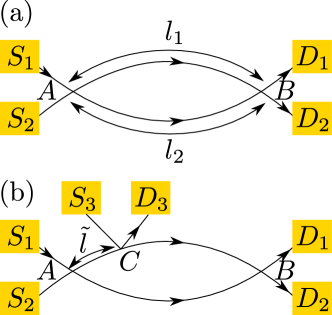
Figure 1: Illustration of the Mach-Zehnder interferometers (MZIs) under study. Chiral channels are represented by full lines leading from the sources ($S_{1}$ — biased and $S_{2}$ — grounded) to the drains ($D_{1}$ and $D_{2}$). Inter-edge tunneling takes place at intersection points. (a) A standard MZI with arms 1 and 2 of lengths $l_{1}$ and $l_{2}$, respectively. (b) The dangling end at $C$ (leading to $D_{3}$) serves as an absorber replacing the “lousy” bomb.

Here we analyze the correlations of transport through an e-MZI with a leaking edge. This is an electronic manifestation of a variant of the EV-bomb where the leaky-edge corresponds to an absorber instead of a bomb Mitchison and Massar (2001). In the particle-like limit of this device, the probability of a particle being absorbed and transmitted to the drains at the same time is zero. Such correlations in the case of many-particles will yield a non-vanishing result. This signifies the fact that the bomb may “explode” even if a signal is detected at the interferometer’s dark port. Employing a wave-like scattering matrix formulation, we compute the experimentally measurable many-body correlator and compare to two limiting cases (single particle impinging vs. a large influx of particles). Subsequently, we find the conditions for manifesting the wave-particle duality, and specifically obtaining the EV physics, in the context of many-body electronic system.

II System

We consider a standard e-MZI geometry where particles are injected from the source $S_{1}$ and eventually detected at the drains, $D_{1}$ and $D_{2}$ [see Fig. 1(a)]. Note that all channels are chiral, i.e. particles may move only in the direction of the arrow. The evolution of an injected wave packet through the setup is described by considering incoming scattering states from the various sources that are labeled by their quantum number $k$. Schematically, the state of a particle injected from $S_{1}$, after passing through beam-splitter $A$ at position $x=0$, is described by $\left|{i}\right>=r^{\phantom{\dagger}}_{A}\left|{1}\right>+t^{\phantom{\dagger}}_{A}\left|{2}\right>$, where $r^{\phantom{\dagger}}_{A}$ and $t^{\phantom{\dagger}}_{A}$ are the reflection and transmission amplitudes Not corresponding to beam-splitter $A$, and $\left|{1}\right>,\left|{2}\right>$ are the scattering states corresponding to the upper and lower e-MZI arms. Similarly, the beam splitter $B$ is characterized by reflection and transmission amplitudes $r_{B}$ and $t_{B}$, respectively. Between the beam splitters $A$ and $B$, orbital phases are accumulated along arm 1 and arm 2, i.e. $e^{ikl_{1}}$ and $e^{ikl_{2}}$, respectively. Additionally, for charged particles in the presence of a magnetic field, the relative phase of the two respective trajectories includes an Aharonov-Bohm phase $\Phi_{\rm AB}\equiv 2\pi\frac{\Phi}{\Phi_{0}}$, where $\Phi_{0}$ is a quantum of flux. With a proper gauge choice, we reabsorb these phases in an extra phase shift of the transmission coefficient of $t_{B}\to t_{B}e^{i\phi}$, with the interference phase $\phi=\phi^{\phantom{\dagger}}_{B}\equiv k(l_{2}-l_{1})+\Phi_{\rm AB}$.

We incorporate a semi-transparent absrober on the arm-1 of the e-MZI using an additional beam-splitter $C$ at position $0<\tilde{l}<l_{1}$ [see Fig.1(b)]. The propagation of an impinging particle is thus modified: the particle may exit the MZI through arm $3$ and reach drain $D_{3}$. The effect of this extra beam splitter evolves the scattering state component in arm-1, $\left|{1}\right>\to r^{\phantom{\dagger}}_{C}\left|{1}\right>+t^{\phantom{\dagger}}_{C}\left|{3}\right>$. This process is commonly referred to as partial-collapse and has been studied in the context of qubit-uncollapse Pryadko and Korotkov (2007); Katz et al. (2008) and null weak values Zilberberg et al. (2013, 2012, 2014).

This schematic evolution through the e-MZI can be conveniently recast in a scattering matrix formulation, i.e., we can write the state of a particle in the interferometer in second quantization, with an annihilation operator

$$\psi_{km}(x)=e^{ikx}\left\{\begin{array}[]{ll}a^{\phantom{\dagger}}_{km},&\hbox{$x<0;$}\\ b^{\phantom{\dagger}}_{km},&\hbox{$0<x<\tilde{l};$}\\ c^{\phantom{\dagger}}_{km},&\hbox{$\tilde{l}<x<l_{2};$}\\ d^{\phantom{\dagger}}_{km},&\hbox{$l_{m}<x.$}\\ \end{array}\right.$$ (5)

Here $m=1,2,3$ labels the different device arms and we assume arbitrarily that $l_{2}<l_{1}$. The operators $a_{km}$, $b_{km}$, $c_{km}$, $d_{km}$ are the annihilation operators of momentum eigenstates in the different sectors of the interferometer. They can be arranged in vectors $\mathbf{a}_{k}$, $\mathbf{b}_{k}$, $\mathbf{c}_{k}$, $\mathbf{d}_{k}$, labeled by the arm-index $m$, and are related by scattering matrices describing the effects of beam splitters via

$$\mathbf{b}^{\phantom{\dagger}}_{k}=\mathcal{S}^{\phantom{\dagger}}_{A}\mathbf{a}^{\phantom{\dagger}}_{k},\,\mathbf{c}^{\phantom{\dagger}}_{k}=\mathcal{S}^{\phantom{\dagger}}_{C}\mathbf{b}^{\phantom{\dagger}}_{k},\,\mathbf{d}^{\phantom{\dagger}}_{k}=\mathcal{S}^{\phantom{\dagger}}_{B}\mathbf{c}^{\phantom{\dagger}}_{k},$$ (6)

with

$$\mathcal{S}^{\phantom{\dagger}}_{i} =\left(\begin{array}[]{ccc}r^{\phantom{\dagger}}_{i}&t^{\phantom{\dagger}}_{i}&0\\ -t_{i}^{*}&r^{\phantom{\dagger}}_{i}&0\\ 0&0&1\end{array}\right)\,\,;\,\,i=A,B,$$ (10)

$$\mathcal{S}^{\phantom{\dagger}}_{C} =\left(\begin{array}[]{ccc}r^{\phantom{\dagger}}_{C}&0&-t^{\phantom{\dagger}}_{C}\\ 0&1&0\\ t^{\phantom{\dagger}}_{C}&0&r_{C}^{*}\end{array}\right).$$ (14)

III Single-particle limit

As a first step we analyze the the effect of the extra beam splitter $C$ using a schematic single-particle formulation. We assume that the incoming state is labeled by the quantum number $k$, which, for clarity we omit in the notation below. In the absence of the leakage port, the probability to measure the particle in drain $D_{1}$ is $P_{0}(i\rightarrow D_{1})=|\left<{D_{1}}\right|\left|{i}\right>|^{2}$, where $\left|{i}\right>=r^{\phantom{\dagger}}_{A}\left|{1}\right>+t^{\phantom{\dagger}}_{A}\left|{2}\right>$ includes the effect of beam splitter $A$, and we have defined $\left|{D_{1}}\right>=r^{\phantom{\dagger}}_{B}\left|{1}\right>+t^{\phantom{\dagger}}_{B}e^{i\phi}\left|{2}\right>$ to include the effect of beam splitter $B$ and the subsequent detection in $D_{1}$. We have used the subscript ${\cdot}_{0}$ to denote the probability in the absence of a leakage port. We obtain for the setup of Fig. 1(a), $P_{0}(i\rightarrow D_{1})=|r^{\phantom{\dagger}}_{A}|^{2}|r^{\phantom{\dagger}}_{B}|^{2}+|t^{\phantom{\dagger}}_{A}|^{2}|t^{\phantom{\dagger}}_{B}|^{2}+2|r^{\phantom{\dagger}}_{A}r^{\phantom{\dagger}}_{B}t^{\phantom{\dagger}}_{A}t^{\phantom{\dagger}}_{B}|\cos(\phi+\phi^{\phantom{\dagger}}_{T})$, where $\phi^{\phantom{\dagger}}_{T}=\arg(r^{\phantom{\dagger}}_{A}r^{\star}_{B}t^{\phantom{\dagger}}_{A}t^{\star}_{B})$. We think of the state of the propagating electron as a superposition of quibit states, $\left|{1}\right>$, $\left|{2}\right>$.

Introducing the beam-splitter $C$ on arm 1, allows the state $\left|{1}\right>$ to “leak out” (partial-collapse) to through branch 3 with probability $|t^{\phantom{\dagger}}_{C}|^{2}$ [cf. Fig. 1(b)]. The probability to reach drain $D_{3}$ is therefore,

$$P(i\rightarrow D_{3})=|r^{\phantom{\dagger}}_{A}|^{2}|t^{\phantom{\dagger}}_{C}|^{2}\,.$$ (15)

Upon detection of the injected electron in $D_{3}$, we declare the interference experiment void. In such a ”partial collapse” the state $\left|{1}\right>$ is projected out of the space spanned by $\left|{1}\right>$ and $\left|{2}\right>$. If such a projection-out does not take place (i.e. the electron is not detected in $D_{3}$), the original qubit state is rotated by the measurement’s back-action into $\left|{i_{C}}\right>=(1/\tilde{\mathcal{N}})\left(r^{\phantom{\dagger}}_{A}r^{\phantom{\dagger}}_{C}\left|{1}\right>+t^{\phantom{\dagger}}_{A}\left|{2}\right>\right)$ with normalization $\tilde{\mathcal{N}}=\sqrt{1-P(i\rightarrow D_{3})}$. Consequently, the probability for the particle to subsequently arrive in drain $D_{1}$ is $P(i_{C}\rightarrow D_{1})P(\overline{i\rightarrow D_{3}})$, where by overline we denote the complementary event, i.e. $P(\overline{i\rightarrow D_{3}})=1-P(i\rightarrow D_{3})$. Note that $P(i_{C}\rightarrow D_{1})$ can be written using the conditional probability $P(i\rightarrow D_{1}\,|\,\overline{i\rightarrow D_{3}})$. As a result we obtain that the particle would reach drain $D_{1}$ with the joint probability

$$P(i\rightarrow D_{1})=P(i\rightarrow D_{1},\overline{i\rightarrow D_{3}})=|r^{\phantom{\dagger}}_{A}|^{2}|r^{\phantom{\dagger}}_{B}|^{2}|r^{\phantom{\dagger}}_{C}|^{2}$$ (16)

$$+|t^{\phantom{\dagger}}_{A}|^{2}|t^{\phantom{\dagger}}_{B}|^{2}+2|r^{\phantom{\dagger}}_{C}||r^{\phantom{\dagger}}_{A}r^{\phantom{\dagger}}_{B}t^{\phantom{\dagger}}_{A}t^{\phantom{\dagger}}_{B}|\cos(\phi+\phi^{\phantom{\dagger}}_{T}+\phi^{\phantom{\dagger}}_{C})\,,$$

where $\phi^{\phantom{\dagger}}_{C}=\arg(r^{\phantom{\dagger}}_{C})$. Note that due to causality $P(i\rightarrow D_{1})=P(i\rightarrow D_{1},\overline{i\rightarrow D_{3}})$ and similarly

$$P(i\rightarrow D_{1},i\rightarrow D_{3})=0\,.$$ (17)

The fact that $P(i\rightarrow D_{1})\neq P_{0}(i\rightarrow D_{1})$ can be used to detect the presence of the leakage port. Specifically, if the MZI is tuned to have $P_{0}(i\rightarrow D_{1})=0$, the detection of a particle at $D_{1}$ in any single realization of the experiment indicates the presence of the leakage port without the particle having leaked out. If the particle is not detected at $D_{1}$, no conclusion on the presence of a leakage channel can be drawn. This is a manifestation of the EV-bomb detection scheme.

It is instructive to recover the results of this single particle analysis in the scattering matrix formalism, which provides the basis to analyze the statistical many-body effects in the following section. In the scattering matrix formalism we consider the injection of a single particle (in the scattering state $k$) into the system, i.e. $\left|{i_{k}}\right>=a^{\dagger}_{k,1}\left|{0}\right>$. The detection of the particle in $D_{1(3)}$ is described by the projection operator $\Pi_{D_{1}(D_{3})}\equiv d^{{\dagger}}_{k,1(3)}d^{\phantom{\dagger}}_{k,1(3)}$. From Eq. (6), the probabilities for the injected particle to reach $D_{1}$ or $D_{3}$ are

$$P(i_{k}\rightarrow D_{1})=\left<{0}\right|a^{\phantom{\dagger}}_{k,1}d^{{\dagger}}_{k,1}d^{\phantom{\dagger}}_{k,1}a^{\dagger}_{k,1}\left|{0}\right> =\mathcal{A}_{11},$$ (18)

$$P(i_{k}\rightarrow D_{3})=\left<{0}\right|a^{\phantom{\dagger}}_{k,1}d^{{\dagger}}_{k,3}d^{\phantom{\dagger}}_{k,3}a^{\dagger}_{k,1}\left|{0}\right> =\mathcal{B}_{11}\,,$$ (19)

where we have introduced the quantities $\mathcal{A}_{ij}\equiv(\mathcal{S}_{A}^{{\dagger}}\mathcal{S}_{B}^{{\dagger}}\mathcal{S}_{C}^{{\dagger}})_{i1}(\mathcal{S}_{C}\mathcal{S}_{B}\mathcal{S}_{A})_{1j}$, $\mathcal{B}_{ij}\equiv(\mathcal{S}_{A}^{{\dagger}}\mathcal{S}_{B}^{{\dagger}}\mathcal{S}_{C}^{{\dagger}})_{i3}(\mathcal{S}_{C}\mathcal{S}_{B}\mathcal{S}_{A})_{3j}$. Indeed, an explicit evaluation of $\mathcal{A}_{11}$ and $\mathcal{B}_{11}$ yields, for Eqs. (18) and (19) exactly the same expressions as Eqs. (16) and (15), respectively.

Additionally, the joint probability of detecting a particle at $D_{1}$ and $D_{3}$ is given by

$$P(i\rightarrow D_{1},i\rightarrow D_{3})\left<{0}\right|a^{\phantom{\dagger}}_{k,1}d^{{\dagger}}_{k,3}d^{\phantom{\dagger}}_{k,3}d^{{\dagger}}_{k,1}d^{\phantom{\dagger}}_{k,1}a^{\dagger}_{k,1}\left|{0}\right>\\ =\sum_{\beta=1}^{3}\mathcal{A}_{1\beta}\mathcal{B}_{\beta 1}\equiv 0\,,$$ (20)

where, when the incoming state is of a single particle, we recover the result in Eq. (17).

The results of this section describe experiments where a single particle is injected into the interferometer. While this is possible in quantum optics, it does not represent the typical experimental conditions of electronic devices. Single-particle sources have been only recently reported in some specifically designed experimental architectures Dubois et al. (2013). Since many-electron physics is an essential part of quantum reality, we next analyze this limit.

IV Many-body conditional correlations

In a typical experiment with e-MZI, particles are injected into the source from a voltage biased reservoir, and are collected in the drain over a macroscopically long time. This being the case, only statistical quantities averaged over a many-particle ensemble are accessible, and the signals at the detector correspond to statistical averages of the source-drain transition probabilities computed in the previous section. Specifically, for an e-MZI with a voltage bias $eV$ at $S_{1}$, the measured current at $D_{1}$ is given by the rate of electrons reaching this drain out of the total rate, $eV/\hbar$, of electrons impinging from the source. The currents through the device are therefore statistical probabilities for an impinging electron to reach the various drains, and are precisely given in terms of the probabilities calculated in the single-particle picture above: the current at drain $j$ will be given by $I_{j}=(e^{2}/h)P(i\rightarrow D_{j})V$. When the signal in $D_{1}$ is collected over a large number of particles, any outcome of the IFM-experiment would have a macroscopic leakage of particles in $D_{3}$ even if the e-MZI is tuned to have a vanishing current in the absence of the port $D_{3}$. Hence, in the original formulation of the problem with the bomb, the bomb would necessarily explode. In short, under the above conditions the detection of the current at $D_{3}$ does not constitute an uncontested manifestation of IFM.

Can, and under what conditions, an electronic MZI setup reproduce the original EV bomb measurement scheme? In order to clarify this we focus on the difference between the single-particle results and the many-particle statistical averages relevant for experiments, which appears when dealing with joint probabilities.

This is clearly demonstrated considering, e.g., the statistical joint probability of detecting particles at drain $D_{1}$ and $D_{3}$. In order to relate such a joint probability with a quantity directly accessible in experiments, we next study the current-current correlations in a many-body (albeit non-interacting) system. We assume that a voltage bias $V$ is applied to the source $S_{1}$, which is held at temperature $T$. For a system with linear dispersion relation, the current operator is $\hat{I}_{i}(x,t)=ev:\psi_{i}^{{\dagger}}(x,t)\psi_{i}(x,t):$, where $\psi_{i}(x,t)$ is the annihilation operator in the $i$-th arm, and the normal order operator, $:\,:$, indicates the subtraction of the mean equilibrium contribution.

We consider the cross-current correlation defined by

$$F_{1,3}\equiv\frac{h^{2}}{e^{4}V^{4}\tau}\int_{-\tau/2}^{\tau/2}dt\left\langle\hat{I}_{3}(x_{0},t)\hat{I}_{1}(x,0)\right\rangle,$$ (21)

where $\tau$ is an infrared cut-off, $\tau\gg\frac{L}{v}$, and $x_{0},x>l_{1}$. Importantly, since the average current is related to the electron transfer probability by the factor $e^{2}V/h$, the prefactor in the definition of $F_{1,3}$ allows us to directly compare this correlator with the averaged joint probability of detecting electrons at drain $D_{1}$ and $D_{3}$ [cf. Eq. (20)].

Using Wick’s theorem, the fact that all ohmic contacts are grounded apart from $S_{1}$ which is at $eV$, the identity $f_{\alpha}(1-f_{\beta})=\frac{1}{2}\left[f_{\alpha}(1-f_{\alpha})+f_{\beta}(1-f_{\beta})+(f_{\alpha}-f_{\beta})+(f_{\alpha}-f_{\beta})^{2}\right]$ where $f$ is the Fermi-Dirac distribution, and the limit of $\tau\gg L/v$, we obtain

$$F_{1,3}\equiv F_{\infty}(\alpha,\Delta\tilde{L})-F_{N}(\alpha,\Delta\tilde{L})=\frac{1}{\alpha}|r_{A}|^{2}|t_{C}|^{2}\Bigg{[}\alpha\left(|t_{A}|^{2}|t_{B}|^{2}+|r_{A}|^{2}|r_{B}|^{2}|r_{C}|^{2}\right)+2K(\alpha,\Delta\tilde{L})|t_{A}t_{B}r_{A}r_{B}r_{C}|\cos[\Phi(\alpha,\Delta\tilde{L},\Phi_{\rm AB})]\Bigg{]}$$

$$-\frac{1}{\alpha N}|r_{A}|^{2}|t_{C}|^{2}\Bigg{[}L(\alpha)\left(|t_{A}|^{2}|t_{B}|^{2}+|r_{A}|^{2}|r_{B}|^{2}|r_{C}|^{2}\right)+2M(\alpha,\Delta\tilde{L})|t_{A}t_{B}r_{A}r_{B}r_{C}|\cos[\Phi(\alpha,\Delta\tilde{L},\Phi_{\rm AB})]\Bigg{]}\,.$$ (22)

where $F_{\infty}$ and $F_{N}$ are functions of the dimensionless parameters $\alpha=eV\beta/(2\pi)$, $\Delta\tilde{L}=\pi(l_{2}-l_{1})/(\hbar\beta v)$, and $N=eV\tau/(2\pi\hbar)$. Here $\beta=1/(k_{B}T)$ is the inverse temperature. We have also introduced the functions $K(\alpha,\Delta\tilde{L})=\sin[\alpha\Delta\tilde{L}]/\sinh[\Delta\tilde{L}]$, $L(\alpha)=(\pi\alpha\coth[\pi\alpha]-1)/\pi$, $M(\alpha,\Delta\tilde{L})=(\pi\sin[\alpha\Delta L]\coth[\pi\alpha]-\Delta\tilde{L}\cos[\alpha\Delta\tilde{L}])/(\pi\sinh[\Delta L])$, and $\Phi(\alpha,\Delta\tilde{L},\Phi_{\rm AB})=\Phi_{\rm AB}+\phi^{\phantom{\dagger}}_{T}+\phi^{\phantom{\dagger}}_{C}+\alpha\Delta\tilde{L}$.

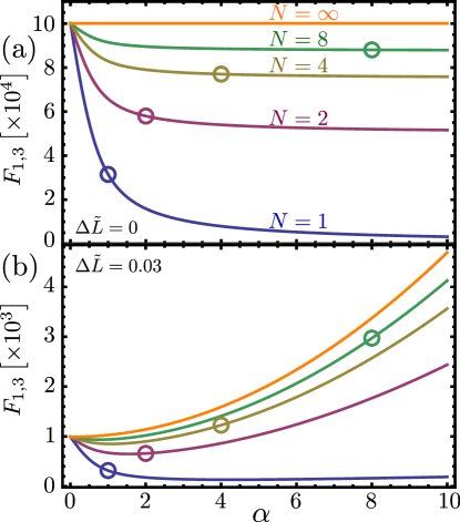
Figure 2: The many-body cross-current correlator as a function of $\alpha$ [cf. (22)]. Here, we have taken $|t_{C}|^{2}=0.3$,$|r_{A}|^{2}=|r_{B}|^{2}=0.5$ and $\Phi_{\rm AB}+\phi^{\dagger}_{T}+\phi^{\dagger}_{C}=\pi$. For a temperature of $T=10$mK the parameter $\alpha$ corresponds to realistic bias values of up to $\sim 54\mu$V. The different plots correspond to different values of $N=1\ldots 10$. As a function of $\alpha$ for a fixed $T$, $\tau$ should be changed in order to keep $N$ constant, i.e. $\tau=N\frac{2\pi\hbar}{eV}=N\frac{\hbar\beta}{\alpha}\sim 7.63823\times 10^{-10}(N/\alpha)$[second]. We mark by circles the point $\alpha\equiv N$ as the threshold for which our assumption $\tau\gg L/v$ breaks for existing electronic interferometers Neder et al. (2007). (a) The case of $\Delta\tilde{L}\rightarrow 0$. (b) The case of $\Delta\tilde{L}=0.03$ where dephasing affects both the classical and quantum correlators (due to varying interference lengths per wavenumber). Nonetheless, the single-particle limit remains unaffected as expected from Eq. (17).

Before discussing the implication of this result, it is instructive to contrast the many-body conditional correlator to purely classical correlations of an ensemble of statistically independent impinging electrons. In the latter case, we obtain the statistical average of a joint signal at port $D_{1}$ and $D_{3}$:

$$\tilde{P}(i\rightarrow D_{1},i\rightarrow D_{3})=P(i\rightarrow D_{1})P(i\rightarrow D_{3})\\ =|r^{\phantom{\dagger}}_{A}|^{2}|t^{\phantom{\dagger}}_{C}|^{2}\Big{[}|r^{\phantom{\dagger}}_{A}|^{2}|r^{\phantom{\dagger}}_{B}|^{2}|r^{\phantom{\dagger}}_{C}|^{2}+|t^{\phantom{\dagger}}_{A}|^{2}|t^{\phantom{\dagger}}_{B}|^{2}\\ +2|r^{\phantom{\dagger}}_{C}||r^{\phantom{\dagger}}_{A}r^{\phantom{\dagger}}_{B}t^{\phantom{\dagger}}_{A}t^{\phantom{\dagger}}_{B}|\cos(\phi+\phi^{\phantom{\dagger}}_{T}+\phi^{\phantom{\dagger}}_{C})\Big{]}\,.$$ (23)

For a better comparisson with the full many-body results that include the effect of averaging over a statistical ensamble due to termal fluctuations, as well as out-of equilibrium voltage bias, one can further average over a density matrix, $\rho$, that describes and ensemble of initial states. For example, assuming that a voltage bias $V$ is applied to the source $S_{1}$, which is held at temperature $T$, the state of the impinging electrons is described by $\rho=(1/L)\sum_{k}[f(\hbar vk-eV)-f(\hbar vk)]a_{k1}^{{\dagger}}a_{k1}$, where $f(x)$ is the Fermi-Dirac distribution, and the system length, $L$, is taken to be la largest length scale in the problem. When averaged over the initial density matrix, the “classical” correlations in Eq. (23) yield

$$\tilde{P}(i\rightarrow D_{1},i\rightarrow D_{3})=|r^{\phantom{\dagger}}_{A}|^{2}|t^{\phantom{\dagger}}_{C}|^{2}\left[|r^{\phantom{\dagger}}_{A}|^{2}|r^{\phantom{\dagger}}_{B}|^{2}|r^{\phantom{\dagger}}_{C}|^{2}+|t^{\phantom{\dagger}}_{A}|^{2}|t^{\phantom{\dagger}}_{B}|^{2}\right]\\ +2\frac{K(\alpha)}{\alpha}|r^{\phantom{\dagger}}_{C}||r^{\phantom{\dagger}}_{A}r^{\phantom{\dagger}}_{B}t^{\phantom{\dagger}}_{A}t^{\phantom{\dagger}}_{B}|\cos\left[\Phi(\alpha,\Delta\tilde{L},\Phi_{\rm AB})\right]\,.$$ (24)

Comparing the statistical probability analysis in Eq. (24) with the many-body joint correlation in Eq. (22), we obtain that $\tilde{P}(i\rightarrow D_{1},i\rightarrow D_{3})=F_{\infty}$, which is the dominant contribution of $F_{1,3}$ in the zero-frequency DC-limit. Indeed, this represents the well-known fact that $\lim_{\tau\to\infty}\int_{-\tau/2}^{\tau_{2}}dt\langle\hat{I}_{3}(x_{0},t)\hat{I}_{1}(x,0)\rangle=\langle\hat{I}_{3}(x_{0},t)\rangle\langle\hat{I}_{1}(x,0)\rangle\tau$. Similarly, a standard analysis of current-current correlations Blanter and Buttiker (2000) singles out the non-trivial correlations in the cross-current noise $S_{1,3}\equiv\lim_{\tau\to\infty}\int_{-\tau/2}^{\tau_{2}}dt(\langle\hat{I}_{3}(x_{0},t)\hat{I}_{1}(x,0)\rangle-\langle\hat{I}_{3}(x_{0},t)\rangle\langle\hat{I}_{1}(x,0)\rangle)$. These non-trivial contributions are encoded in the term $F_{N}=S_{1,3}/(\hat{I}_{0}^{2}\tau)$ of the many-body cross-current correlation in Eq. (22). Technically it corresponds to a particle-hole loop contribution.

While at low frequencies, $F_{\infty}$ is the dominant contribution to cross-current correlations, Eq. (22) clearly shows how, for measurements averaged over a finite time, the effects of $F_{\infty}$ and $F_{N}$ are competing. In fact, they become of the same order for short measurements times, such that the average currents are comparable with their fluctuations, i.e., $\langle\hat{I}_{3}(x_{0},t)\rangle\langle\hat{I}_{1}(x,0)\rangle\tau\sim S_{1,3}$. In particular, one expects that in the limit where the average number of particles in the interferometer is $\sim 1$ during the measurement time $\tau$, these two terms cancel each other, and we can recover the single-particle result of Eq. (17). By estimating the average number of electrons impinging on the e-MZI during the measurement time by $N=\frac{eV\tau}{2\pi\hbar}$, we are in the position of interpreting the cross-current correlator in terms of a crossover between single-particle quantum-mechanical correlations and classical statistical correlations.

Fig. 2(a) depicts the cross-current correlations as function of the voltage bias, $\alpha$, measured in units of temperature, for different values of $N$. For any value of $N$, at $\alpha\lesssim 4$, thermal fluctuations dominate over the quantum ones, and the correlations will ultimately reduce to those of classical waves. For large $\alpha$, upon decreasing $N$, $F_{1,3}$ decreases, and for $N\sim 1$ it is essentially vanishing, i.e., we obtain $F_{1,3}\ll F_{\infty}$ which signals that quantum correlations are important. Note that Eq. (22), depicted in Fig. 2, is valid for $\tau\gg L/v$. Recall that as a function of $\alpha$ for a fixed temperature $T$, $\tau$ changes in order to keep a constant $N$, i.e. $\tau=N\frac{2\pi\hbar}{eV}=N\frac{\hbar\beta}{\alpha}\sim 7.63823\times 10^{-10}(N/\alpha)$[second], where we considered $T=10$mK. Taking experimental values of existing electronic interferometers, $L\sim 10\mu$m and $v\sim 2-6\times 10^{-4}$m/s Neder et al. (2007), we mark the point $\alpha\equiv N$ as a threshold beyond which our prediction no longer holds. As such, in order to reach the limit of single-particle demonstration of IFM, one should construct smaller interferometers or generate higher edge mobility. Alternatively, one could consider single-particle injection on top of a Fermi sea Dubois et al. (2013), but this is beyond the scope of our analysis.

In Fig. 2(b), we see the effect of a finite $\Delta\tilde{L}$. As each wavenumber experiences a slightly different interference path, both the classical and quantum many-body correlations are affected by averaging over many wavenumbers. As a result, when many particles are considered [Eq. (22)] the result moves further away from the single-particle limit of Eq. (17) reflecting this effective dephasing. Nonetheless, in the limit of short pulses, $N=1$, the correlator yields an outcome that agrees with the single-particle picture.

V Conclusions

The main focus of this study is the assessment of feasible detection of IFM in a genuine many-body electronic system. To this goal, we have analyzed an electronic MZI with a leakage port located on one of the interferometer arms, which servs as an experimentally viable implementation of the EV-bomb gedanken experiment. We considered the typical experimental settings when an ensemble of particles is injected in the interferometer, i.e., the current in the interferometer yields a statistically averaged signal. We analyzed the cross-current correlation at the dark and leakage ports, which is vanishing in the single-particle original proposal of the experiment, but remains generally finite in the many-particle statistical implementation. This has allowed us to identify the parameters’ regime (voltage bias, temperature) for which the many-body correlations approach the single-particle result. We find the regime where the wave-particle duality emerges is lies just at the frontiers of actual experiments with electronic MZIs, where the main limitations are due to the size of the interferometer and the mobility of the electrons at the edges of a Hall bar.

In summary, our results show that the detection of IFM in a many-body electronic system seems to involve two competing facets that need to be dealt with: IFM a-la Elitsur-Vaidman requires to deal with particles (that, in principle, can be pin-pointed to a specific spatial coordinate); at the same time, the setup employed is an interferometer, which invokes the wave character of the quantum object. One thus needs to fine-tune the system to zoom on a regime where particle-wave duality is manifest. Our analysis might trigger experiments with single-electron biased MZIs, where this physics may be elucidated.