On the non-thermal $\kappa$-distributed electrons in planetary nebulae and H II regions: the $\kappa$ index and its correlations with other nebular properties

Abstract

Recently, a suspicion arose that the free electrons in planetary nebulae (PNe) and H II regions might have non-thermal energy distributions. In this scenario, a $\kappa$ index is introduced to characterize the electron energy distributions, with smaller $\kappa$ values indicating larger deviations from Maxwell-Boltzmann distributions. Assuming that this is the case, we determine the $\kappa$ values for a sample of PNe and H II regions by comparing the intensities of [O III] collisionally excited lines and the hydrogen Balmer jump. We find the average $\kappa$ indices of PNe and H II regions to be 27 and 32, respectively. Correlations between the resultant $\kappa$ values and various physical properties of the nebulae are examined to explore the potential origin of non-thermal electrons in photoionized gaseous nebulae. However, no positive result is obtained. Thus the current analysis does not lend to support to the idea that $\kappa$-distributed electrons are present in PNe and H II regions.

1 Introduction

The accurate determination of element abundance in planetary nebulae (PNe) and H II regions is important for understanding the matter cycle between stars and the ISM. This crucially depends on the assumed free electron energy distributions (EEDs) in that the emissivities of recombination lines (RLs) and collisionally excited lines (CELs) are given by the integral of the known energy dependence of the relevant atomic cross section over the EEDs. In the past, the generally accepted assumption is that free electrons in photoionized nebulae are in thermal equilibrium, in which the EEDs follow a Maxwell-Boltzmann (MB) distribution, characterized by a single parameter, the electron temperature. However, this assumption has never been validated by direct observations, but is largely based on the theoretical argument that the electron thermalization time-scale via elastic collisions is much shorter than the other known processes that produce non-thermal electrons under typical nebular conditions. Although there were some early debates about the MB distributions in PNe (see Introduction of Storey & Sochi, 2014), it has not been seriously doubted until recently.

It has been long known that there exist non-MB distributed particles in solar and space plasmas (e.g. Vasyliunas, 1968; Feldman et al., 1975; Seely et al., 1987; Cranmer, 2014). The $\kappa$ distributions, consisting of a low-energy MB core and a high-energy power law tail, are introduced to characterize those non-MB distributions, with smaller $\kappa$ indices indicating larger deviations from MB distributions. Leubner (2002) and Livadiotis & McComas (2009) show that the $\kappa$ distributions can arise naturally from Tsallis’ nonextensive statistical mechanics. In non-isolated systems, on-going accelerations, such as those induced by magnetic reconnections, shocks, and turbulence, can generate non-thermal electrons, which are predicted to have $\kappa$ EEDs according to the non-equilibrium generalization of the MB distributions. This raises a critical question of whether the $\kappa$ distributions also widely exist in other astronomical environments other than the solar system plasmas, such as photoionized gaseous nebulae, and the MB distributions are only a special case of equilibrium.

Inspired by the studies of solar system plasmas, Nicholls et al. (2012, 2013) proposed that the $\kappa$ distributions provide a potential solution for the long-standing problem in nebular physics, viz., the discrepancies of electron temperatures and heavy-element abundances derived from RLs and CELs. The RL/CEL discrepancy is commonly quantified by the ratio of O²⁺ abundances obtained from RLs and CELs, called abundance discrepancy factor (ADF; Liu, 2006). The ADFs range from 1 to 71, with the most extreme case found in the PN Hf 2-2 (Liu et al., 2006). As the high-energy tail of $\kappa$ EEDs preferably contribute to the emission of CELs relative to RLs, CEL diagnostics will result in an overestimated electron temperature, leading to underestimated element abundances, when ones use MB distributions to interpret the spectra actually produced by $\kappa$ distributions. Later on, $\kappa$ distributions were invoked to explain the abundance discrepancies in H II regions derived from strong-line and $T_{\rm e}$-based methods (Dopita et al., 2013), and the abnormal C II line ratios in Type 2 quasars (Humphrey & Binette, 2014). The $\kappa$ indices represent an additional free parameter to match model to observations. In order to examine the validation of this solution, it is important to develop methods to diagnose the EEDs in photoionized gaseous nebulae.

The first attempt to discriminate EEDs in PNe was made by Storey & Sochi (2013), who investigated the intensities of C II dielectronic recombination lines under $\kappa$ and MB distributions and compared the theoretical predictions with the spectra of a few PNe. However, taking into account the uncertainties, it is hard to distinguish the two scenarios from the limited observations. Therefore, they cannot draw any definite conclusion.

Another approach to sample the EEDs in PNe is to simulate the H I free-bound (FB) emission (Zhang et al., 2014, hereafter ZLZ), i.e. the nebular optical continua. Using that method, ZLZ found that the observed H I FB spectra of four PNe with extremely large ADFs cannot be interpreted in terms of a single MB EED, but are equally well fitted by either a two-component MB model or by $\kappa$-distributed electrons. However, shortly thereafter, a similar study independently undertook by Storey & Sochi (2014, hereafter SS) shows that the two-component MB model actually better accounts for the H I FB spectrum of Hf 2-2 than $\kappa$-distributed electrons, in contrast to ZLZ’s conclusion. Storey & Sochi (2015a) attributed the discrepancy to the different treatments of H11 emission coefficient, $\alpha_{\rm eff}$(H11). In both models of ZLZ and SS, the continuum intensity has been normalized to the integrated intensity of the H11 Balmer line at 3770 Å. Following Nicholls et al. (2012), ZLZ used an approximate function to obtain $\alpha_{\rm eff}$(H11) for a $\kappa$ distribution. The approximation is generally sufficiently accurate, but at high temperatures and/or extremely low $\kappa$ indices a correction factor should be considered (see Table 1 of SS). At the typical nebular temperature of $10^{4}$ K, the correction increases rapidly from 2 to 30 percent as the $\kappa$ index decreases from 10 to 2. However, we do not think that this is the main reason causing the inconsistent results between ZLZ and SS. In the first place, it seems unlikely (although not impossible) that the spectrum fitting based on $\kappa$ distribution can be greatly improved by using a more inaccurate $\alpha_{\rm eff}$(H11). Moreover, the model fitting largely relies on the slope of H I FB continuum, and the approximate treatment of H11 only results in an uncertain scaling constant and thus only has minor effect on the result. We note that the primary difference between the modelling approaches of ZLZ and SS is in the treatment of subtraction of the underlying stellar light contaimination. The spectral energy distribution of contaminating stellar continuum has been assumed to follow a power-law, $I_{\lambda,\rm star}\sim\lambda^{-\beta}$. SS obtained $I_{\lambda,\rm star}$ by fitting the model continuum to the observed one in two wavelength segments longer than the Balmer edge (3780–3790 and 4180–4230 Å). For this purpose, they need to presuppose a H I FB continuum for a given temperature and $\kappa$ value. In contrast, ZLZ considered the whole line-free spectral range 3550–4200 Å, and optimized the model fitting by adjusting the ${\beta}$ value. The latter may provide a more flexible way to fit the global spectral behavior. It seems to us this different treatment of the underlying stellar light contamination might actually be the primary cause for the different conclusions drawn by SS and ZLZ. We should point out that accurate subtraction of background contribution and reliable continuum flux calibration are the main challenge of using H I FB continuum to probe the EEDs.

Although no solid observational evidence is found to support the idea of deviation from MB EEDs in nebulae, if the $\kappa$ distributions were proven valid, one would need a new paradigm for the study of nebular astrophysics. In this paper, we present determinations of the $\kappa$ indices for a sample of PNe and H II regions under the assumption that the $\kappa$ EEDs are fully responsible for the RL/CEL discrepancy problem. The reported $\kappa$ values could serve as a basis for future studies of this problem. The rest of the paper is organized as follows. In Section 2 we describe the methodology to derive the $\kappa$ indices from nebular spectra. The results are reported in Section 3. In Section 4 we explore the correlations of the resultant $\kappa$ values and other nebular properties, in order to investigate the potential causes of $\kappa$ EEDs. A summary is given in Section 5.

2 METHODOLOGY

2.1 The $\kappa$ distribution and its effects on plasma diagnostics

As quoted, the calculations of RL and CEL intensities largely depend on EEDs. The EED is quantified by $f(E)$, the fraction of electrons having an energy of $E$. In an equilibrium state, $f(E)$ is given by the MB function

$$f_{\rm MB}(E)=2\sqrt{\frac{E}{\pi}}\left(\frac{1}{k_{B}T_{\rm e}}\right)^{3/2}\exp\left(\frac{-E}{k_{B}T_{\rm e}}\right),$$ (1)

where $k_{B}$ is the Boltzmann constant, and $T_{\rm e}$ is the electron temperature. When the plasma is in a non-equilibrium stationary state, the EED follows a $\kappa$ distribution defined by

$$f_{\kappa}(E)=2\sqrt{\frac{E}{\pi}}\left(\frac{1}{k_{B}T_{U}}\right)^{3/2}\frac{\Gamma(\kappa+1)}{(\kappa-3/2)^{3/2}\Gamma(\kappa-1/2)}\left[1+\frac{E}{(\kappa-3/2)k_{B}T_{U}}\right]^{-\kappa-1},$$ (2)

where $\Gamma$ is the gamma function, $\kappa$ is a parameter $>1.5$ describing the degree of departure from the MB distribution, and $T_{\rm U}$ is the non-equilibrium temperature characterizing the mean kinetic energy. Lower $\kappa$ values represent larger departures from the MB distribution. As the $\kappa$ index approaches infinity, the $\kappa$ distribution decays to the MB distribution, where we have $f_{\kappa}(E)=f_{\rm MB}(E)$ and $T_{\rm U}=T_{\rm e}$.

Compared to the MB distribution, the $\kappa$ distribution has a high-energy tail that is power-law distributed. For a given $T_{\rm U}$ value, the fraction of high-energy electrons increases with decreasing $\kappa$. The low-energy parts of a $\kappa$ distribution can be approximated by a MB distribution of a temperature $T_{\rm core}=(1-1.5/\kappa)T_{\rm U}$. Since $\int f_{\kappa}(E)dE\equiv f_{\rm MB}(E)dE\equiv 1$, this MB function should be scaled by a factor of $R<1$ to match the core of the $\kappa$ distribution, where $R$ can be obtained by requiring $Rf_{\rm MB}(k_{B}T_{\rm core})=f_{\kappa}(k_{B}T_{\rm U})$. From Equations (1) and (2), we have

$$R=2.718\frac{\Gamma(\kappa+1)}{\kappa^{3/2}\Gamma(\kappa-1/2)}\left(1+\frac{1}{\kappa}\right)^{-\kappa-1}.$$ (3)

The $(1-R)$ value represents the fraction of non-thermal electrons, which ranges from 0.01 to 0.45 when the $\kappa$ index decreases from 100 to 2.

It is conceivable that incorrect results will be obtained if ones utilize the MB-based method to determine the electron density ($N_{\rm e}$) and $T_{\rm e}$ of the plasma with the $\kappa$ EED. If the $N_{\rm e}$-diagnostic lines are dominantly excited by low-energy electrons (e.g. RLs and infrared fine-structure CELs), the MB-based method will result in a $N_{\rm e}$ value that is overestimated by a factor of $1/R$. The Balmer jump (BJ) of H I recombination spectrum and the [O III] nebular and auroral lines are the most used $T_{\rm e}$-diagnostics in nebulae. The former is mostly contributed by low-energy electrons, and thus mainly measures the low-temperature MB core, while the latter arises from collisional excitation of high-energy electrons. It follows that ones may obtain a lower $T_{\rm e}$(BJ) relative to $T_{\rm e}$([O III]) under the traditional assumption of MB EEDs.

2.2 Determination of $\kappa$ indices

The $\kappa$ and $T_{\rm U}$ values of an isotropic plasma can be derived by comparing the BJ intensity, $J_{\rm B}=[I(\lambda 3650^{-})-I(\lambda 3650^{+})]/I({\rm H11})$ Å^-1, and the nebular-to-auroral line ratio of [O III], $R$([O III])$=$[O III]$\lambda\lambda(4959+5007)/4363$. Zhang et al. (2004) have simulated the H I FB spectrum with MB EEDs. A similar method can be used to calculate the BJ with $\kappa$ EEDs, in which $f_{\kappa}(E)$ was substituted for $f_{\rm MB}(E)$. The dependence of the BJ intensity on $\kappa$ and $T_{\rm U}$ has been elucidated in ZLZ. At a particular $T_{\rm U}$ value, a lower $\kappa$ index leads to a higher $J_{\rm B}$. We use the same approach as in ZLZ to simulate the BJ intensity. In order to normalize $J_{\rm B}$, we take the effective recombination coefficients of H11 under $\kappa$ EEDs, $\alpha^{\rm eff}_{\kappa}$(H11), recently tabulated by Storey & Sochi (2015a). For either recombination or collision processes, the rate coefficient is given by

$$\alpha_{\kappa}=\int\sigma(E)\sqrt{\frac{2E}{m_{\rm e}}}f_{\kappa}(E)dE,$$ (4)

where $m_{\rm e}$ is the electron mass, and $\sigma(E)$ is the relevant cross-section. In order to simulate the H I FB transition, the recombination cross-section, $\sigma(E)$, is determined from the photoionization cross-section through the Milne relation. Then $\alpha^{\rm eff}_{\kappa}$(H11) can be deduced by solving the collisional-radiative recombination problem. Storey & Sochi (2015a) performed such calculations, and derived the $\alpha^{\rm eff}_{\kappa}$(H11) values at various combinations of $\kappa$, temperature, and density. The dependence of $R$([O III]) on $\kappa$ and $T_{\rm U}$ can be obtained by solving the level populations for the five-level atomic model, for which we require the effective collision strengths with $\kappa$ EEDs. In principle, the effective collision strengths can be determined from Equation (4) if we have the collisional cross-section, $\sigma(E)$. However, the cross sections are difficult to be tabulated and are not always available in literature. Recently, Storey & Sochi (2015b) calculated the $\kappa$-dependent effective collision strengths for electron collision excitation of the [O III] CELs. We have taken their reported data for the calculations of $R$([O III]). Since the non-thermal electrons would strengthen the auroral lines more than the nebular lines, the $R$([O III]) value decreases with decreasing $\kappa$ values.

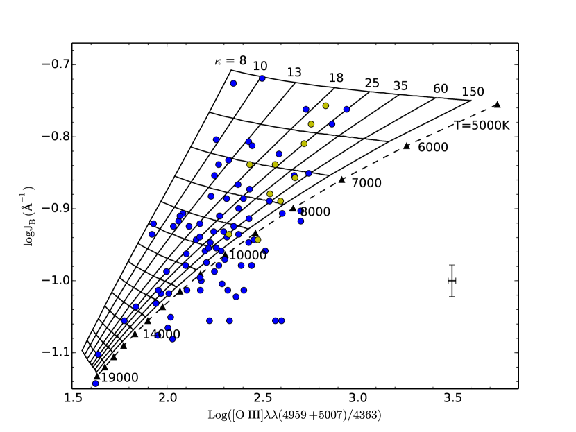
Figure 1: The intensities of the Balmer Jump versus the [O III] line ratios as functions of $\kappa$ and $T_{\rm U}$. The dashed curve with filled triangles shows the theoretical predictions from MB electron distributions at different temperatures. The filled circles represent the observations of PNe (blue) and H II regions (yellow). A typical error bar is shown in the lower right corner.

Figure 1 plots the theoretical predictions of $J_{\rm B}$ versus $R$([O III]) as functions of $\kappa$ and $T_{\rm U}$, as well as those of MB EEDs. The calculations are essentially independent of $N_{\rm e}$ because the critical densities for the involved lines are much larger than the typical nebular density. Therefore, we have assumed a constant $N_{\rm e}$ of 10³ cm^-3 for all the calculations. An inspection of Figure 1 shows that $J_{\rm B}$ and $R$([O III]) are more sensitive to the $\kappa$ index at low temperature. With increasing $T_{\rm U}$, the peak of EEDs shift towards higher energy, and thus more electrons with energy lying within the MB core can contribute to the excitation of [O III] CELs. As a result, the $J_{\rm B}$ versus $R$([O III]) relations would converge to that of MB EEDs at higher temperature. As shown in Figure 1, the $\kappa$ index can be determined with a reasonable degree of accuracy from the observed $J_{\rm B}$ and $R$([O III]) in the regions of $\kappa<60$ and $T_{\rm U}<15000$ K.

The basic idea of this method is similar to that of Nicholls et al. (2012) through comparing $T_{\rm e}$(BJ) and $T_{\rm e}$([O III]). But the approach of Nicholls et al. (2012) contains some approximations, e.g., the rate coefficients are approximately obtained (see Section 1 and the discussion in SS), and they have assumed $T_{\rm e}({\rm BJ})=T_{\rm core}$. These approximations are generally justified, but would lead to larger uncertainties for low $\kappa$ index. In contrast, we have used the most recently reported atomic data, and thus are able to provide a more robust estimate of the $\kappa$ index.

Based upon the $T_{\rm e}$(BJ) versus $T_{\rm e}$([O III]) diagrams, Nicholls et al. (2012) concluded that PNe and H II regions have typical $\kappa$ indices of larger than 10. However, they did not present the $\kappa$ values for individual nebulae. In the present work we attempt to determine the $\kappa$ indices for a sample of gaseous nebulae, including 82 PNe and 10 H II regions. The data utilized were taken from work recently published by our research group and others (see Tables On the non-thermal $\kappa$-distributed electrons in planetary nebulae and H II regions: the $\kappa$ index and its correlations with other nebular properties & On the non-thermal $\kappa$-distributed electrons in planetary nebulae and H II regions: the $\kappa$ index and its correlations with other nebular properties). These high signal-to-noise spectra have been obtained with the purpose of investigating the RL/CEL discrepancy problem. With careful flux calibrations and dereddening corrections as well as accurate measurements of the Balmer Jump, they are particularly well suited for our analysis. In some cases, where the $J_{\rm B}$ values are not explicitly given in the literature, we deduced the $J_{\rm B}$ values through the $T_{\rm e}$(BJ) versus $J_{\rm B}$ relation of Liu et al. (2001, see their Equation (3)).

3 RESULTS

The observed $J_{\rm B}$ and $R$([O III]) values are overplotted in Figure 1. As the data are taken from different references, the measurement uncertainties are not available for all the observed values. We roughly estimate a typical error bar from our spectra, as shown in the lower right corner of this figure. The [O III] CELs are relatively strong, and thus $R$([O III]) can be obtained with high accuracy. The uncertainty of the $\kappa$ index mainly comes from the measurement of the Balmer Jump, and it steeply increases with increasing $\kappa$ and $T_{\rm U}$. If the EEDs follow single MB distributions, all the plotted points should lie on the dashed curve in Figure 1. However, most of them fall on the upper left of that curve, which can be explained in terms of $\kappa$ EEDs. There are a very small number of data points lying on the far lower right of the dashed curve, e.g. the regions of $T_{\rm e}({\rm BJ})>T_{\rm e}$([O III]). We can tentatively attribute this to shock heating in the outer low-ionized regions and/or the possible existence of metal-poor clumps, although the exact reason remains unclear.

The resultant $\kappa$ and $T_{\rm U}$, along with the other nebular properties, are given in Tables On the non-thermal $\kappa$-distributed electrons in planetary nebulae and H II regions: the $\kappa$ index and its correlations with other nebular properties & On the non-thermal $\kappa$-distributed electrons in planetary nebulae and H II regions: the $\kappa$ index and its correlations with other nebular properties for PNe and H II regions, respectively. In these tables, $N_{\rm e}$ is the average value of electron densities obtained by various $N_{\rm e}$-diagnostics available in the literature, and the effective density under $\kappa$ EEDs, $N_{\rm eff}$, is obtained through multiplying $N_{\rm e}$ by a factor of $R$ (see Section 2.1). In Figure 1, some data points are too close to the MB predictions to allow reliable determinations of $\kappa$, and we can only estimate a lower limit of 60. Excluding those with $\kappa>60$, we finally give the $\kappa$ indices of 47 PNe and 8 H II regions. The errors of $\kappa$ can be inferred graphically from Figure 1. It should be cautious in using the resultant values in the high-$\kappa$ and/or high-$T_{\rm U}$ regions for further analysis. As is clear in Figure 1, PNe distribute in more scattering and higher temperature regions than H II regions in the ($\kappa$, $T_{\rm U}$) parameter space. We obtain the average values of $\kappa=27$ and $32$ for the 47 PNe and 8 H II regions, respectively, suggesting that PNe probably have a systematically greater departure from MB EEDs than H II regions. We did not find very extreme PNe with $\kappa<8$. The average $\kappa$ index in nebulae is far larger than those in most of the other space plasmas (see Table 1 of Livadiotis, 2015), but is close to that of the low solar corona (10–25; Cranmer, 2014).

Tables On the non-thermal $\kappa$-distributed electrons in planetary nebulae and H II regions: the $\kappa$ index and its correlations with other nebular properties & On the non-thermal $\kappa$-distributed electrons in planetary nebulae and H II regions: the $\kappa$ index and its correlations with other nebular properties also list $T_{\rm e}({\rm BJ})$ and $T_{\rm e}([{\rm O~{}III}])$ reported in the literature. As quoted, $T_{\rm e}({\rm BJ})$ and $T_{\rm e}([{\rm O~{}III}])$ are respectively determined from $J$(BJ) and $R$([O III]) under the assumption of MB EEDs. In the scenario of $\kappa$ EEDs, the two parameters retrieved from $J$(BJ) and $R$([O III]) are substituted with $\kappa$ and $T_{\rm U}$. Namely, a consistent temperature $T_{\rm U}$ can be obtained through adjusting the $\kappa$ index. Therefore, $T_{\rm U}$ should be a value between $T_{\rm e}({\rm BJ})$ and $T_{\rm e}([{\rm O~{}III}])$, as confirmed in those tables. Since the $\kappa$ index is introduced for the purpose of interpreting the temperature discrepancy, $\delta t=T_{\rm e}([{\rm O~{}III}])-T_{\rm e}({\rm BJ})$, it is expected to be negatively correlated with $\delta t$. Such a correlation can be seen in Figure 2. The $\kappa$ index can be fitted to the expression

$$\kappa=1.5\exp\left(\frac{3.57}{\delta t^{0.42}}\right),$$ (5)

where $\delta t$ is in the unit of $10^{-3}$ K. Equation (5) can be used to conveniently determine the $\kappa$ index from the previously reported $T_{\rm e}({\rm BJ})$ and $T_{\rm e}([{\rm O~{}III}])$. Figure 2 also shows the histograms of $\kappa$ and $\delta t$, where PNe clearly exhibit an extended tail towards low $\kappa$ and high $\delta t$, and there is no H II region showing $\kappa<17$.

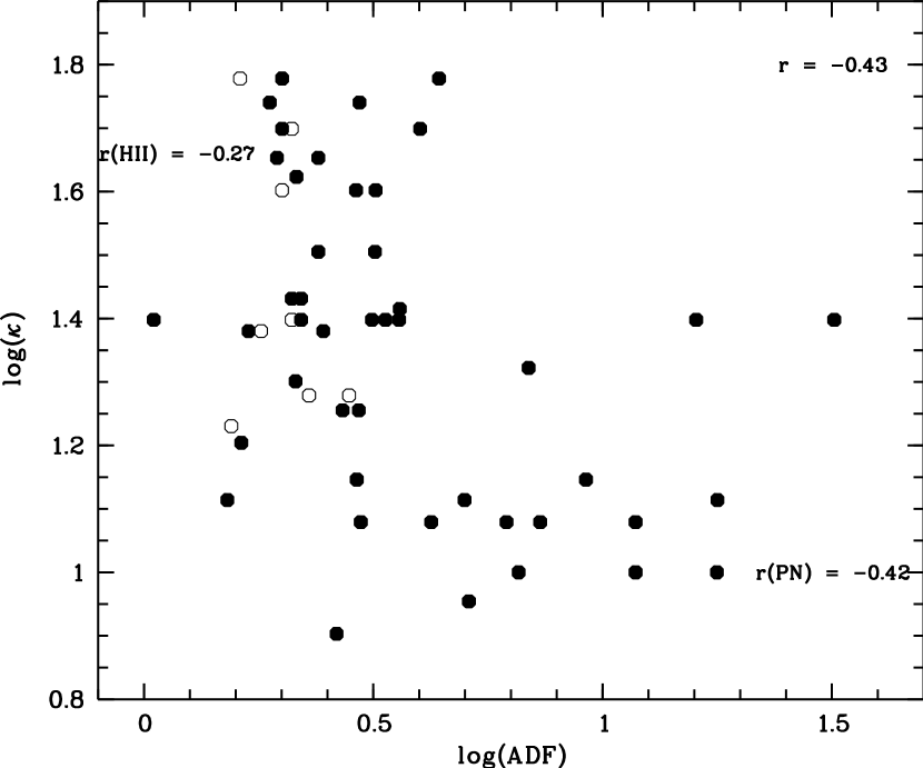
Figure 3: $\log\kappa$ versus $\log({\rm ADF})$ for PNe (filled circles) and H II regions (open circles) with corresponding correlation coefficients indicated. The correlation coefficient for the combined data is given in the upper right corner.

It has been well established that the RL/CEL temperature and abundance discrepancies are two relevant problems. A positive correlation between ADFs and $\delta t$ has been found in a small sample of PNe by Liu et al. (2001), suggesting that the two discrepancies are probably caused by a common underlying physical mechanism. If this is the case, we would expect that there exists a negative correlation between $\kappa$ and ADFs. Figure 3 plots $\kappa$ against ADFs, in which we indeed observe a loose negative correlation for our PN sample. The relationship between $\log(\kappa)$ and $\log$(ADF) is clearly non-linear, but similar to that between $\log(\kappa)$ and $\delta t$ (Figure 2), shows a ‘L’-shape in Figure 3. This is in agreement with Liu et al. (2001) who found a strong linear correlation between $\delta t$ and $\log$(ADF). For H II regions, however, the correlation coefficient is too low to be meaningful.

4 DISCUSSION

The $\kappa$ distribution provides a potential solution for the RL/CEL discrepancy problem, as illustrated in Figure 1. Using Equation (3), our results show that about $3.2\%$ and $2.7\%$ electrons are non-thermal in PNe and H II regions, respectively, suggesting that only minority of non-thermal electrons are able to account for the $T_{\rm e}$(BJ)/$T_{\rm e}$([O III]) discrepancy. Nicholls et al. (2012, 2013) discussed the possible formation of $\kappa$ EEDs in gaseous nebulae. Because the thermalization timescale of free electrons is proportional to the cube of the velocity, high-energy electrons may approach to equilibration state slower than their injection. Therefore, if energetic electrons could be continually and quickly injected, the $\kappa$ distribution would be developed. A key question is what the mechanism continually pumping and maintaining stable $\kappa$ EEDs could be in PNe and H II regions. The possibilities presented by Nicholls et al. (2012, 2013) include magnetic reconnections, local shocks, photoionization of dust, and X-ray ionization. The $\kappa$ indices determined in the present paper provide a useful foundation for investigating the postulated generation of non-thermal electrons. For that purpose, in this section we examine the correlations between $\kappa$ indices and other nebular properties.

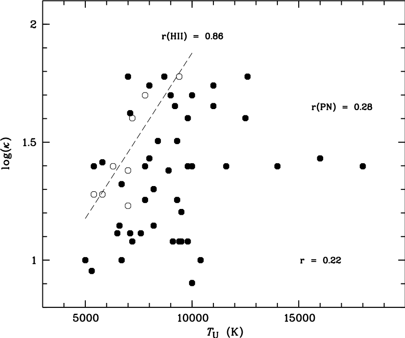
Figure 4: $\log\kappa$ versus $T_{\rm U}$ for PNe (filled circles) and H II regions (open circles). The dashed line is the best linear fit for H II regions. The correlation coefficients for PNe, H II regions, and the combined data are given.

Figure 4 shows that there is no apparent linear correlation between $\kappa$ and $T_{\rm U}$ for PNe. For cooler nebulae, a more significant fraction of electrons lying in the power-law high-energy tail contributes to the excitation of [O III] CELs in that the MB core is confined within a lower-energy region and thus has less contribution to the collisional excitation. This points to a positive correlation between $\kappa$ and $T_{\rm U}$. However, the situation is complicated by the fact that the suprathermal heating caused by energetic stellar winds can increase the kinetic temperature and decrease the $\kappa$ index, as suggested by Nicholls et al. (2012). A visual examination of Figure 4 seems to reveal that the $\kappa$ index roughly increases with increasing $T_{\rm U}$, but significantly decreases at the highest temperature. Although this behavior can be explained in terms of $\kappa$ EEDs, it cannot be viewed as a solid support for the $\kappa$ distribution. Figure 4 also suggests a stronger positive correlation for H II regions than PNe. A natural question to ask is whether the cause of RL/CEL discrepancies in H II regions differs from that in PNe. We require a larger sample and more sophisticated study to ascertain this.

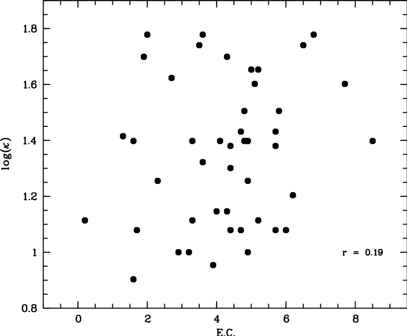
Figure 5: $\log\kappa$ versus E.C. for PNe. The correlation coefficient is indicated.

In Figure 5 we plot $\kappa$ against the excitation class (EC) of PNe. The excitation class can be determined from spectral line ratios, and is closely related to the effective temperature of the central stars. We calculated the ECs of PNe following the formalism suggested by Dopita & Meatheringham (1990), as tabulated in Table On the non-thermal $\kappa$-distributed electrons in planetary nebulae and H II regions: the $\kappa$ index and its correlations with other nebular properties. Although the classification scheme was developed for the Magellanic Cloud PNe, it should be able to serve as a measurement of the relative excitation conditions in Galactic PNe. Figure 5 demonstrates that no correlation exists between $\kappa$ and EC. We therefore do not find a trend that more pronounced departure from MB EEDs corresponds to harder radiation fields. Consequently, we cannot give any empirical evidence for the photoionzation by the radiation from central stars as the cause of non-thermal electron production.

Is it possible that the non-thermal electrons are generated by the kinetic energy released by the mass loss? NGC 40 and NGC 1501 are two PNe with Wolf-Rayet type central stars that are characterized by fast stellar winds and high mass-loss rates. We only discover moderate $\kappa$ indices for the two PNe, while those with the lowest $\kappa$ indices are not Wolf-Rayet PNe. Furthermore, García-Rojas et al. (2013) investigated the abundances of a sample of PNe with [WC]-type nucleus, and found that there is no discernible relation between the [WC] nature and the ADFs. Therefore, we can conclusively rule out the possibility that stellar winds are the main source producing non-thermal electrons.

We also examine the $\kappa$ indices by classifying the PNe according to their morphologies and Peimbert types (see the 10th column of Table On the non-thermal $\kappa$-distributed electrons in planetary nebulae and H II regions: the $\kappa$ index and its correlations with other nebular properties). The morphologies of our sample PNe can be classified as bipolar (B), elliptical (E), round (R), and quasi-stellar (S). Their mean $\kappa$ indices are $29\pm 14$, $24\pm 15$, $35\pm 16$, and $19\pm 20$, respectively. Given the large standard deviations and small sample numbers in each group, we do not detect statistically significant differences of the $\kappa$ indices between the PNe of different morphologies. The Peimbert type (Peimbert, 1978) can roughly reflect the stellar population of the Galaxy. We used the Peimbert-type classification method introduced by Quireza et al. (2007). Type I PNe descend from high-mass progenitors, and represent the youngest population, while type IV PNe represent the oldest population in halo. We derive the mean $\kappa$ index of type I PNe to be $34\pm 18$, slightly larger than that of non-type I PNe ($26\pm 15$). There are a few type IV PNe exhibiting very low $\kappa$ indices ($<10$). This is consistent with previous findings that young PNe have systematically smaller ADFs (e.g., Zhang et al., 2005). If the $\kappa$ distribution holds in PNe, it is hard to understand why more deviations from thermal equilibrium can be developed in older PNe.

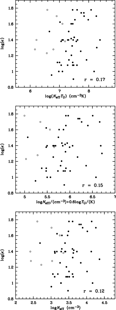
Figure 6: $\log\kappa$ versus $\log(N_{\rm eff}T_{\rm U}^{\nu})$ for PNe (filled circles) and H II regions (open circles), where $\nu=1$ (upper), 0.6 (middle), and 0(lower). The correlation coefficients are given in the lower right corner of each panel.

To reside in stationary states out of thermal equilibrium, the energetic electrons must be non-collisional. Collisionless plasma can be characterized by small ratio between the Debye length, $\lambda_{\rm D}\sim(T_{\rm U}/N_{\rm eff})^{0.5}$ and the mean free path, $L_{\rm m}\sim T_{\rm U}^{2}/N_{\rm eff}$, i.e., $\lambda_{\rm D}/L_{\rm m}$ ($\sim N_{\rm eff}^{0.5}/T_{\rm U}^{1.5}$) lower than one. Therefore, the $\kappa$ index should be related to the density and temperature of the system. Livadiotis (2015) found a negative correlation between $M$ [here, $M=1/(\kappa-0.5)$] and $\log(N_{\rm eff}T_{\rm U}^{\nu})$ for $\nu=1$, 0.6, and 0 (see their Figure 2). The sample examined by Livadiotis (2015) includes various space plasmas, but most of them are solar system plasmas. In Figure 6, we examine the correlation between $\log\kappa$ and $\log(N_{\rm eff}T_{\rm U}^{\nu})$ for our nebula sample. Although these best linear fits seem to show a trend that $\log\kappa$ increases with increasing $\log(N_{\rm eff}T_{\rm U}^{\nu})$, the point distributions in these diagrams are too scattering to definitely indicate a correlation. When comparing with Figure 2 of Livadiotis (2015), our data mostly concentrate in the right-down corner, namely the regions centred at $(\log N_{\rm eff}{[\rm m^{-3}]},M)=(9.5,0.05)$, $\log(N_{\rm eff}[\rm m^{-3}]T_{\rm U}^{0.6}[\rm K],M)=(11.8,0.05)$, and $\log(N_{\rm eff}[\rm m^{-3}]T_{\rm U}[\rm K],M)=(13.5,0.05)$. The $\kappa$ indices obtained in nebule are generally larger than those in solar system plasma. It should be noted that our plots are not contrary to those of Livadiotis (2015) as they examined a much wider parameter space. However, the non-existent correlation between the $\kappa$ index and the pair $(N_{\rm eff},T_{\rm U})$ in a smaller parameter space casts some doubts on whether $\kappa$ EEDs hold in PNe and H II regions.

ZLZ determined the $\kappa$ indices of four PNe through fitting their H I FB continuities. Three of them are included in our sample. However, the present method yields larger $\kappa$ indices for the three PNe than those obtained by ZLZ. Because the H I FB emission samples the electrons with lower energy than the [O III] CELs do, if the physical conditions of PNe are inhomogeneous we may obtained different results from the two methods. Therefore, it seems inappropriate to use a single $\kappa$ value to characterize the EED of a given PN. To further clarify this point, we need to investigate the behavior of other temperature diagnostic lines in $\kappa$ EEDs, such as the [N II] CEL ratio. The main difficulty to perform such a study is that the cross sections of collision are difficult to be tabulated, and thus are usually unavailable in the literature. Recently, Hahn & Savin (2015) presented a method to approximate $\kappa$ distributions as a sum of MB distributions, which provides an easy way to convert the existing rate coefficients with MB EEDs to those with $\kappa$ EEDs. The constraint of other CELs on the the $\kappa$ indices will be the subject of a forthcoming paper.

5 SUMMARY

Assuming that the discrepancy between $T_{\rm e}$(BJ) and $T_{\rm e}$([O III]) is completely attributed to non-thermal EEDs, we determine the $\kappa$ indices for a sample of PNe and H II regions. This is for the first time that the $\kappa$ indices for a large nebula sample are reported. These data provide a valuable resource for further research of the non-thermal electron distribution in space plasmas. Our results show that PNe have systematically lower $\kappa$ indices than H II regions, and the $\kappa$ indices in nebulae are significantly larger than those in solar system plasmas. Through an empirical fitting, we also present a convenient formula to deduce the $\kappa$ index from the $T_{\rm e}$(BJ)/$T_{\rm e}$([O III]) discrepancy.

Although the $\kappa$ EED provides a promising way to explain the long-standing RL/CEL discrepancy problem, its origin and physics validity should be thoroughly investigated. In order to explore the possible mechanisms that can cause the formation of the $\kappa$ distribution in photoionized gaseous nebulae, we examine the correlation between the obtained $\kappa$ indices and various other nebular properties. However, we cannot find sound evidence supporting that non-thermal electrons can be pumped in PNe and H II regions. For three extreme PNe, the currently obtained $\kappa$ indices are larger than those by ZLZ utilizing the H I FB continuum. In order to interpret this discrepancy within the framework of $\kappa$ EEDs, spatial variations of $\kappa$ and $T_{\rm U}$ are required. Given the scale of $\kappa$ distributions in the solar system, it is possible that such distributions may be present over small scales in nebular regions, and would be likely detected, should they exist, in nearby nebulae utilizing future high-resolution high-sensitivity facilities such as the James Webb Space Telescope (JWST).

Despite the difficulties to identify the orgin of non-thermal electrons, the present study cannot rule out the existence of the $\kappa$ distribution in PNe and H II regions. This scenario provides an intriguing possibility to solve some observational puzzles in nebulae. The $\kappa$ distribution can greatly affect thermal and ionization structures of nebulae and, if proven true, should be incorporated into photoionization models. One such attempt has been made by Dopita et al. (2013) who modified the photoionization code, MAPPINGS, to investigate the effect of $\kappa$ EEDs on abundance determination of H II regions. It would be a useful addition to applications such as Cloudy (Ferland et al., 2013), as a means of exploring the possible diagnostic symptoms of $\kappa$ EEDs. Apparently, it is extremely important to develop methods to detect EEDs from observations. We hope that the results reported in this paper can serve as a useful reference to further address this issue.

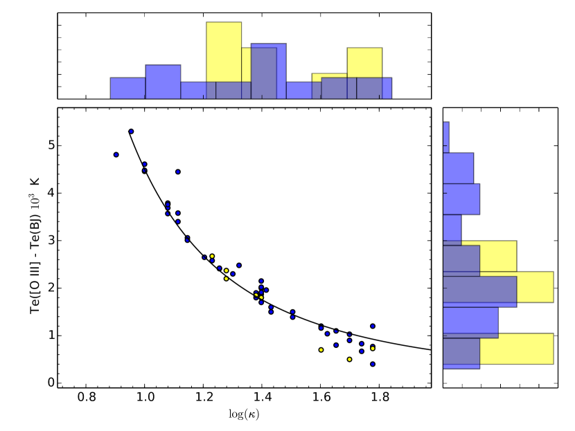
Figure 2: The electron temperature discrepancies, $T_{\rm e}$([O III])$-T_{\rm e}$(BJ), are plotted against the $\kappa$ values for PNe (blue) and H II regions (yellow). The histograms in the top and right panels show their distributions.

Table 1: The derived $\kappa$ values and other properties of PNe.

Object	Te(BJ)	Te([O III])	Ne	$\kappa$	TU	Neff	E.C.	ADF	Classa	Ref.
	(K)	(K)	(cm-3)		(K)	(cm-3)
BoBn 1	8840	13650	3370	8	10000	3000	1.6	2.63	S,iv	O10
Cn 1-5	10000	8770	3391	$\cdots$	$\cdots$	3391	3.9	1.02	B,ii	W07
Cn 2-1	10800	10250	10315	$\cdots$	$\cdots$	10315	$\cdots$	1.02	S,iii	W07
Cn 3-1	5090	7670	6830	17	5500	6494	$\cdots$	$\cdots$	E,ii	W05
DdDm 1	8730	12300	4500	12	9500	4180	1.7	11.80	E,iv	W05
H 1-35	12000	9060	22585	$\cdots$	$\cdots$	22585	2.3	1.04	S,iv	W07
H 1-41	4500	9800	1125	9	5300	1016	3.9	5.11	S,iii	W07
H 1-42	10000	9690	7508	$>$60	$\cdots$	7508	4.2	1.04	B,ii	W07
H 1-50	12000	10950	9355	$\cdots$	$\cdots$	9355	5.0	1.05	E,ii	W07
H 1-54	12500	9540	13032	$\cdots$	$\cdots$	13032	2.0	1.05	B,iv	W07
He 2-118	14500	12630	15155	$\cdots$	$\cdots$	15155	$\cdots$	1.03	S,iii	W07
Hu 1-1	8350	12110	1360	12	9100	1263	4.7	2.97	E,ii	W05
Hu 1-2	18900	19500	4467	$\cdots$	$\cdots$	4467	3.4	1.60	B,ii	L04
Hu 2-1	8960	9860	7870	50	9000	7742	1.9	4.00	B,ii	W05
IC 351	11050	13070	2630	25	11600	2543	4.9	3.14	E,ii	W05
IC 1747	9650	10850	2980	40	9800	2919	5.1	3.20	E,ii	W05
IC 2003	8960	12650	3130	12	9800	2908	4.4	7.31	E,ii	W05
IC 3568	9490	11400	1995	25	10000	1929	4.8	2.20	R,ii	L04
IC 4191	9200	10000	10695	45	9200	10501	5.0	2.40	B,ii	T03
IC 4406	9350	10000	1560	$>$60	$\cdots$	1560	4.7	1.90	B,ii	T03
IC 4699	12000	11720	2119	$\cdots$	$\cdots$	2119	5.5	1.09	E, $\cdots$	W07
IC 4846	7700	10710	10960	14	8200	10299	4.3	2.91	B,iii	W05
IC 5217	11350	11270	4510	$\cdots$	$\cdots$	4510	$\cdots$	2.26	E,iii	W05
M 1-20	12000	9860	10151	$\cdots$	$\cdots$	10151	4.3	1.02	E,ii	W07
M 1-29	10000	10830	6297	55	11000	6204	6.5	2.95	E,ii	W07
M 1-61	9500	8900	20817	$\cdots$	$\cdots$	20817	4.0	1.03	R,ii	W07
M 1-73	5490	7450	4490	26	5800	4347	1.3	3.61	B, $\cdots$	W05
M 1-74	7850	10150	24030	20	8200	23032	4.4	2.14	R,ii	W05
M 2-4	7900	8570	7041	55	8000	6937	3.5	1.88	S,ii	W07
M 2-6	11700	10100	7523	$\cdots$	$\cdots$	7523	3.1	1.04	E,ii	W07
M 2-27	14000	11980	11217	$\cdots$	$\cdots$	11217	4.2	1.04	E,iii	W07
M 2-31	14000	9840	6141	$\cdots$	$\cdots$	6141	$\cdots$	$\cdots$	R, $\cdots$	W07
M 2-33	7000	8040	1501	42	7100	1471	2.7	2.150	E,iv	W07
M 2-36	5900	8380	4230	21	6700	4063	3.6	6.90	B,ii	L01
M 2-42	14000	8470	3430	$\cdots$	$\cdots$	3429	3.6	1.04	E,iii	W07
M 3-7	6900	7670	4093	60	7000	4037	2.0	4.40	R,iv	W07
M 3-21	10400	9790	13652	$\cdots$	$\cdots$	13652	$\cdots$	1.05	E,ii	W07
M 3-29	10700	9190	813	$\cdots$	$\cdots$	813	2.5	1.04	E,ii	W07
M 3-32	4400	8860	2085	10	5000	1905	3.2	17.75	E,iv	W07
M 3-33	5900	10380	2068	10	6700	1889	4.9	6.56	E,iii	W07
M 3-34	8440	12230	3500	12	9400	3251	5.7	4.23	S, $\cdots$	W05
Me 2-2	10590	10970	11930	$>$60	$\cdots$	11930	$\cdots$	2.10	B,ii	W05
NGC 40	7020	10600	1202	13	7600	1123	0.2	17.80	E,ii	L04
NGC 1501	9400	11100	1312	25	9800	1268	4.9	32.00	E,i	E04
NGC 2022	13200	15000	1505	25	14000	1455	3.3	16.00	B,ii	T03
NGC 2440	14000	16150	$\cdots$	25	15000	$\cdots$	8.3	5.40	E,ii	T03
NGC 2867	8950	11600	2850	16	9500	2700	6.2	1.63	B, ii	G09
NGC 3132	10780	9530	600	$\cdots$	$\cdots$	600	3.6	3.50	B,ii	T03
NGC 3242	10200	11700	2070	27	16000	2006	5.7	2.20	B,ii	T03
NGC 3918	12300	12600	5667	$>$60	$\cdots$	5667	6.6	2.30	B,ii	T03
NGC 5307	10700	11800	3133	45	11000	3076	5.2	1.95	B,i	R03
NGC 5315	8600	9000	14091	60	8700	13900	3.6	2.00	B,i	T03
NGC 5882	7800	9400	4113	27	8000	3987	4.7	2.10	B,ii	T03
NGC 6153	6080	9140	3400	14	6600	3195	4.0	9.20	E,i	L00
NGC 6210	9300	9680	4365	$>$60	$\cdots$	4365	3.5	3.10	B,iii	L04
NGC 6302	16400	18400	14000	25	18000	13538	8.5	3.60	B,i	T03
NGC 6439	9900	10360	5169	$>$60	$\cdots$	5169	5.7	6.16	E,iii	W07
NGC 6543	8340	8000	4770	$\cdots$	$\cdots$	4770	3.1	4.20	B,i	W04
NGC 6565	8500	10300	1329	24	8900	1283	5.7	1.69	E,ii	W07
NGC 6567	14000	10580	8118	$\cdots$	$\cdots$	8118	4.2	1.04	E,iii	W07
NGC 6572	11000	10600	15136	$\cdots$	$\cdots$	15136	$\cdots$	1.60	B,ii	L04
NGC 6620	8200	9590	2535	32	8400	2470	5.8	3.19	R,ii	W07
NGC 6720	9100	10600	501	32	9300	488	4.8	2.40	E,ii	L04
NGC 6741	15300	12600	5129	$\cdots$	$\cdots$	5129	6.3	1.90	E,ii	L04
NGC 6790	15000	12800	39811	$\cdots$	$\cdots$	39811	$\cdots$	1.70	B,ii	L04
NGC 6803	7320	9740	7190	18	7800	6857	4.9	2.71	E,ii	W05
NGC 6807	9900	10930	18530	50	10000	18229	4.3	2.00	R,iv	W05
NGC 6818	12140	13300	2063	40	12500	2020	7.7	2.90	E,ii	T03
NGC 6826	9650	9370	1995	$\cdots$	$\cdots$	1995	3.4	1.90	E,ii	L04
NGC 6833	13670	12810	19030	$\cdots$	$\cdots$	19030	$\cdots$	2.47	B,iv	W05
NGC 6879	8500	10400	4380	24	8900	4229	4.4	2.46	R,ii	W05
NGC 6884	11600	11000	7413	$\cdots$	$\cdots$	7412	5.3	2.30	E,ii	L04
NGC 6891	5930	9330	1660	13	6500	1551	3.3	1.52	E,ii	W05
NGC 7009	6490	10940	4290	13	7100	4010	5.2	5.00	B,ii	F11
NGC 7026	7440	9310	5510	25	7800	5328	4.1	3.36	B,ii	W05
NGC 7027	12800	12600	52289	$>$60	$\cdots$	51589	7/0	1.29	B,ii	Z05
NGC 7662	12200	13400	3236	60	12600	3192	6.8	2.00	E,ii	L04
PB 8	5100	6900	2550	25	5400	2465	1.6	1.05	E,ii	G09
Sp 4-1	8830	11240	1880	18	9300	1792	2.3	2.94	B, $\cdots$	W05
Vy 1-2	6630	10400	2850	12	7200	2647	6.0	6.17	E,iv	W05
Vy 2-1	8700	7860	3815	$\cdots$	$\cdots$	3815	2.8	1.03	E,ii	W07
Vy 2-2	9300	13910	16130	10	10400	14740	2.9	11.80	S,iv	W05

References. — (E04) Ercolano et al. 2004; (F11) Fang & Liu 2011; (G09) García-Rojas et al. 2009; (L00) Liu et al. 2000; (L01) Liu et al. 2001; (L04) Liu et al. 2004; (O10) Otsuka et al. 2010; (R03) Ruiz et al. 2003; (T03) Tsamis et al. 2003a; (W07) Wang & Liu 2007; (W04) Wesson & Liu 2004; (W05) Wesson et al. 2005; (Z05) Zhang et al. 2005.

Table 2: The derived $\kappa$ values and other properties of H II regions.

Object	Te(BJ)	Te([O III])	Ne	$\kappa$	TU	Neff	ADF	Ref.
	(K)	(K)	(cm-3)		(K)	(cm-3)
30 Dor	9220	9950	416	60	9400	410	1.62	P03
H 1013	5000	7700	280	19	5400	270	2.29	B07,E09
M 8	7100	7800	1800	40	7200	1760	2.0	G05
M 16	5450	7650	1120	19	5800	1070	2.8	G07
M 17	7700	8200	1050	50	7800	1030	2.1	T03
M 20	6000	7980	270	25	6300	260	2.1	G07
M 42	7900	8300	6350	$>60$	8000	6260	1.02	E04
NGC 3576	6650	8500	2300	24	7000	2220	1.8	G07
NGC 5447	6610	9280	560	17	7000	530	1.55	E09
S 311	9500	9000	310	…	…	310	1.03	G05

References. — (B07) Bresolin 2007; (E04) Esteban et al. 2004; (E09) Esteban et al. 2009; (G05) García-Rojas et al. 2005; (G07) García-Rojas & Esteban 2007; (P03) Peimbert 2003; (T03) Tsamis et al. 2003b.

References

- Bresolin (2007) Bresolin, F. 2007, ApJ, 656, 186
- Cranmer (2014) Cranmer, S. R. 2014, ApJ, 791, L31
- Dopita & Meatheringham (1990) Dopita, M. A., & Meatheringham, S. J. 1990, ApJ, 357, 140
- Dopita et al. (2013) Dopita, M. A., Sutherland, R. S., Nicholls, D. C., Kewley, L. J., & Vogt, F. P. A. 2013, ApJS, 208, 10
- Ercolano et al. (2004) Ercolano, B., Wesson, R., Zhang, Y., et al. 2004, MNRAS, 354, 558
- Esteban et al. (2004) Esteban, C., Peimbert, M., García-Rojas, J., et al. 2004, MNRAS, 355, 229
- Esteban et al. (2009) Esteban, C., Bresolin, F., Peimbert, M., et al. 2009, ApJ, 700, 654
- Fang & Liu (2011) Fang, X., & Liu, X.-W. 2011, MNRAS, 415, 181
- Ferland et al. (2013) Ferland, G. J., Porter, R. L., van Hoof, P. A. M., et al. 2013, Rev. Mexicana Astron. Astrofis., 49, 137
- Feldman et al. (1975) Feldman, W. C., Asbridge, J. R., Bame, S. J., Montgomery, M. D., & Gary, S. P. 1975, J. Geophys. Res., 80, 4181
- García-Rojas & Esteban (2007) García-Rojas, J., & Esteban, C. 2007, ApJ, 670, 457
- García-Rojas et al. (2005) García-Rojas, J., Esteban, C., Peimbert, A., et al. 2005, MNRAS, 362, 301
- García-Rojas et al. (2013) García-Rojas, J., Peña, M., Morisset, C., et al. 2013, A&A, 558, A122
- García-Rojas et al. (2009) García-Rojas, J., Peña, M., & Peimbert, A. 2009, A&A, 496, 139
- Hahn & Savin (2015) Hahn, M., & Savin, D. W. 2015, ApJ, 809, 178
- Humphrey & Binette (2014) Humphrey, A., & Binette, L. 2014, MNRAS, 442, 753
- Leubner (2002) Leubner, M. P. 2002, Ap&SS, 282, 573
- Liu (2006) Liu, X.-W. 2006, in IAU Symp. 234 Planetary Nebulae, eds. M. J. Barlow, & R. H. Méndez (Cambridge: Cambridge Univ. Press), 219
- Liu et al. (2006) Liu, X.-W., Barlow, M. J., Zhang, Y., Bastin, R. J., & Storey, P. J. 2006, MNRAS, 368, 1959
- Liu et al. (2001) Liu, X.-W., Luo, S.-G., Barlow, M. J., Danziger, I. J., & Storey, P. J. 2001, MNRAS, 327, 141
- Liu et al. (2004) Liu, Y., Liu, X.-W., Luo, S.-G., & Barlow, M. J. 2004, MNRAS, 353, 1231
- Liu et al. (2000) Liu, X.-W., Storey, P. J., Barlow, M. J., et al. 2000, MNRAS, 312, 585
- Livadiotis (2015) Livadiotis, G. 2015, J. Geophys. Res., 120, 1607
- Livadiotis & McComas (2009) Livadiotis, G., & McComas, D. J. 2009, J. Geophys. Res., 114, 1110
- Nicholls et al. (2012) Nicholls, D. C., Dopita, M. A., & Sutherland, R. S. 2012, ApJ, 752, 148
- Nicholls et al. (2013) Nicholls, D. C., Dopita, M. A., Sutherland, R. S., Kewley, L. J., & Palay, E. 2013, ApJS, 207, 21
- Otsuka et al. (2010) Otsuka, M., Tajitsu, A., Hyung, S., & Izumiura, H. 2010, ApJ, 723, 658
- Peimbert (1978) Peimbert, M. 1978, in Planetary Nebulae, Observation and Theory, ed. Y., Terzian (Dordrecht: Reidel), IAU Symp., 76, 215
- Peimbert (2003) Peimbert, A. 2003, ApJ, 584, 735
- Quireza et al. (2007) Quireza, C., Rocha-Pinto, H. J., & Maciel, W. J. 2007, A&A, 475, 217
- Ruiz et al. (2003) Ruiz, M. T., Peimbert, A., Peimbert, M., & Esteban, C. 2003, ApJ, 595, 247
- Seely et al. (1987) Seely, J. F., Feldman, U., & Doschek, G. A. 1987, ApJ, 319, 541
- Storey & Sochi (2013) Storey, P. J., & Sochi, T. 2013, MNRAS, 430, 598
- Storey & Sochi (2014) Storey, P. J., & Sochi, T. 2014, MNRAS, 440, 2581
- Storey & Sochi (2015a) Storey, P. J., & Sochi, T. 2015a, MNRAS, 446, 1864
- Storey & Sochi (2015b) Storey, P. J., & Sochi, T. 2015b, MNRAS, 449, 2974
- Tsamis et al. (2003a) Tsamis, Y. G., Barlow, M. J., Liu, X.-W., Danziger, I. J., & Storey, P. J. 2003a, MNRAS, 345, 186
- Tsamis et al. (2003b) Tsamis, Y. G., Barlow, M. J., Liu, X.-W., Danziger, I. J., & Storey, P. J. 2003b, MNRAS, 338, 687
- Vasyliunas (1968) Vasyliunas, V. M. 1968, J. Geophys. Res., 73, 2839
- Wang & Liu (2007) Wang, W., & Liu, X.-W. 2007, MNRAS, 381, 669
- Wesson & Liu (2004) Wesson, R., & Liu, X.-W. 2004, MNRAS, 351, 1026
- Wesson et al. (2005) Wesson, R., Liu, X.-W., & Barlow, M. J. 2005, MNRAS, 362, 424
- Zhang et al. (2005) Zhang, Y., Liu, X.-W., Luo, S.-G., Péquignot, D., & Barlow, M. J. 2005, A&A, 442, 249
- Zhang et al. (2004) Zhang, Y., Liu, X.-W., Wesson, R., et al. 2004, MNRAS, 351, 935
- Zhang et al. (2014) Zhang, Y., Liu, X.-W., & Zhang, B. 2014, ApJ, 780, 93