Atom-Field Entanglement in Cavity QED: Nonlinearity and Saturation

Abstract

We investigate the degree of entanglement between an atom and a driven cavity mode in the presence of dissipation. Previous work has shown that in the limit of weak driving fields, the steady state entanglement is proportional to the square of the driving intensity. This quadratic dependence is due to the generation of entanglement by the creation of pairs of photons/excitations. In this work we investigate the entanglement between an atom and a cavity in the presence of multiple photons. Nonlinearity of the atomic response is needed to generate entanglement, but as that nonlinearity saturates the entanglement vanishes. We posit that this is due to spontaneous emission, which puts the atom in the ground state and the atom-field state into a direct product state. An intermediate value of the driving field, near the field that saturates the atomic response, optimizes the atom-field entanglement. In a parameter regime for which multiphoton resonances occur, we find that entanglement recurs at those resonances. In this regime, we find that the entanglement decreases with increaing photon number. We also investigate, in the bimodal regime, the entanglement as a function of atom and/or cavity detuning. Here we find that there is evidence of a phase transition in the entanglement, which occurs at $2\epsilon/g\geq 1$.

I Introduction

Over the last two decades studies into the foundations of quantum mechanics have shown that entanglement is an inherently quantum mechanical property that, among other things, is useful for description of prime product factorization, search protocols, and quantum teleportation Nielsen and Chuang (2000); Jaeger (2007). The measure of entanglement is well defined in the case of two interacting qubits. Consider a two qubit state

$$|\psi\rangle=C_{00}|00\rangle+C_{01}|01\rangle+C_{10}|10\rangle+C_{11}|11\rangle$$ (1)

If a system is in the product state

$$|\psi\rangle=(A_{0}|0\rangle+A_{1}|1\rangle)(B_{0}|0\rangle+B_{1}|1\rangle)$$ (2)

then the probability amplitudes will satisfy

$$\mathcal{E}\equiv C_{00}C_{11}-C_{01}C_{10}=0$$ (3)

If this relation is not satisfied then the state is entangled. The concurrence $\mathcal{C}=\sqrt{2\mathcal{E}}$ is a measure of entanglement for two qubits Hill and Wootters (1997); Wootters (1998). The log negativity $\mathcal{E}_{N}$ is another measure of entanglement that presents an upper bound to the entanglement of distillation and is conveniently additive Vidal and Werner (2002). In the simple case of two qubits $\mathcal{E}_{N}=\log_{2}(||\rho^{T_{F}}||)=\log_{2}(1+\sqrt{2}\mathcal{E)}$.

Three qubits can be entangled in several ways. The qubits can be in a Greenburger-Horne-Zeilinger Greenberger (1990) state, a W state Dür et al. (2000), or the entanglement can be solely between various bipartite splits of the system (i.e. particle 1 entangled with 2 and 3 etc. ) Coffman et al. (2000). A system of two coupled qubits that interact with an environment via pumping and/or dissipation is similar to a three-qubit system. In this case, the system is essentially tri-partite: qubit 1, qubit 2, and the environment. If we choose to trace or average over the environmental degrees of freedom, the two qubits will be described by a mixed state instead of a pure state.

There are many ways to measure entanglement Horodecki et al. (2009), many of which require optimization of a convex function. In this paper we adopt a pragmatic approach, introduced by Nha and Carmichael Nha and Carmichael (2004), that utilizes quantum trajectory theory. Open quantum systems can be described by a reduced density matrix that is obtained by tracing over environmental degrees of freedom. Recall that in quantum trajectory theory, the density matrix takes the form

$$\dot{\rho}=\mathcal{L}\rho=(\mathcal{L-S})\rho+\mathcal{S}\rho$$ (4)

where $\mathcal{L}$ is the Liouvillian operator defined by the master equation, and $\mathcal{S}$ is any combination of system operators. For a given choice of $\mathcal{S}$, the $\mathcal{L-S}$ part of the evolution can be described by an effective Schroedinger equation, with a non-Hermitian Hamiltonian evolving the conditioned state $|\psi_{c}\rangle$. This is referred to as a quantum trajectory Carmichael (1993); Mølmer and Castin (1996); Tian and Carmichael (1992). This evolution is punctuated by the application of the $\mathcal{S}$ operator, which we refer to as a jump, at times randomly chosen from a distribution that is determined by the current state of the system. At every time step the trajectory must be normalized, as a jump or non-Hermitian evolution results in nonunitary evolution. To fully recover the statistical information about the system, one then averages over a set of trajectories. Obviously, a different choice for $\mathcal{S}$ leads to a different unraveling and a different set of trajectories. One common choice for $\mathcal{S}$ is that of direct detection, where, for example, the spontaneous emission of an atom is monitored via a $4\pi$ detector with perfect efficiency. This yields quantum trajectories conditioned on this measurement record. Another common choice is that of homodyne detection, where the number of jumps is very high over the characteristic dissipatiive/driving rates of the system and one coarse grains the resulting equation, resulting in a nonlinear Schroedinger equation for evolution.

Good reviews of this topic and its relationship to measurement theory can be found in the works of Wiseman Wiseman (1996) and Jacobs and Steck Jacobs and Steck (2006). Nha and Carmichael proposed applying pure state entanglement measures to the quantum trajectories, yielding a functional definition of entanglement for open systems. They explicitly demonstrated that the ”amount” of entanglement may be different for different choices of $\mathcal{S}$ by examining the results given by homodyne and direct detection applied to their optical system. For weak fields the unraveling is irrelevant, as the system is well approximated by a pure state for many lifetimes, as the jump rate $P(t)dt=\gamma\langle\sigma_{z}(t)+1/2\rangle dt$ and $\sigma_{z}(t)\approx-1$ for weak fields, so jump events are relatively rare. It has been shown that while entanglement is different for different unravelings, for a given unraveling all measures of entanglement show similar behavior as system parameters are changed Guevara and Viviescas (2014).

In this paper we use this method of examining entanglement in open quantum systems and choose jump operators corresponding to direct detection. We take the point of view that a quantum trajectory based on direct detection monitoring could aid in understanding the amount of useful entanglement in a quantum information processing protocol that utilizes direct detection for state preparation and processing.

In Section II we describe the system to be studied. In Section III, results for weak driving fields are presented and the validity of the weak driving-field approximation is examined. The behavior of the log negativity for a system driven on resonance with a field of arbitrary strength is treated in Section IV. Results for the behavior of the log negativity for a system driven off resonance by fields of a variety of strengths are presented in Sections V and VI.

II System Description

We use a python toolkit for modeling the dynamics of open quantum systems Johansson et al. (2012, 2013). The system we investigate is a single two-level atom located at an anti-node of a field mode in an optical cavity, as shown in Fig. 1. The cavity is driven by a photon flux $\epsilon$, one end mirror is ”leaky” with a field dissipation rate of $\kappa$, and the atom spontaneously emits out the side of the cavity at the cavity-modified rate $\gamma$. The coupling between the field mode and the atom is given by $g$.

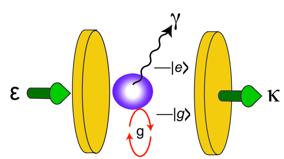
Figure 1: Single atom in a driven optical cavity with dipole coupling $g$, cavity field loss rate $\kappa$, and atomic spontaneous emission rate $\gamma$.

The quantum trajectory wave function and Hamiltonian that characterize the system are:

$$|\psi_{c}(t)\rangle = \left.\sum_{n}^{\infty}(C_{g,n}(t)e^{-iE_{g,n}t}|g,n\rangle+C_{e,n}(t)e^{-iE_{e,n}t}|e,n\rangle)\right.$$ (5)

$$H = \frac{\hbar}{2}\Delta\sigma_{z}+\hbar\theta a^{\dagger}a+\hbar g\hskip 2.70004pt(a^{\dagger}\sigma_{-}+a\sigma_{+})-i\hbar\kappa a^{\dagger}a-i\hbar\frac{\gamma}{2}\sigma_{+}\sigma_{-}+i\hbar\epsilon(a^{\dagger}-a)$$ (6)

with collapse operators

$$\mathcal{A} = \sqrt{\kappa}a$$ (7)

$$\mathcal{S} = \sqrt{\frac{\gamma}{2}}\sigma_{-}.$$ (8)

associated with detection of photons exiting the output mirror and out the side of the cavity, respectively. The indices $e$ and $g$ indicate the atom in the excited or ground state, while $n$ is the number of photons in the mode. The creation and annihilation operators for the field are $a^{\dagger}$ and $a$, and the Pauli raising and lowering operators for the atom are $\sigma_{+}$ and $\sigma_{-}$. The detunings are given by $\Delta=2(\omega_{atom}-\omega_{cav})/\gamma$ and $\theta=(\omega_{drive}-\omega_{cav})/\kappa$.

III Weak Driving Field

In the weak driving-field limit, the system reaches a steady-state wave function of the form

$$|\psi_{WF}\rangle=|0g\rangle+A_{1,g}|1g\rangle+A_{0,e}|0e\rangle+A_{2,g}|2g\rangle+A_{1,e}|1e\rangle$$ (9)

where the $A_{i,j}$ are known Carmichael et al. (1991); Brecha et al. (1999).

To lowest order in the weak driving-field approximation, $A_{1,g}$ and $A_{0,g}$ are proportional to the driving field strength $\epsilon$. A quantity that is key to understanding entanglement in the weak field limit is

$$\frac{A_{1,e}}{A_{1,g}A_{0,e}}=q=\frac{(1+2C_{1})}{(1+2C_{1}-2C^{{}^{\prime}}_{1})}$$ (10)

with $C_{1}=g^{2}/\kappa\gamma$ and $C_{1}^{\prime}=2C_{1}\kappa/(2\kappa+\gamma)$. As noted above, the one-excitation amplitudes $A_{1,g}$ and $A_{0,e}$ are proportional to the driving field $\epsilon$ and the two-excitation amplitudes, $A_{2,g}$ and $A_{1,e}$, are proportional to the square of the driving field, $\epsilon^{2}$. Carmichael et al. (1991); Brecha et al. (1999).

The key quantity $q$ is related to the cross correlation

$$g^{(2)}_{TF}(0)=\frac{\langle a^{\dagger}a\sigma_{+}\sigma_{-}\rangle}{\langle a^{\dagger}a\rangle\langle\sigma_{+}\sigma_{-}\rangle}=q,$$ (11)

which is the probability of simultaneous detection of transmitted and fluorescence photons scaled by the product of the probability of two independent detections in transmission and fluorescence.

In the weak-field limit, $\epsilon/\kappa\ll 1$, the concurrence for this system is found to be

$$\mathcal{C}=-\left(\frac{\epsilon}{\kappa}\right)^{4}\log_{2}\left[\left(\frac{\epsilon}{\kappa}\right)^{4}\right]\xi^{2},$$ (12)

where

$$\xi=\frac{2g}{\gamma(1+2C_{1})^{2}}(q-1).$$ (13)

These relations hold provided $(\epsilon/\kappa)^{2}\ll|\xi|<1$. The log negativity is found simply from the concurrence.

We now investigate the range of validity of the weak-field approximations given above. Figure 2 shows the fidelity $\mathcal{F}$ defined as

$$\mathcal{F}=\operatorname{Tr}(1-\rho_{c}^{2})$$ (14)

We have performed an average over many trajectories to obtain an ensemble average. We see that a pure state approximation is valid for driving fields well below the strength of the saturation field. We also plot the norm of the distance between the state we calculate using trajectories for an arbitrary field strength and the pure state obtained in the weak field limit. This norm $\mathcal{D}$ has the form

$$\mathcal{D}=|\langle\psi_{WF}|\psi_{c}\rangle|^{2}$$ (15)

Again we find good agreement for field strengths up to half the saturation field. That this agreement is sensible can be understood as follows. The large component of the state corresponds to the vacuum state of the field and the ground state of the atom. Hence, at field strengths below half the saturation field, the mean photon number is very small (close to zero), and the atomic inversion is very close to $-1$, i.e. the atom in the ground state. Hence, the purity of the state is not unexpected for low field strengths, though the similarity between the actual state and the weak field state approximation is, perhaps, a bit surprising. However, we posit that $|\psi_{c}\rangle=|0\rangle+d|\text{1-excitation}\rangle$ and $|\psi_{WF}\rangle=|0\rangle+d^{\prime}|\text{1-excitation}\rangle$ giving a distance that is approximately $|d-d^{\prime}|$, which is proportional to $\epsilon^{2}$ and so is small compared to $1$ for weak driving fields. Also, as the driving field strength becomes larger, the state of the system is no longer in a quasi-steady state for many lifetimes as it would be in the weak driving field approximation and the rate of spontaneous emission jumps is on the order of the lifetime. The spontaneous emission rate is greatest at saturation and each spontaneous emission event destroys entanglement.

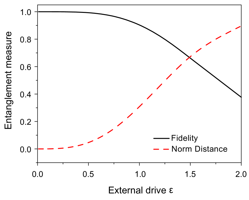
Figure 2: Comparison of the wavefunction to the one obtained analytically in the week field limit via two measures, the fidelity and norm of the distance, both defined in the text.

IV Log Negativity on Resonance

We now consider entanglement in the presence of driving fields of arbitrary strength that are resonant with both the atom and the cavity. In Fig. 3, we plot the population inversion of the atom and intracavity photon number as a function of resonant driving field, with coupling and dissipation rates of similar magnitude, and with the driving field scaled so that when $\epsilon=1$, the intensity in the cavity is equal to the saturation intensity of the atom. We see typical behavior, the photon number rising as the driving field is increased and becoming linear for high fields after the atom saturates Bonifacio and Lugiato (1978). Low and high fields in this case being $\epsilon\ll 1$ and $\epsilon\gg 1$ respectively. The atomic inversion increases with increasing driving field and pins at the value of zero for high fields.

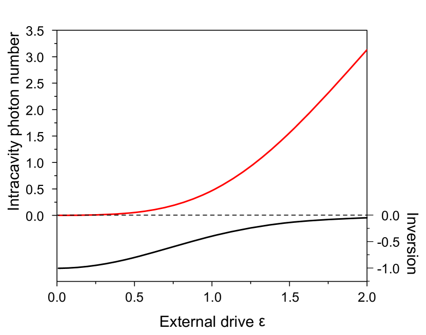
Figure 3: Average intracavity photon number and atomic population inversion as a function of driving field for $\kappa=\gamma=g=1.0$.

We use as our measure of entanglement the logarithmic negativity defined as

$$\mathcal{E}_{N}=\log_{2}(\|\rho^{T_{F}}\|).$$ (16)

Here $\|\rho^{T_{F}}\|$ is the trace norm of the partial transpose of the density matrix with respect to the field, which is formed in the following manner. The wavefunction from our trajectory theory is used to calculate a density matrix for the atom-field system. This is then used in constructing $\rho^{T_{F}}$. We truncate the basis for the Fock states of the field mode at a number well above the average photon number as predicted by semiclassical theories, and then adjust that upper truncation level to assure that our results are insensitive to that truncation. We obtain similar results using the negativity $\mathcal{N}=(1/2)(||\rho^{T_{F}}||-1)$ and concurrence $\mathcal{C}$; we use the log negativity for ease of calculation.

Figure 4(a) shows the temporal development of the log negativity as a function of time for a variety of driving field strengths. Here we see a well defined steady-state entanglement value, with a preceding maximal value. There are also oscillations that are roughly at the Rabi frequency for larger driving fields, and which are written into the dynamics via the eigenvalues of the time evolution operator. In Figure 4(b), we plot the log negativity as a function of driving strength for several times. We see that at long enough times, there is indeed an optimal driving field near $\epsilon=1$.

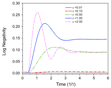
(a)

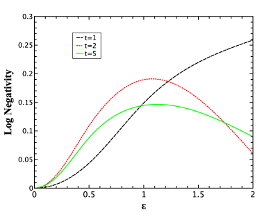
(b)

Figure 4: (a) Log negativity as a function of time for various driving field strengths. (b) Log negativity as a function of driving field strength for $\gamma t=1.0$, $2.0$, and $5.0$.

Figure 5 shows the log negativity as a function of the driving field strength. We plot both the steady state value, reached several atomic/cavity lifetimes after the system is started in the ground state, as well as the maximum value obtained over that same time period. We find that the optimum value for the driving field strength is equal to the field that would saturate the atom, $\epsilon\approx 1.0$. Beyond that field strength the entanglement decreases, ultimately to zero.

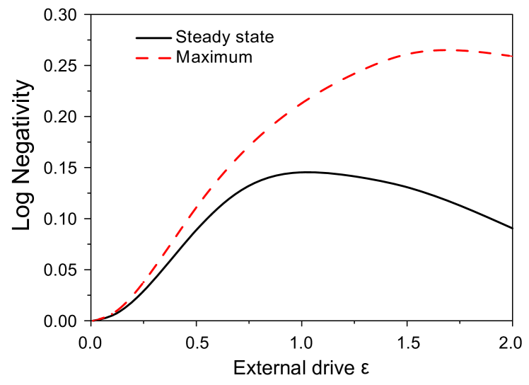
Figure 5: Maximum and steady-state value of the log negativity as a function of field strength.

As two oscillators coupled together with a linear coupling will not become entangled, we know that the nonlinearity of the atom is crucial to the formation of atom-field entanglement. However, when that nonlinearity saturates, the entanglement decreases. If one replaces the atom with a harmonic oscillator, it is driven to a coherent state and $q=1$. Essentially the atom is in a mixed state with equal probabilities of being in the excited and ground states, and the atom-field state factorizes. The physical mechanism responsible for the loss of entanglement is spontaneous emission, which is maximized for a saturated atom.

V Log Negativity Off Resonance

The entanglement off resonance and for relatively high driving fields is examined in this section. In Fig. 6 we see that the general behavior in which the log negativity vanishes as the atom saturates holds over different field-cavity detunings $\theta$. However, when $\theta\neq 0$ there is an asymmetry, and the log negativity persists at slightly higher driving fields.

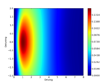
(a)

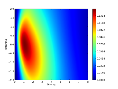
(b)

Figure 6: The log-negativity with (a) $\theta=0$ and (b) $\theta=0.5$ . Parameters used are $\kappa,\gamma$ and $g=1$. 100 states of the cavity are kept.

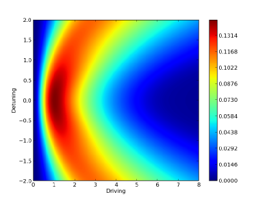
(a)

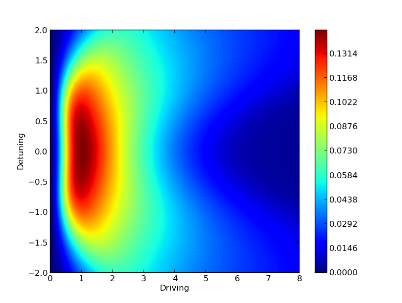
(b)

Figure 7: The log-negativity with (a) $\theta=-\Delta$ and (b) $\theta=\Delta$. Parameters used are $\kappa,\gamma$ and $g=1$.

Figure 7 shows that when $\theta=\pm\Delta$ this persistence is either enhanced or suppressed. Explanation for this behavior can be found in the examination of the effect $\Delta$ and $\theta$ have on the vacuum Rabi frequency. Following Brecha, Rice, and Xiao Brecha et al. (1999) we note that including these detunings effectively makes $\kappa$ and $\gamma$ complex,

$$\kappa\to\kappa(1+i\theta)=\tilde{\kappa}$$ (17)

$$\gamma\to\gamma(1+i\Delta)=\tilde{\gamma}.$$ (18)

The vacuum Rabi frequency becomes

$$\tilde{\Omega}=\sqrt{\left(\frac{1}{4}\right)\left(\tilde{\kappa}-\frac{\tilde{\gamma}}{2}\right)^{2}-g^{2}}$$ (19)

Note that the relative signs of $\kappa$ and $\gamma$ matter a great deal. If $\theta=-\Delta$ the terms enhance one another, and hence we observe the behavior in Fig. 7(a) while, if the $\theta=\Delta$, we see behavior similar to driving on resonance, producing the results in Fig. 7(b). The behavior in Fig. 7(a) is due to the persistence of vacuum Rabi oscillations when the detunings ”cancel” in this manner. One effectively tunes to a vacuum Rabi sideband, and sees two-level behavior as in Tian et. al. Tian and Carmichael (1992).

VI Strong Coupling and Driving Off Resonance

In this section the behavior of the system for extremely high coupling between the cavity and atom is examined. Though the results presented above seem to imply that entanglement vanishes for fields much larger than the field that saturates the atom, we instead find that, when coupling is of sufficiently high magnitude, there is a regime where the entanglement reappears. This behavior in the average photon number has been noted before, and is due to the $g\sqrt{n}$ Rabi splitting via strong coupling and/or high driving fields. In general, these conditions give rise to multi-photon processes Shamailov et al. (2010). As various multi-photon resonances are obtained, there is a regime in which the system effectively behaves like a two-level system, resulting in entanglement as in the resonant weak driving-field case. The results of our calculations are shown in Fig. 8.

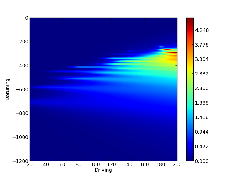
(a)

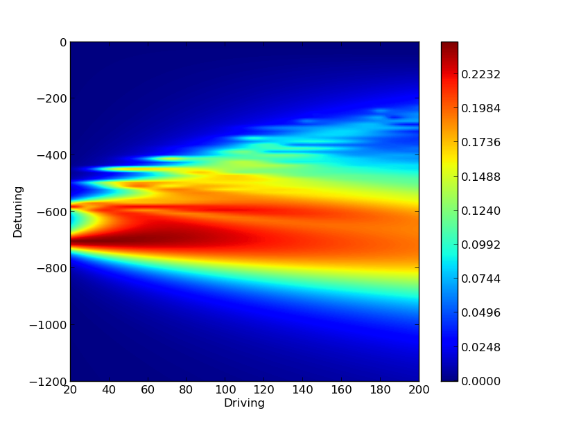
(b)

Figure 8: Intracavity photon number (a) and log negativity (b) for high driving fields with $\theta=\Delta$. Parameters used are $\kappa=1$, $\gamma=2$, and $g=1000$. 15 states of the cavity kept.

Notice that for larger photon number, the accompanying entanglement is smaller. This is due to the increase of the excited state population of the effective two level system with increasing intracavity photon number. Again, there is less entanglement if the atom saturates.

Another regime of interest is near the phase transition that occurs where $2\epsilon/g=1$ Alsing and Carmichael (1991); Alsing et al. (1992); Carmichael (2015). The entanglement in this regime has been studied by Gea-Banacloche et. al. Gea-Banacloche et al. (2005) outside the secular approximation used by Alsing et. al. Alsing et al. (1992); Alsing and Carmichael (1991), where one ignores the difference between oscillations at $\sqrt{(\langle n\rangle\pm\langle n\rangle^{1/2})}g$. We do not make the secular approximation, and we find that the atom and field are entangled in the regime where $2\epsilon/g>1$, with a sharp demarcation between this regime and the regime at fields below the phase transition. As for weak fields, when one drives the system to saturation, spontaneous emission kills the entanglement. This behavior is depicted in Fig. 9. One anticipates the presence of entanglement noting that Gea-Banacloche et. al. Gea-Banacloche et al. (2005) found that while no steady state exists, for individual trajectories one finds

$$|\psi\rangle_{ss}=\frac{1}{\sqrt{2}}\left[|\psi_{+}^{0}(|\alpha_{ss}|,-\Phi_{ss})\rangle+e^{-i\theta}|\psi_{-}^{0}(|\alpha_{ss}|,\Phi_{ss})\rangle\right]$$ (20)

with

$$|\psi_{\pm}^{0}(r,\theta_{0})\rangle=\frac{1}{\sqrt{2}}\left[e^{-i\theta_{0}}|e\rangle\pm|g\rangle\right]|re^{-i\theta_{0}}\rangle$$ (21)

which is clearly an entangled state. These persist until disturbed by a spontaneous emission event that disentangles the state.

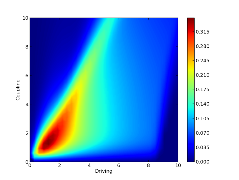
Figure 9: Log negativity as a function of driving field and atom-field coupling for $\kappa=1$ and $\gamma=0.1$.

Note that we have not set $\gamma=0$ as in the work of Alsing et. al. Alsing et al. (1992); Alsing and Carmichael (1991). The phase transition seems to be present as long as $\gamma$ is the smallest rate in the problem.

VII Conclusion

We have investigated entanglement in an open quantum system by calculating the log negativity of a system treated via quantum trajectory theory. We believe that this methodology is useful in describing the behavior of entanglement in open systems. We stress that a different unraveling of the master equation via different choices for $\mathcal{S}$ will result in different results. We have found that there is an optimum value of the driving field for generating entanglement. This value is at or below the value at which the atomic inversion begins to saturate. At higher field values, the atom begins to uncouple from the field mode. This decoupling is due to spontaneous emission, which is maximized when the atom is saturated. We have shown that a steady state entanglement is well defined in the ensemble average over trajectories, and that the entangement typically exhibits a larger value transiently than it does in steady state. Additionally, we find that for large driving fields there are detunings for which multi-photon resonances occur. Here, we find behavior similar to that of a two level system. As the driving field is raised to the value $2\epsilon=g$, there is a phase transition to a bimodal regime. We find that near the phase transition atom-field entanglement is appreciable, and is maintained into the bimodal regime where its maximal value is obtained.

The authors would like to thank H. J. Carmichael and J. P. Clemens for extremely useful discussions.

References

- Nielsen and Chuang (2000) M. A. Nielsen and I. L. Chuang, Quantum Computation and Quantum Information (Cambridge University Press, Cambridge, 2000).
- Jaeger (2007) G. Jaeger, Quantum Information: An Overview (Springer, 2007).
- Hill and Wootters (1997) S. Hill and W. K. Wootters, Phys. Rev. Lett. 78, 5022 (1997).
- Wootters (1998) W. K. Wootters, Phys. Rev. Lett. 80, 2245 (1998).
- Vidal and Werner (2002) G. Vidal and R. F. Werner, Phys. Rev. A 65, 032314 (2002).
- Greenberger (1990) D. M. Greenberger, American Journal of Physics 58, 11131 (1990).
- Dür et al. (2000) W. Dür, G. Vidal, and J. I. Cirac, Phys. Rev. A 62, 062314 (2000).
- Coffman et al. (2000) V. Coffman, J. Kundu, and W. K. Wooters, Phys. Rev. A 61, 052306 (2000).
- Horodecki et al. (2009) R. Horodecki, P. Horodecki, M. Horodecki, and K. Horodecki, Rev. Mod. Phys. 81, 865 (2009).
- Nha and Carmichael (2004) H. Nha and H. J. Carmichael, Phys. Rev. Lett. 93, 120408 (2004).
- Carmichael (1993) H. J. Carmichael, An Open Systems Approach to Quantum Optics, Lecture Notes in Physics, New Series: Monographs, Vol. m18 (Springer, Berlin, 1993).
- Mølmer and Castin (1996) K. Mølmer and Y. Castin, Quantum and Semiclassical Optics: Journal of the European Optical Society Part B 8, 49 (1996).
- Tian and Carmichael (1992) L. Tian and H. J. Carmichael, Phys. Rev. A 46, R6801 (1992).
- Wiseman (1996) H. M. Wiseman, Quantum and Semiclassical Optics: Journal of the European Optical Society Part B 8, 205 (1996).
- Jacobs and Steck (2006) K. Jacobs and D. A. Steck, Contemporary Physics 47, 279 (2006).
- Guevara and Viviescas (2014) I. Guevara and C. Viviescas, Phys. Rev. A 90, 012338 (2014).
- Johansson et al. (2012) J. R. Johansson, P. D. Nation, and F. Nori, Comp. Phys. Comm. 183, 1760 (2012).
- Johansson et al. (2013) J. R. Johansson, P. D. Nation, and F. Nori, Comp. Phys. Comm. 184, 1234 (2013).
- Carmichael et al. (1991) H. J. Carmichael, R. J. Brecha, and P. R. Rice, Opt. Commun. 82, 73 (1991).
- Brecha et al. (1999) R. J. Brecha, P. R. Rice, and M. Xiao, Phys. Rev. A 59, 2392 (1999).
- Bonifacio and Lugiato (1978) R. Bonifacio and L. A. Lugiato, Phys. Rev. Lett. 40, 1023 (1978).
- Shamailov et al. (2010) S. Shamailov, A. Parkins, M. Collett, and H. Carmichael, Optics Communications 283, 766 (2010).
- Alsing and Carmichael (1991) P. Alsing and H. J. Carmichael, Quantum Optics: Journal of the European Optical Society Part B 3, 13 (1991).
- Alsing et al. (1992) P. Alsing, D.-S. Guo, and H. J. Carmichael, Phys. Rev. A 45, 5135 (1992).
- Carmichael (2015) H. J. Carmichael, Phys. Rev. X 5, 031028 (2015).
- Gea-Banacloche et al. (2005) J. Gea-Banacloche, T. C. Burt, P. R. Rice, and L. A. Orozco, Phys. Rev. Lett. 94, 053603 (2005).