Muon $g-2$ through a flavor structure on soft SUSY terms

Abstract

In this work we analyze the possibility to explain the muon anomalous magnetic moment discrepancy within theory and experiment through lepton flavor violation processes. We propose a flavor extended MSSM by considering a hierarchical family structure for the trilinear scalar Soft-Supersymmetric terms of the Lagrangian, present at the SUSY breaking scale. We obtain analytical results for the rotation mass matrix, with the consequence of having non-universal slepton masses and the possibility of leptonic flavour mixing. The one-loop supersymmetric contributions to the leptonic flavour violating process $\tau\to\mu\gamma$ are calculated in the physical basis, instead of using the well known Mass Insertion Method. The flavor violating processes $BR(l_{i}\to l_{j}\gamma)$ are also obtained, in particular $\tau\to\mu\gamma$ is well within the experimental bounds. We present the regions in parameter space where the muon g-2 problem is either entirely solved or partially reduced through the contribution of these flavor violating processes.

¹ FCFM, Universidad Autónoma de Nuevo León, UANL. Ciudad Universitaria, San Nicolás de los Garza, Nuevo León, 66450, Mexico
² DAFM, Universidad de las Américas Puebla, UDLAP. Ex-Hacienda Sta. Catarina Mártir, Cholula, Puebla, Mexico.
³ Instituto de Física, Universidad Nacional Autónoma de México Apdo. Postal 20-364, México 01000 D.F., México.

1 Introduction

It is well known that in contrast to electric charge conservation, lepton number conservation is not associated with a gauge symmetry. In the Standard Model (SM), the spontaneous breaking of the electroweak symmetry produces eigenstates of the remaining gauge group that are not in general eigenstates of the mass matrix [1, 2, 3, 4]. But after diagonalization of the mass matrix, the electroweak coupling matrix is also diagonal in the mass basis, therefore there is no possibility for lepton flavor violation. Certainly this is now in contradiction with the experimental evidence on neutrino mixing [5, 6, 7, 8] and also the possible LFV Higgs decay [9] which forces the structure of the models beyond the SM.

The original structure of the SM with massless, and thus degenerate neutrinos, implied separately $\tau,\mu,e$ number conservation. In particular, the processes $\tau^{\pm}\to l^{\pm}\gamma,(l=\mu^{\pm},e^{\pm})$ through gauge bosons loops are predicted to give very low rates [10], even considering the experimental evidence on neutrino oscillations [5, 6, 7, 8]. Under this evidence the amplitudes for the Lepton Flavor Violation (LFV) processes at low energy are suppressed by an inverse power of the large Majorana mass scale $M_{I}$ used in the well-known seesaw model [11, 12], which explains naturally the small masses for the active left-handed neutrinos. On the other hand, the experimental bounds for the branching ratio $\mathcal{BR}(\tau^{\pm}\to\mu^{\pm}\gamma)$ [13] set strong restrictions on models of physics beyond the SM.

A realistic possibility of physics beyond the SM is offered by supersymmetry (SUSY), whose simplest realization containing the SM is the Minimal Supersymmetric Standard Model (MSSM) (see for instance [14]). In terms of supersymmetry, the SM is embedded in a larger symmetry which relates the fermionic with the bosonic degrees of freedom. As a consequence of this higher symmetry, the SUSY framework stabilizes the electroweak scale, provides us with dark matter candidates, as well as with a greater possibility of unification of all fundamental interactions and a solution to the hierarchy problem.

The discovery of the Higgs boson [15, 16, 17, 18] and the search for sparticles at the LHC, have modified the parameter space of supersymmetry as a near electroweak (EW) scale model [19, 20, 21, 22]. The MSSM, as the first minimal supersymmetric extension of the SM, was conceived to be near to the electroweak scale, in order to set viable phenomenological scenarios to analyze with available experimental data. One important issue to be considered was the experimental absence of Flavor Changing Neutral Currents (FCNC), which lead to the simplifying assumption of universality in the sfermion scalar masses, keeping the desired good behavior of FCNC’s (i.e. bounded) and in addition, reducing the number of free parameters.

The Constrained Minimal Supersymmetric Standard Model (CMSSM) was conceived under the assumption of Grand Unified Theories (GUT) structures. It considers in particular universal sfermion masses and alignment of the trilinear soft scalar terms, $A_{f,ij}$ to Yukawa couplings at the unification scale [23, 24]. Nevertheless, neutrino oscillations made it imperative to reconsider the flavour structure in the theoretical models.

The most recent LHC data points to a heavy spectrum for some of the SUSY particles in the case this constrained model were realized in nature. The relation between the Higgs mass and the fermions and sfermions masses in supersymmetric models indicate either higher stops masses or large mixture within stops [25]. It is the squark sector, and particularly the stop and gluino, which tend to lift the mass scale of the MSSM [26, 20, 21, 22, 27]. However, for the slepton sector the LHC data for the exclusion bounds are less restrictive and masses may still be below the TeV scale [28].. On the other hand, we could go beyond the constrained MSSM and explore other possibilities for the flavor structure. It is thus very relevant to search for SUSY effects to indirect electroweak precision processes through quantum corrections involving superparticles, as the phenomenologically viable parameter space is modified by experimental data, being this the main motivation of the present work.

In the MSSM the conventional mechanism to introduce LFV is through the Yukawa couplings of the right handed neutrinos, $N_{i}$, which generate off-diagonal entries in the mass matrices for sleptons through renormalization effects [29, 30], particularly in the $LL$ block. Then the predicted rates for the $\tau\to\mu\gamma$ and $\mu\to e\gamma$ decays are not suppressed, and depend on the unknown Yukawa matrix elements, but they will not be detected in the future experiments if those elements are too small.

In Ref. [31] the authors work also with these LFV processes, using the seesaw mechanism in the SM [32] and supersymmetric models to extended neutrino and sneutrino sectors, and perform the one-loop calculation through the Renormalization Group Equations (RGEs) based on leading-log approximation. In the SM they use the neutrino-gauge loops, while in the supersymmetric model they get the sneutrino-chargino loops.

In Ref. [33] the authors noticed that there is another source of LFV, namely the left-right mixing terms in the slepton mass matrix, and that their contributions to the LFV processes can be large even when the off diagonal Yukawa couplings elements are small. Later, in a second paper[34], they incorporated the full mixing of the slepton masses and mixing in the neutralino and chargino sector and then performed a numerical diagonalization of the slepton mass matrices. An interesting result of their analysis is that the contribution from the left-right mixing is only important in the region where the mixing term is $m_{\tau}\mu\tan\beta\sim\mathcal{O}(\tilde{m}^{2}_{S})$ and they consider the trilinear soft terms $A_{E,ij}$ contribution negligible. In the above expression $m_{\tau}$ is the tau mass, $\mu$ ($\mu_{susy}$ throughout this paper) is the Higgsino mass parameter; $\tan\beta=v_{2}/v_{1}$ is the ratio of Higgs vacuum expectation values (vevs) and $\tilde{m}^{2}_{S}$ is the supersymmetric scalar mass scale from the soft SUSY breaking. It is worth noting, though, that this analysis was done with very different considerations on experimental data than those we have now.

A more recent work on this relation between the seesaw mechanism for neutrino mixing and charged lepton flavor violation is done in Ref. [35], where a non-trivial neutrino Yukawa matrix at the GUT scale leads to non-vanishing LFV interactions at the seesaw scale through the RGEs. Another approach to the same problem has been done using high-scale supersymmetry in Ref. [36], where the Majorana mass matrix of right-handed neutrinos is taken to be diagonal and universal, while the neutrino Yukawa matrix is proportional to the neutrino Pontecorvo-Maki-Nakagawa-Sakata (PMNS) mixing matrix $U_{PMNS}$, and the product of the left and right handed neutrino masses is $y_{\nu,Ij}=\frac{\sqrt{2M_{N_{R}}m_{\nu_{L,I}}}[U_{PMNS}]_{Ij}}{v\sin\beta}$.

This neutrino Yukawa matrix, which would be present in low energy phenomenology, changes also with the RGE running of the soft SUSY breaking parameters. This scheme of FV was proposed in Ref. [37], where small off-diagonal elements of the slepton mass matrix are considered and, in the interaction basis, the FV processes are restricted by using these off-diagonal elements as free parameters; here the trilinear coupling is considered to be zero, $A=0$. In Ref. [38] the trilinear coupling $A_{0}$ is considered only for the LR flavor mixing term, in the LR term of the corresponding slepton $A_{0}$ is set it to zero. There is also a more general phenomenological work considering non-diagonal LL, RR and EL blocks of sfermion mass matrices which are parameterized as a sfermion mass product and a free parameter for each matrix element in order to do a numerical evaluation of the processes in the mass basis [39], having all the elements of the $6\times 6$ sfermion mass matrix as parameters that might be constrained by the LFV processes. Recent analysis of these general FV contributions are done in [40, 41]. This general sfermion mass matrix, although complete, implies a considerable increase in the number of parameters. Nevertheless, the authors found in seven different possible scenarios an upper bound for their off-diagonal parameter. We must say here that in most of the literature, although the calculation is done in a physical basis, what is done is a diagonalization of $2\times 2$ blocks flavor sleptons and they still consider a flavour mixing parameter, which is off-diagonal on the mass matrix and is used as coupling in the MIA method, so their physical basis means that instead of using the interaction basis states $\tilde{l}_{i,L},\tilde{l}_{i,R}$, they use $\tilde{l}_{i,1},\tilde{l}_{i,2}$ with $i=1,2,3$ as flavors.

There is as well work on supersymmetric models where $R-parity$ violation is considered in the allowed superpotential operators [42], with the consequence of having LFV couplings directly present in the model.

A very important issue to be considered when lepton flavor mixing is allowed is the extra contribution to the anomalous magnetic moment of the muon. The experimental value of the $g-2$ is another element of the electroweak (EW) precision data which has not been completely explained by the SM [43, 44, 45], despite the efforts that have been made for improving the hadronic contribution calculations [46, 47, 48], the dominant source of uncertainty in the theoretical prediction. It is well known that the main MSSM contribution to $g-2$ (we will call it $a_{\mu}$), involves neutralino-slepton and chargino-sneutrino loops [37, 49]. Even the two-loop contribution in terms of $\tan\beta$ has been calculated in Ref. [50], where a reduction was found of the discrepancy coming from an extra contribution, within $14\%$ to $6\%$ of the one-loop MSSM contribution, depending on different scenarios of parameter space.

In Ref. [51] the supersymmetric calculation of $a_{\mu}$ has been updated considering both the chargino-sneutrino loop and the neutralino-smuon loop. It was found that the chargino-sneutrino loop dominates, especially in the case where all the scalar masses are degenerate and, on the other hand, when the $\mu_{susy}$ parameter is large, then $\tilde{\chi}^{0}-\tilde{\mu}$ could be enhanced. There has also been work done relating the parameters for g-2 anomaly, flavour violation, and $h\to\gamma\gamma$ in [52].

In this work we present an analysis of a flavor violating extension of the MSSM (FV-MSSM) one-loop contribution to $a_{\mu}$, which is driven by a LFV mechanism at tree level. The LFV process $\tau\to\mu\gamma$ is used as an additional constraint of the parameter space of the FV-MSSM. Our strategy for the implementation of LFV consists in assuming that $A_{E,ij}$-terms follow a particular structure in the context of textures. Furthermore, we take an ansatz for the mass matrix for sleptons, allowing an exact diagonalization [53] that results in a non-universal spectra for sfermion masses, providing a clear way for having flavour mixing within sleptons at tree level and the opportunity to work in the mass eigenstates basis. Concerning the extra contribution to the anomaly coming from the FV-MSSM, we assume that it comes mainly from the slepton-bino loop, $a_{\mu}^{\tilde{l}\tilde{B}}$, and we compare with the usual MSSM contribution from this loop.

The paper is organized as follows: In Sect. 2 we present the flavor structure of sleptons from an ansatz for the trilinear scalar terms. Then in Sect. 3 we show the one-loop analytical calculation of $BR(\tau\to\mu\gamma)$. In Sect. 4 we include the $a_{\mu}$ calculation and present the combined results in Sect. 5. Finally, we discuss our conclusions in Sect. 6.

2 Flavor structure in the soft SUSY breaking Lagrangian

If supersymmetry exists in Nature it has to be broken, since there is no evidence that these new particles exist at low energies [19]. This symmetry breaking is achieved by the introduction of terms in the Lagrangian, which break SUSY in such a way as to decouple the SUSY partners from the SM particles, and at the same time stabilize the Higgs boson mass to solve the hierarchy problem (see for instance [23]). The soft SUSY breaking Lagrangian in general includes trilinear scalar couplings $A_{ij}^{H}$, as well as bilinear couplings $B_{ij}$, scalar squared mass terms $\tilde{M}^{2}_{\tilde{f}}$, and mass terms for the gauginos $M^{2}_{i}$.

Specifically, for the scalar fermion part of the soft SUSY terms in absence of flavor mixing, as is considered in the MSSM, it will have the following structure:

$$\mathcal{L}_{soft}^{f}=-\sum_{\tilde{f}_{i}}\tilde{M}_{\tilde{f}}^{2}\tilde{\bar{f}}_{i}\tilde{f}_{i}-(A_{\tilde{f},i}\tilde{\bar{f_{L}}}^{i}H_{1}\tilde{f_{R}}^{i}+h.c),$$ (1)

where $\tilde{f}$ are the scalar fields in the supermultiplet. In the case of sfermions the $L,R$ are just labels which point out to the fermionic SM partners, but as we are dealing with scalar fields they have no longer left and right $SU(2)$ properties. In general they may mix in two physical states by means of a $2\times 2$ rotation matrix,

$$\begin{pmatrix}\tilde{f}_{L}\\ \tilde{f}_{R}\end{pmatrix}\leftrightarrow\begin{pmatrix}\tilde{f}_{1}\\ \tilde{f}_{2}\end{pmatrix}\leavevmode\nobreak\ .$$

The first terms in (1) contribute to the diagonal terms of the $2\times 2$ sfermion mass matrix, while the second ones are Higgs couplings with the different sfermions, and they contribute to the off-diagonal $L-R$ terms of the mass matrix once the EW symmetry is spontaneously broken. As $i$ is a flavour index we can see that Eq. (1) implies no flavor mixing.

In our case, where we do consider flavour mixing in the trilinear terms, $A_{f}^{ij}$ would be a general $3\times 3$ matrix, since we consider together the three flavours, with two scalar fields for each one. The complete fermionic trilinear terms are given as

$$\mathcal{L}^{soft}_{H\tilde{f}_{i}\tilde{f}_{j}}=-A_{u}^{ij}\widetilde{\bar{Q}}_{i}H_{2}\widetilde{U}_{j}-A_{d}^{ij}\widetilde{\bar{Q}}_{i}H_{1}\widetilde{D}_{j}-A_{l}^{ij}\widetilde{\bar{L}}_{i}H_{1}\widetilde{E}_{j}+c.c.$$ (2)

Here $\widetilde{Q}_{i}$ is the squark doublet partner of the SM $SU(2)$ left doublet and $\widetilde{U}_{j},\widetilde{D}_{j}$ are the corresponding squarks singlets, while $\widetilde{\bar{L}}_{i}$ is the slepton doublet and $\widetilde{E}_{j}$ is the singlet. In this work in particular, we only analyze the sleptonic part. We will explain further in this paper the ansatz flavour structure we consider for this. Once the EW symmetry breaking is considered, the above Lagrangian (2) for the sleptonic sector takes the form

$$\mathcal{L}_{H\tilde{f}_{i}\tilde{f}_{j}}=\frac{A_{l}^{ij}}{\sqrt{2}}\left[(\phi_{1}^{0}-i\chi_{1}^{0})\tilde{l}_{iR}^{*}\tilde{l}_{jL}-\sqrt{2}\phi_{1}^{-}\widetilde{l}_{iR}^{*}\widetilde{\nu}_{jL}+v_{1}\tilde{l}_{R}^{*}\tilde{l}_{L}\right]+h.c.$$

The soft terms are not the only contributions to the sfermion mass elements, the supersymmetric auxiliary fields $F$ and $D$ coming from the superpotential also contribute to this mass matrix as we explain in the next section.

2.1 Mass matrix for sfermions

The contribution to the elements of the sfermion mass matrix come from the interaction of the Higgs scalars with the sfermions, which appear in different terms of the superpotential and soft-SUSY breaking terms as is fully explained in [54, 55]. In the case of the slepton mass matrix, as we said before, the contributions coming from mass soft terms are $\tilde{M}_{l,LL}^{2}$, $\tilde{M}_{l,RR}^{2}$, from trilinear couplings after EW symmetry breaking $A_{ij}^{l}$ and from the $F,D-$terms. We arrange them in a block mass matrix as follows:

$$\tilde{M}_{l}^{2}=\begin{pmatrix}\tilde{M}_{l,LL}^{2}+F_{l,LL}+D_{l,LL}&A_{ij}^{l}+F_{l,LR}\\ (A_{ij}^{l}+F_{l,LR})^{\dagger}&\tilde{M}_{l,RR}^{2}+F_{l,RR}+D_{l,RR}\leavevmode\nobreak\ \end{pmatrix}\leavevmode\nobreak\ .$$ (3)

The $F_{f}$ and $D_{f}$ are the auxiliary fields in the supermultiplets, which are introduced to have the same bosonic and fermionic degrees of freedom, but are dynamical spurious [14]. The $F$-auxiliary field comes from the Higgs chiral superfields and contributes to the mass matrix as follows:

$$F_{l,LL,RR} = m_{l}^{2}(\tilde{\bar{l}}_{L}\tilde{l}_{L}+\tilde{\bar{l}}_{R}\tilde{l}_{R})$$

$$F_{l,LR} = m_{l}\mu_{susy}\tan\beta(\tilde{l}_{R}^{*}\tilde{l}_{L}+\tilde{l}_{L}^{*}\tilde{l}_{R})$$ (4)

From the $D-$auxiliary fields which come from the scalar superfields of fermions we have the following mass terms:

$$D_{l,LL,RR}=-M_{Z}^{2}\cos 2\beta[(T_{3l}-s_{W}^{2}Q_{l})\tilde{\bar{l}}_{L}\tilde{l}_{L}+s_{W}^{2}Q_{l}\tilde{\bar{l}}_{R}\tilde{l}_{R}]$$ (5)

where $l=e,\mu,\tau$. The elements of the sleptons mass matrix Eq. (3), for the different flavors given by $i,j=e,\mu,\tau$ are

$$m_{LL,l}^{2} = \tilde{M}_{\tilde{L,l}}^{2}+m_{l_{L}}^{2}+\frac{1}{2}\cos 2\beta(2M_{W}^{2}-M_{Z}^{2}),$$ (6)

$$m_{RR,l}^{2} = \tilde{M}_{\tilde{E},l}^{2}+m_{l_{R}}^{2}-\cos 2\beta\sin^{2}\theta_{W}M_{Z}^{2},$$ (7)

$$m_{LR,l}^{2} = \frac{A_{l}v\cos\beta}{\sqrt{2}}-m_{l}\mu_{susy}\tan\beta.$$ (8)

2.2 Soft trilinear terms ansatz

The lepton-flavor conservation is easily violated by taking non-vanishing off-diagonal elements for each matrix, the size of such elements is strongly constrained from the experiments. In the CMSSM, it is assumed that the soft sfermion $2\times 2$ mass matrices $\tilde{m}_{E}^{2},\tilde{m}_{L}^{2}$ are proportional to the identity matrix, and $A_{e,ij}$ is proportional to the Yukawa matrix $y_{e,ij}$. With these soft terms the lepton-flavor number is conserved exactly [33]. The non-universality of scalar masses has been studied in supersymmetric models in the context of string theory [56]. In Ref. [57], the authors assume a non-universality of scalar masses, through off-diagonal trilinear couplings at higher energies. In Refs. [58, 59] a SU(3) flavor symmetry is introduced, then by means of the Froggat-Nielsen mechanism the associated flavon fields acquire vevs, which upon spontaneous symmetry breaking generate the couplings which mix flavours.

In the present work, we assume $\tilde{m}_{RR,l}^{2}\approx\tilde{m}_{LL,l}^{2}=\tilde{m}_{S}^{2}$ but we propose that there is a mixing of two of the scalar lepton families in the $LR$ mass terms. This mixing may come from a discrete flavor symmetry, as could be the extension of the SM with $S_{3}$ [60, 61, 62], or supersymmetric models with $Q_{6}$ [63, 64, 65, 66], which have the fermions assigned to doublet and a third family in a singlet irreducible representations. In order to analyze the consequences of this flavor structure we construct an ansatz for the trilinear terms $A_{t}$. Our procedure is similar to the work done in Ref. [67] for FCNC’s in the quark sector through an ansatz of soft-SUSY terms. In our case we consider the whole two families contributions and of the same order of magnitude, having the following form for the trilinear term:

$$A_{l}=\begin{pmatrix}0&0&0\\ 0&w&y\\ 0&y&1\end{pmatrix}A_{0}.$$ (9)

In this case one could have at tree level the selectrons in a singlet irrep., decoupled from the other two families of sleptons. This would give rise to a $4\times 4$ matrix, diagonalizable through a unitary matrix $Z_{\tilde{l}}$, such that $Z_{\tilde{l}}^{{\dagger}}\tilde{M}_{l}^{2}Z_{\tilde{l}}=\tilde{M}_{diag}^{2}$.

Since we assumed that the mixing is in the smuons and staus only and the selectrons are decoupled, the remaining $4\times 4$ smuon-stau mass matrix will have the following form:

$$\tilde{M}_{\mu-\tau}^{2}=\left(\begin{array}[]{cccc}m_{LL,\mu}^{2}&X_{m}&0&A_{y}\\ X_{m}&m_{RR,\mu}^{2}&A_{y}&0\\ 0&A_{y}&m_{LL,\tau}^{2}&X_{t}\\ A_{y}&0&X_{t}&m_{RR,\tau}^{2}\end{array}\right),$$ (10)

where

$$A_{y} =\frac{1}{\sqrt{2}}yA_{0}v\cos\beta,$$

$$X_{m} =\frac{1}{\sqrt{2}}wA_{0}v\cos\beta-\mu_{susy}m_{\mu}\tan\beta,$$

$$X_{t} =\frac{1}{\sqrt{2}}A_{0}v\cos\beta-\mu_{susy}m_{\tau}\tan\beta.$$ (11)

This way we will have physical non-degenerate slepton masses.

$$m^{2}_{\tilde{\tau}_{1,2}} = \frac{1}{2}(2\tilde{m}_{S}^{2}-X_{m}-X_{t}\pm R)$$

$$m^{2}_{\tilde{\mu}_{1,2}} = \frac{1}{2}(2\tilde{m}_{S}^{2}+X_{m}+X_{t}\pm R)$$ (12)

where $R=\sqrt{4A_{y}^{2}+\left(X_{t}-X_{m}\right)^{2}}$

We may write the transformation which diagonalizes the mass matrix as in Ref.[53], as a $4\times 4$ rotation matrix for sleptons $Z_{\tilde{l}}$, which is in turn a $2\times 2$ block matrix $Z_{\tilde{l}}^{{\dagger}}\tilde{M}_{\mu-\tau}^{2}Z_{\tilde{l}}=\tilde{M}_{l,diag}^{2}$, explicitly having the form

$$Z_{\tilde{l}}=\frac{1}{\sqrt{2}}\left(\begin{array}[]{cc}\Phi&-\Phi\\ \Phi\sigma^{3}&\Phi\sigma^{3}\end{array}\right)\leavevmode\nobreak\ ,$$ (13)

where $\sigma_{3}$ is the Pauli matrix and

$$\Phi=\left(\begin{array}[]{cc}-\sin\frac{\varphi}{2}&-\cos\frac{\varphi}{2}\\ \cos\frac{\varphi}{2}&-\sin\frac{\varphi}{2}\end{array}\right).$$ (14)

The non-physical states are transformed to the physical eigenstates by

$$\begin{pmatrix}\tilde{\mu}_{L}\\ \tilde{\tau}_{L}\\ \tilde{\mu}_{R}\\ \tilde{\tau}_{R}\end{pmatrix}=\frac{1}{\sqrt{2}}\left(\begin{array}[]{cccc}-\sin\frac{\varphi}{2}&-\cos\frac{\varphi}{2}&\sin\frac{\varphi}{2}&\cos\frac{\varphi}{2}\\ \cos\frac{\varphi}{2}&-\sin\frac{\varphi}{2}&-\cos\frac{\varphi}{2}&\sin\frac{\varphi}{2}\\ -\sin\frac{\varphi}{2}&\cos\frac{\varphi}{2}&-\sin\frac{\varphi}{2}&\cos\frac{\varphi}{2}\\ \cos\frac{\varphi}{2}&\sin\frac{\varphi}{2}&\cos\frac{\varphi}{2}&\sin\frac{\varphi}{2}\\ \end{array}\right)\begin{pmatrix}\tilde{l}_{1}\\ \tilde{l}_{2}\\ \tilde{l}_{3}\\ \tilde{l}_{4}\end{pmatrix}=Z_{\tilde{l}}\begin{pmatrix}\tilde{\mu}_{1}\\ \tilde{\tau}_{1}\\ \tilde{\mu}_{2}\\ \tilde{\tau}_{2}\end{pmatrix}$$ (15)

where

$$\tan\varphi = \frac{2A_{y}}{X_{m}-X_{t}},$$

In the case of the MSSM without slepton mixing we would need to revert the similarity transformation performed as $Z_{\tilde{l}}\tilde{M}_{l,diag}^{2}(y=0)Z_{\tilde{l}}^{{\dagger}}=M_{\tilde{\mu},\tilde{\tau}}$, vanishing also the mixing parameter, $y=0$. Then we will get a diagonal by blocks matrix, where the two $2\times 2$ bloques are the mass matrix for smuons and staus, respectively which can in turn be diagonalize separately as in the usual MSSM, obtaining the two sleptons physical states $\tilde{l}_{1},\tilde{l}_{2}$ for each flavor that we identify with the MSSM slepton eigenstates. The masses for the smuons would then be the usual ones,

$$m_{\tilde{\mu}_{1,2}}^{2}=\tilde{m}_{S}^{2}-\frac{1}{2}M_{Z}^{2}\cos 2\beta\pm\sqrt{M_{Z}^{2}\cos 2\beta(-\frac{1}{2}+2s_{w}^{2})^{2}+4X}\leavevmode\nobreak\ ,$$ (17)

where $X=A_{0}\frac{v\cos\beta}{\sqrt{2}}-\mu_{susy}\tan\beta m_{\mu}$.

2.3 Neutralino-lepton-slepton interaction

We assume the usual MSSM form of neutralinos as a mixing of the fermionic part of vector superfields, i.e. gauginos and Higgsinos. The symmetric mass matrix for neutralinos is given by

$$M_{N}=\left(\begin{array}[]{c c c c}M_{1}&0&-M_{Z}\sin{\theta_{W}}\cos{\beta}&M_{Z}\sin{\theta_{W}}\sin{\beta}\\ &M_{2}&M_{Z}\cos{\theta_{W}}\cos{\beta}&-M_{Z}\cos{\theta_{W}}\sin{\beta}\\ &*&0&-\mu_{susy}\\ &*&*&0\end{array}\right).$$

The diagonalization of the mass matrix implies transformation of the neutralinos as

$$\left(\begin{array}[]{c}\tilde{\chi}^{0}_{1}\\ \tilde{\chi}^{0}_{2}\\ \tilde{\chi}^{0}_{3}\\ \tilde{\chi}^{0}_{4}\end{array}\right)=\left(\begin{array}[]{cccc}\eta_{1}&0&0&0\\ 0&\eta_{2}&0&0\\ 0&0&\eta_{3}&0\\ 0&0&0&\eta_{4}\end{array}\right)(\Theta_{N})\left(\begin{array}[]{c}\tilde{B}^{0}\\ \tilde{W}^{0}\\ \tilde{H}_{1}^{0}\\ \tilde{H}_{2}^{0}\end{array}\right).$$

In the rotation matrix $\eta$ is a diagonal matrix, whose elements $\eta_{j}$ are introduced in such a way as to change the phase of those neutralinos whose eigenvalues become negative after diagonalization, i.e. $\eta_{j}=1$ for $m_{\chi^{0}_{j}}>0$ and $\eta_{j}=i$ for $m_{\chi^{0}_{j}}<0$.

The general interaction Lagrangian for neutralino-fermion-sfermion in the MSSM is given as follows [54]

$$\mathcal{L}_{\tilde{\chi}^{0}\tilde{f}f} = -\frac{g}{\sqrt{2}}\sum_{n}^{4}\bigg{\{}\sum_{X=1}^{3}\bar{\tilde{\chi}}_{n}^{0}\left[l_{n}^{NfL}P_{L}+r_{n}^{NfL}P_{R}\right]f\tilde{f}_{X}^{*}$$ (18)

$$+\sum_{X=4}^{6}\bar{\tilde{\chi}}_{n}^{0}\left[l_{n}^{NfR}P_{L}+r_{n}^{NfR}P_{R}\right]f\tilde{f}_{X}^{*}\bigg{\}}+h.c.$$

where the $(l_{n})$ and ($r_{n}$) are the left and right fermion-neutralino couplings, respectively. In this expression the $P_{L,R}$ are the ordinary chiral operators, and the labels for the corresponding scalar superpartners of fermions are $L$ for sfermions $X=1,2,3$ and $R$ for $X=4,5,6$ in the interaction basis and $g$ is the $U(1)$ coupling constant.

The neutralino-fermion-sfermion couplings in equation (18) are given by

$$l_{n}^{NeL} = -\eta^{*}_{n}[(\Theta_{N})_{n2}+\frac{s_{W}}{c_{W}}(\Theta_{N})_{n1}]\leavevmode\nobreak\ ,$$ (19)

$$r_{n}^{NeL} = \eta_{n}\frac{m_{e}}{M_{W}\cos{\beta}}(\Theta_{N})_{n3}\leavevmode\nobreak\ ,$$ (20)

$$l_{n}^{NeR} = \eta_{n}^{*}\frac{m_{e}}{M_{W}\cos{\beta}}(\Theta_{N})_{n3}\leavevmode\nobreak\ ,$$ (21)

$$r_{n}^{NeR} = 2\eta_{n}\frac{s_{W}}{c_{W}}(\Theta_{N})_{n1}\leavevmode\nobreak\ ,$$ (22)

where $\eta\Theta_{N}$ is the rotation matrix which diagonalizes the neutralino mass matrix [68].

Now, considering the sleptons mass eigenstates given in (15) we rewrite the neutralino-lepton-slepton interaction Lagrangian as

$$\mathcal{L}_{\tilde{\chi}^{0}\tilde{l}l} = -\frac{g}{\sqrt{2}}\sum_{n}^{4}\bar{\tilde{\chi}}_{n}^{0}\bigg{\{}C_{n+}^{NeLR}\left[\sin\frac{\varphi}{2}(\tau\tilde{\tau}_{2}^{*}-\mu\tilde{\mu}_{1}^{*})+\cos\frac{\varphi}{2}(\mu\tilde{\tau}_{2}^{*}+\tau\tilde{\mu}_{1}^{*})\right]+$$ (23)

$$-C_{n-}^{NeLR}\left[\sin\frac{\varphi}{2}(\tau\tilde{\tau}_{1}^{*}-\mu\tilde{\mu}_{2}^{*})+\cos\frac{\varphi}{2}(\mu\tilde{\tau}_{1}^{*}+\tau\tilde{\mu}_{2}^{*})\right]\bigg{\}}\leavevmode\nobreak\ ,$$

where $C_{n\pm}^{NeLR}=C_{n}^{NeL}\pm C_{n}^{NeR}$ and $C_{n}^{NeL(R)}=l_{n}^{NeL(R)}P_{L}+r_{n}^{NeL(R)}P_{R}$.

So, we can see here that we directly introduce the FV into the interaction Lagrangian avoiding the need of a mass insertion in the propagators of the loops.

3 $BR(\tau\to\mu+\gamma$)

In general, the way lepton flavor violation is introduced in calculations in the supersymmetric loops is using the approximation method called Mass Insertion Approximation (MIA) [69, 70, 71, 39], which uses a Taylor expansion in a mass parameter [72] giving qualitative good results [73]. Then the calculation is done in a non-mass eigenstate basis expanding around the universal squark masses [74]. This method assumes that off-diagonal elements are small, which generates a strong restriction on the allowed SUSY parameters. On the other hand, working in the interaction basis the number of loops to be calculated is reduced to one, giving a simple analytical expression for the free parameters involved. Concerning flavour violation via neutrino and sneutrino mixing, including a right-handed neutrino [33], the MIA method is used to compute the one-loop amplitude for this process.

In this paper, rather than using the MIA method, we work in a physical basis by diagonalizing exactly the complete mass matrix obtaining mixed flavour sleptons, introducing only two free parameters, which we reduce to one by considering $w=1$, assuming the soft trilinear term ansatz proposed in the previous section, Eq. (9).

We now use the couplings obtained to calculate FV processes to establish the feasibility of the ansatz. In particular, we calculate the supersymmetric sfermion-neutralino one-loop contribution to the leptonic flavor violation process $\tau\to\mu+\gamma$, which corresponds to the Feynman diagram given in Fig.1. The experimental bound to the branching ratio for this decay at $90\%$ C.L. [13] is $\mathcal{BR}(\tau^{\pm}\to\mu^{\pm}\gamma)<4.4\times 10^{-8}\leavevmode\nobreak\ .$

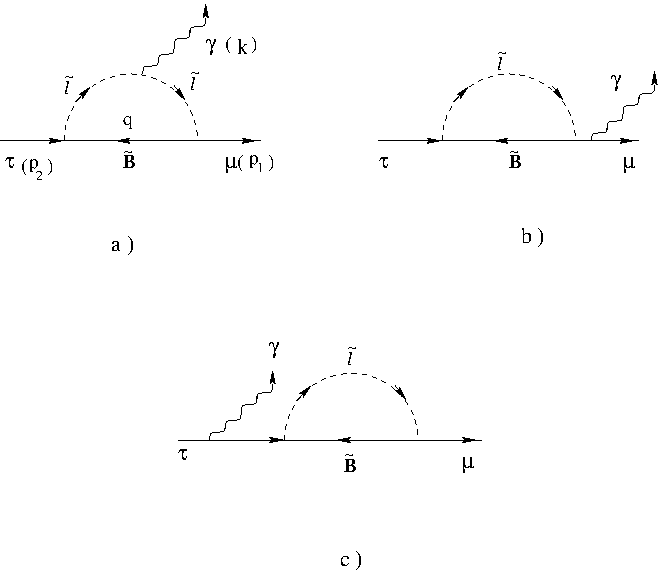
Figure 1: One Loop diagrams in the LFV process $\tau\to\mu\gamma$. The total amplitude is gauge invariant and finite in the UV region.

The loop diagrams shown in Fig.1 are IR safe. A photon is radiated either by a slepton inside the loop or by the external lepton, all three diagrams are needed to achieve gauge invariance. To simplify the expressions, we have assumed that the lightest neutralino is mainly a Bino ($\tilde{B}$), although the procedure can be generalized to any type of neutralino.

Considering the limit $M_{1},M_{2},\mu_{susy}\gg m_{Z}$ [68], then the lightest neutralino is mostly Bino $\tilde{\chi}_{1}^{0}\approx\tilde{B}$ then we take $(\Theta_{N})_{1i}\approx\delta_{1i}$ in Eq. (22). The mass eigenvalue for the lightest neutralino is given by [23]

$$m_{\tilde{N}_{1}}=M_{1}-\frac{m_{Z}^{2}s_{W}^{2}(M_{1}+\mu\sin 2\beta)}{\mu^{2}-M_{1}^{2}}+\cdots$$ (24)

Then this would be a Bino-like neutralino in the limit for numerical values $M_{1}<M_{2}\ll|\mu_{susy}|$. In this case the Bino-lepton-slepton coupling can be written as follows:

$$g_{\tilde{B}l_{i}\tilde{l}}=-\frac{g\tan\theta_{W}}{4}[S_{\tilde{B}l_{i}\tilde{l}}+P_{\tilde{B}l_{i}\tilde{l}}\gamma^{5}]\ ,$$

where $\tilde{l}$ runs over the eigenstates $\tilde{l}_{1,2,3,4}$ given by Eq.(15). For the $\tau\to\mu+\gamma$ decay the scalar and pseudoscalar couplings are given in Table 1.

$\tilde{l}$	$\tilde{\mu}_{1}$	$\tilde{\mu}_{2}$	$\tilde{\tau}_{1}$	$\tilde{\tau}_{2}$
$S_{\tilde{B}\tau\tilde{l}}$	$3\sin\frac{\varphi}{2}$	$\sin\frac{\varphi}{2}$	$\cos\frac{\varphi}{2}$	$3\cos\frac{\varphi}{2}$
$P_{\tilde{B}\tau\tilde{l}}$	$\sin\frac{\varphi}{2}$	$3\sin\frac{\varphi}{2}$	$3\cos\frac{\varphi}{2}$	$\cos\frac{\varphi}{2}$
$S_{\tilde{B}\mu\tilde{l}}$	$3\cos\frac{\varphi}{2}$	$\cos\frac{\varphi}{2}$	$-\sin\frac{\varphi}{2}$	$-3\sin\frac{\varphi}{2}$
$P_{\tilde{B}\mu\tilde{l}}$	$\cos\frac{\varphi}{2}$	$3\cos\frac{\varphi}{2}$	$-3\sin\frac{\varphi}{2}$	$-\sin\frac{\varphi}{2}$

Table 1: Scalar and pseudoscalar Bino-lepton-slepton couplings with lepton flavour mixing

The total amplitude is gauge invariant and free from UV divergences, as it should be, and it can be written in the conventional form,

$$\mathcal{M}_{T}=\bar{u}(p_{1})i\sigma^{\mu\nu}k_{\nu}\epsilon_{\mu}(E+F\gamma^{5})u(p_{2})\ ,$$ (25)

where the one-loop functions $E$ and $F$ contain the sum of the contributions from sleptons $\tilde{l}_{1,2,3,4}$ running inside the loop,

$$E=5C\sum_{\tilde{l}}E_{\tilde{l}}\ ,\qquad F=-3C\sum_{\tilde{l}}F_{\tilde{l}}\ ,\qquad C=\frac{ieg^{2}\tan^{2}\theta_{W}\sin\varphi}{2(16\pi)^{2}(m^{2}_{\tau}-m^{2}_{\mu})}.$$ (26)

The functions $E_{\tilde{l}},F_{\tilde{l}}$ are written in terms of Passarino-Veltman functions and can be evaluated either by LoopTools [75] or by Mathematica using the analytical expressions for $C0$ and $B0$ [76],

$$E_{\tilde{l}} =\frac{\eta(\tilde{l})}{(m_{\tau}+m_{\mu})}\left\{-\left[1+2m^{2}_{\tilde{l}}C0(m^{2}_{\tau},m^{2}_{\mu},0,m^{2}_{\tilde{l}},m^{2}_{\tilde{B}},m^{2}_{\tilde{l}})\right](m^{2}_{\tau}-m^{2}_{\mu})\right.$$

$$\left.+\frac{(m^{2}_{\tilde{l}}-m^{2}_{\tilde{B}})}{x}\left[B0(m^{2}_{\mu},m^{2}_{\tilde{B}},m^{2}_{\tilde{l}})-B0(0,m^{2}_{\tilde{B}},m^{2}_{\tilde{l}})-x^{2}\left[B0(m^{2}_{\tau},m^{2}_{\tilde{B}},m^{2}_{\tilde{l}})-B0(0,m^{2}_{\tilde{B}},m^{2}_{\tilde{l}})\right]\right]\right.$$

$$\left.+\left[B0(m^{2}_{\tau},m^{2}_{\tilde{B}},m^{2}_{\tilde{l}})-B0(m^{2}_{\mu},m^{2}_{\tilde{B}},m^{2}_{\tilde{l}})\right]\left(m_{\tau}m_{\mu}-2(m^{2}_{\tilde{l}}-m^{2}_{\tilde{B}})\right)\right\}$$

$$+(-1)^{r}\frac{8}{5}m_{\tilde{B}}\left[B0(m^{2}_{\tau},m^{2}_{\tilde{B}},m^{2}_{\tilde{l}})-B0(m^{2}_{\mu},m^{2}_{\tilde{B}},m^{2}_{\tilde{l}})\right],$$ (27)

$$F_{\tilde{l}} =\frac{\eta(\tilde{l})}{(m_{\tau}-m_{\mu})}\left\{(m^{2}_{\tau}-m^{2}_{\mu})\left[1+2m^{2}_{\tilde{l}}C0(m^{2}_{\tau},m^{2}_{\mu},0,m^{2}_{\tilde{l}},m^{2}_{\tilde{B}},m^{2}_{\tilde{l}})\right]\right.$$

$$\left.+\frac{(m^{2}_{\tilde{l}}-m^{2}_{\tilde{B}})}{x}\left\{B0(m^{2}_{\mu},m^{2}_{\tilde{B}},m^{2}_{\tilde{l}})-B0(0,m^{2}_{\tilde{B}},m^{2}_{\tilde{l}})-x^{2}\left[B0(m^{2}_{\tau},m^{2}_{\tilde{B}},m^{2}_{\tilde{l}})-B0(0,m^{2}_{\tilde{B}},m^{2}_{\tilde{l}})\right]\right\}\right.$$

$$\left.+\left[B0(m^{2}_{\tau},m^{2}_{\tilde{B}},m^{2}_{\tilde{l}})-B0(m^{2}_{\mu},m^{2}_{\tilde{B}},m^{2}_{\tilde{l}})\right]\left(m_{\tau}m_{\mu}+2(m^{2}_{\tilde{l}}-m^{2}_{\tilde{B}})\right)\right\},$$ (28)

where we have defined the ratio $x=\frac{m_{\mu}}{m_{\tau}}$, and possible values of $r=1,2$ set by $\tilde{l}_{r}$, and the $\eta(\tilde{l})$ function as follows: $\eta(\tilde{\tau}_{1,2})=-1$, $\eta(\tilde{\mu}_{1,2})=1$.

The differential decay width in the $\tau$ rest frame reads

$$d\Gamma=\frac{1}{32\pi^{2}}[\frac{1}{2}\sum|\mathcal{M}|^{2}]\frac{|\vec{p}_{\mu}|d\Omega}{m_{\tau}^{2}}\ ,$$ (29)

where $\vec{p}_{\mu}$ is the 3-vector of the muon. The branching ratio of the $\tau\to\mu+\gamma$ decay is given by the familiar expression,

$$\mathcal{BR}(\tau\to\mu\gamma)=\frac{(1-x^{2})^{3}m^{3}_{\tau}}{4\pi\Gamma_{\tau}}[|E|^{2}+|F|^{2}]\ .$$ (30)

4 The MSSM and the muon anomalous magnetic moment $a_{\mu}$

The anomalous magnetic moment of the muon $a_{\mu}\equiv\frac{g-2}{2}$ is an important issue concerning electroweak precision tests of the SM. The gyromagnetic ratio $g$, whose value $g=2$ is predicted at lowest order by the Dirac equation, will deviate from this value when quantum loop effects are considered. A significant difference between the next to leading order contributions computed within the SM and the experimental measurement would indicate the effects of new physics.

The experimental value for $a_{\mu}$ from the Brookhaven experiment [77] differs from the SM prediction by about three standard deviations. In particular, in Ref.[43] it is found that the discrepancy is

$$\Delta a_{\mu}\equiv a_{\mu}^{Exp}-a_{\mu}^{th}=(287\pm 80)\times 10^{-11},$$ (31)

where $a_{\mu}^{th}$ is the theoretical anomalous magnetic moment of the muon coming only from the SM.

Three generic possible sources of this discrepancy have been pointed out [78]. The first one is the measurement itself, although there is already an effort for measuring $a_{\mu}$ to 0.14 ppp precision [79], and an improvement over this measurement is planned at the J-Parc muon g-2/EDM experiment [80] whose aim is to reach a precision of 0.1 ppm.

The second possible source of discrepancy are the uncertainties in the evaluation of the non-perturbative hadronic corrections that enter in the SM prediction for $a_{\mu}$. The hadronic contribution to $a_{\mu}$ is separated in High Order (HO) and Leading Order (LO) contributions. The hadronic LO is under control, this piece is the dominant hadronic vacuum polarization contribution and can be calculated with a combination of the experimental cross section data involving $e^{+}e^{-}$ annihilation to hadrons and perturbative QCD [48]. The hadronic HO is made of a contribution at ${\cal O}(\alpha^{3})$ of diagrams containing vacuum polarization insertions [81, 82] and the very well known hadronic Light by Light (LbL) contribution, which can only be determined from theory, with many models attempting its evaluation [83, 84]. The main source of the theoretical error for $a_{\mu}$ comes from LO and LbL contributions. It is worth mentioning that the error in LO can be reduced by improving the measurements, whereas the error in LbL depends on the theoretical model.

The third possibility comes from loop corrections from new particles beyond the SM. There have already many analyses been done in this direction (see for instance [33, 85, 86]).

To calculate one-loop effects to g-2, for general contributions coming from different kind of particles Beyond the SM, there is a numerical code built using Mathematica [87].

The supersymmetry contribution to g-2, $a_{\mu}^{SUSY}$, was first computed by Moroi Ref. [37] and recently updated in Ref. [88]. In these works the large $\tan\beta$ scenario was studied, showing the dominance of the chargino-sneutrino loop over the neutralino-smuon loop, provided the scalar masses are degenerate, otherwise the $\mu_{susy}$ parameter (Higgsino mass parameter) must be large allowing an enhancement of the muon-neutralino loop ($\chi^{0}-\tilde{\mu}$). It was also shown that in the interaction basis the dominant contributions are proportional to $\mu_{susy}M_{1}\tan\beta$, then the sign and the size of the contribution to $a_{\mu}^{SUSY}$ depends on the nature of this product. Hence, the supersymmetric contributions to the anomaly are determined by how these elements are assumed (see for instance [37, 88]). The results in the literature are usually obtained using the MIA approximation, however, there are some schemes where the work is done in the physical basis (e.g. [41]). The difference with the MIA method is not only the change in basis, but the restriction that is imposed a priori that some elements in the mass matrix are considered small compared to the diagonal ones.

There has been research toward an MSSM explanation to the $g-2$ discrepancy related to LFV as in [89, 90], since there is a correspondence between the diagrams in the MSSM that contribute to the anomalous magnetic moment of the muon and the diagrams that contribute to LFV processes. The process $\mu\to e+\gamma$ have been used to constrain lepton flavor violation and as a possible connection to $g-2$.

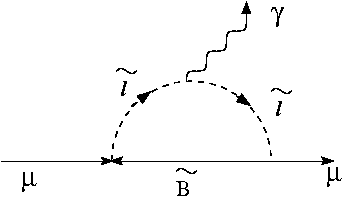
Figure 2: Slepton contribution to $a_{\mu}$.

In this work we assume that there is room for an MSSM contribution to $g-2$ through lepton flavor violation in the sleptonic sector. In particular, we search for the LFV process $\tau\to\mu+\gamma$ and calculate $g-2$ through a mixing of smuon and stau families, $a_{\mu}^{\tilde{l}\tilde{B}}$, Fig. 2. The ansatz proposed here avoids extra $\mu\to e+\gamma$ contributions. To establish the restrictions on parameter space we consider a loose constraint, $|a_{\mu}^{Exp}-a_{\mu}^{TH}|\leq 3.3\sigma$, where $a_{\mu}^{TH}=a_{\mu}^{th}+a_{\mu}^{\tilde{l}\tilde{B}}$ indicates that the lepton flavor violation supersymmetric loop through charged sleptons is not necessarily the only contribution to solve the discrepancy, Eq.(31). We also show the extreme case in parameter space where this loop contribution solves the discrepancy completely $|a_{\mu}^{Exp}-a_{\mu}^{TH}|\leq 1\sigma$.

When taking into account the slepton-bino flavor violation contribution to $g-2$, if the discrepancy is $\leq 1\sigma$, it means that this contribution solves the whole $g-2$ problem. In the opposite scenario, $|a_{\mu}^{Exp}-a_{\mu}^{TH}|\approx 3.3\sigma$ means that the slepton-bino loop gives no significant contribution to the discrepancy. In here we will look at a possible contribution to $g-2$ between both scenarios.

Using the LFV terms constructed previously we obtained the contribution to the anomalous magnetic moment of the muon $a_{\mu}^{\tilde{l}\tilde{B}}$. Defining the ratio $r=m_{\mu}/M_{1}$ and taking the leading terms when $r^{2}\to 0$, and $M_{1}=m_{\tilde{B}}$ as the Bino mass.

In order to compute the SUSY contribution to the $g-2$ anomaly, we follow the method given in Ref.[91]. All we have to do is to isolate the coefficient of the $(p_{1}+p_{2})^{\mu}$ term, in other words, computing the one-loop contribution, we can write the result as follows:

$$\bar{u}(p_{1})\Gamma^{\mu}u(p_{2}) =\bar{u}(p_{1})[B(p_{1}+p_{2})^{\mu}+_{\cdots}]u(p_{2})$$

$$=\bar{u}(p_{1})[\frac{\imath\sigma^{\mu\nu}}{2m_{\mu}}q_{\nu}]F_{2}(q^{2})u(p_{2})+_{\cdots}$$ (32)

where the ellipsis indicates terms that are not proportional to $(p_{1}+p_{2})^{\mu}$. Then the anomaly can be defined as $\delta a_{\mu}=\frac{g-2}{2}=F_{2}(0)$ with $q=p_{2}-p_{1}$.
Keeping in mind that we require the magnetic interaction which is given by the terms in the loop process proportional to $(p_{1}+p_{2})^{\mu}$ we write it as

$$B(p_{1}+p_{2})^{\mu}\ ,$$

$$\frac{g-2}{2} =F_{2}(q^{2}\to 0)=-2m_{\mu}B.$$ (33)

Considering only these terms in the interaction and gathering them, the contribution of the flavour violation loop to the $g-2$ anomaly due to a given slepton $\tilde{l}$ reads

$$\frac{g-2}{2} =\frac{g^{2}_{c}}{(4\pi)^{2}}(S^{2}_{\tilde{B}\mu,\tilde{l}}-P^{2}_{\tilde{B}\mu,\tilde{l}})\frac{2m_{\tilde{B}}m_{\mu}}{\Delta_{\tilde{l}\tilde{B}}}\left[-\frac{1}{2}-\frac{m^{2}_{\tilde{B}}}{\Delta_{\tilde{l}\tilde{B}}}-\frac{m^{2}_{\tilde{B}}m^{2}_{\tilde{l}}}{\Delta_{\tilde{l}\tilde{B}}^{2}}\ln\left[\frac{m^{2}_{\tilde{B}}}{m^{2}_{\tilde{l}}}\right]\right]$$

$$+\frac{g^{2}_{c}}{(4\pi)^{2}}(S^{2}_{\tilde{B}\mu,\tilde{l}}+P^{2}_{\tilde{B}\mu,\tilde{l}})\frac{2m^{2}_{\mu}}{\Delta_{\tilde{l}\tilde{B}}}\left[\frac{1}{6}-\frac{m^{2}_{\tilde{B}}}{2\Delta_{\tilde{l}\tilde{B}}}-\frac{m^{4}_{\tilde{B}}}{\Delta_{\tilde{l}\tilde{B}}^{2}}-\frac{m^{4}_{\tilde{B}}m^{2}_{\tilde{l}}}{\Delta_{\tilde{l}\tilde{B}}^{3}}\ln\left[\frac{m^{2}_{\tilde{B}}}{m^{2}_{\tilde{l}}}\right]\right],$$ (34)

where $g^{2}_{c}=\frac{\rm tan^{2}\theta_{w}g^{2}_{1}}{16}$, and $\Delta_{\tilde{l}\tilde{B}}=m^{2}_{\tilde{l}}-M^{2}_{1}$, having four contributions with $\tilde{l}$ running from 1 to 4 with the values of the couplings $S_{\tilde{B}\mu,\tilde{l}},P_{\tilde{B}\mu,\tilde{l}}$ are given in Table 1.
This expression is equivalent to the one presented in [92] and can be written using their notation as can be found in Appendix B.

The expression will be different from MIA because the off-diagonal elements $LR$ are not explicit since we are in the physical basis. In the interaction basis, the $LR$ terms appear with explicit SUSY free parameter dependence as they use directly the elements of the slepton mass matrix. Exact analytical expressions for the leading one- and two-loop contributions to g-2 in terms of interactions eigenstates can be found in Refs. [49, 92], and references therein. By taking these expressions in the limit of large $\tan\beta$ and of the mass parameters in the smuon, chargino and neutralino mass matrices equal to a common scale $M_{SUSY}$, the results calculated in the mass-insertion approximation in the same limit [37] are reproduced from the complete forms given in [92]. We have explicitly checked that our one-loop results when no LFV terms are present coincide with the analytical expressions of ref. [92], and thus in the appropriate limits also with the MIA expressions. Our expressions for the contribution of the LFV terms to g-2 can be found in Appendix B.

Here we take a flavour structure with no a priori restrictions on the size of the mass matrix elements other than two family mixing, and the restrictions come directly from the comparison with experimental data.

$\mu_{susy}\in[-15,15]$ TeV	$A_{0}\in[50,5000]$ GeV
$\tilde{m}_{S}\in[50,5000]$ GeV	$\frac{M_{1}}{\tilde{m}_{S}}\in[0.2,5]$ GeV
$\tan\beta\in[1,60]$	$w=-1$ , $y=1$

Table 2: The table shows the parameter space where the scan was performed. The values were taken at random for each variable within the bounds shown

.

5 Results

We now analyze the region in parameter space allowed by the experimental bound on $BR(\tau\to\mu\gamma)$, taking into account that the mixing parameters $w,y$ represent at most a phase, i.e. the mixing terms in the $LR$ term of the mass matrix are of the same order as $A_{0}$, see Eq. (9), in contrast with the MIA method where this terms are considered small compared with the diagonal ones which is needed to apply the method. In the parameter space region comprised by Table 2, we are able to safely consider lepton flavour mixing in trilinear soft terms of the MSSM, and constrained it at the current experimental bounds $BR^{exp}(\tau\to\mu\gamma)<4.4\times 10^{-8}\leavevmode\nobreak\$ [93]. Throughout parameter space we take $M_{1}<|\mu_{susy}|$. We highlight the points where the $g-2$ is solved completely, shown in black in all figures. In order to ensure that the lightest neutralino is mostly Bino, we further assume for these points $M_{1}\lesssim\frac{1}{3}|\mu_{susy}|$.

We found for the parameter values given in Table 2 that the $BR(\tau\to\mu\gamma)$ is only partially restricted from experimental bound for $\tilde{m}_{S}\lesssim 3200$ GeV, also for $M_{1}\lesssim 4.5$ TeV. Table 3 shows examples of different sets of values for random parameters given within the range in Table 2, consistent with the experimental bound on LFV and that also solve entirely the g-2 discrepancy, in all these points the Bino is considered as the LSP. From these sets of values it can be seen that the $g-2$ discrepancy can be solved within the FV-MSSM by different possible combinations of the parameters.

The difference between the experimental value and the SM prediction for the anomalous magnetic moment, Eq.(31), gives $\sigma=80\times 10^{-11}$. As we have already explained we distinguish between two possible ways the slepton contribution should be constrained, depending whether the loop is dominant in FV-MSSM or not:

$$0<a_{\mu}^{\tilde{l}\tilde{B}}<6.6\sigma\,\,\,\,$$ any contribution, (35)

$$2.3\sigma<a_{\mu}^{\tilde{l}\tilde{B}}<4.3\sigma\,\,\,\,$$ main contribution. (36)

It is important to mention that we take the points that solve for “any contribution” as defined above (blue in graphs), because we are aware that this is only one of the possible supersymmetric contributions to $g-2$. In a more general case we need to include the chargino-sneutrino contributions in order to have an entire picture of the parameter space. In the FV extension considered here this contribution will be the same as in the usual MSSM. For a more complete treatment right-handed neutrinos should be considered, together with LR mixing and the trilinear term.

$BR(\tau\to\mu\gamma)$	$\alpha_{\mu}^{\tilde{l}\tilde{B}}$	$\tan\beta$	$M_{1}$(GeV)	$\mu_{susy}$(GeV)	$\tilde{m}_{S}$ (GeV)	$A_{0}$(GeV)
$3.06\times 10^{-8}$	$2.17\times 10^{-9}$	$15.4$	$1205$	$7324.6$	$457.6$	$145.2$
$3.01\times 10^{-8}$	$2.06\times 10^{-9}$	$45$	$714$	$10298$	$991$	$1236.7$
$2.33\times 10^{-8}$	$2.42\times 10^{-9}$	$1.35$	$697$	$-2832.2$	$831.8$	$4003.5$
$2.22\times 10^{-8}$	$3.13\times 10^{-9}$	$30.7$	$363.7$	$12554.7$	$832.2$	$340$
$1.22\times 10^{-8}$	$3\times 10^{-9}$	$46.3$	$509.7$	$4681.2$	$691$	$408.5$
$2.06\times 10^{-11}$	$2\times 10^{-9}$	$45.6$	$2064$	$9127$	$1005.7$	$50.7$

Table 3: Sample of parameter sets that solve entirely the muon $g-2$ discrepancy, consistent with the experimental bound on $BR(\tau\to\mu\gamma)$, calculated using random values of the parameters given in Table 2. For all these sets the LSP is a Bino.

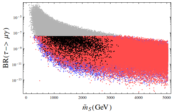
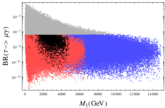
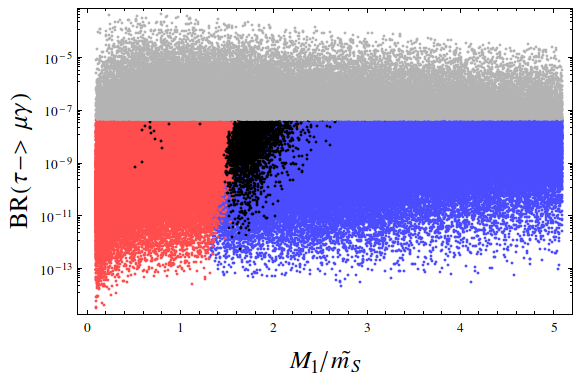
Figure 3: The plots show the dependence on $BR^{theo}(\tau\to\mu\gamma)$ on the SUSY scalar mass $\tilde{m}_{S}$ (left) and the Bino mass $M_{1}$ (right) and on the ratio of them (down). The gray points are excluded by the experimental bound on $BR(\tau\to\mu\gamma)$. The rest of the color code is shown explicit in Fig.4, which separates ranges of FV contributions to $g-2$.

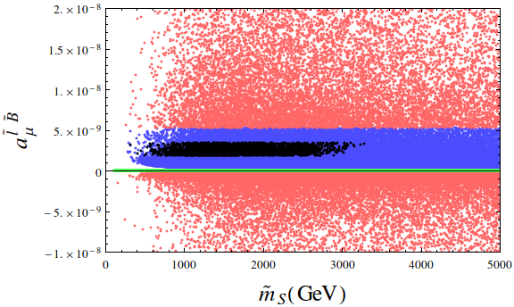
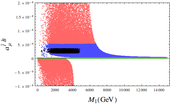
Figure 4: The plots show the dependence of the value of our calculation for $a_{\mu}^{\tilde{l}\tilde{B}}$ with the SUSY scalar mass (left) and the Bino mass (right). Here the color code used in Figs. 3, 5 and 6 is shown explicit as ranges of the $a_{\mu}^{\tilde{l}\tilde{B}}$. The green points correspond to no FV Bino-slepton loop, considering only the smuons in their mass eigenstates and $A_{0}=0$ the same as green points in previous figure (fig. 7).

In Fig. 3 we show the dependence of the $BR(\tau\to\mu\gamma)$ on $\tilde{m}_{S}$ and on the Bino mass $M_{1}$, and it is shown the stringent restrictions for these masses. In Fig. 4 we show the value of $a_{\mu}^{\tilde{l}\tilde{B}}$ for different values of the Bino and the SUSY scalar mass, the color code is clear from this figure. The blue points correspond to the mass scale for which there is any contribution to the discrepancy $a_{\mu}$ Eq. (35). The black ones are those for which the discrepancy would be completely explained by the LFV contribution Eq. (36), for these points we take $M_{1}<\frac{1}{3}|\mu_{susy}|$ (otherwise we just take $M_{1}<|\mu_{susy}|$). The red points are outside these ranges, i.e. are contributions non-compatible with experimental data of the muon g-2 anomaly to be solved. The green points show the results obtained by taking $y=0$ in our ansatz, i.e. no FV, and calculating the smuon-Bino loops for $g-2$ with the smuons masses as given in Eq. (17) and considering a trilinear coupling as $A_{0}=0$.

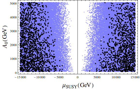
Figure 5: Values of $\tan\beta$ (left) and $A_{0}$ (right) dependence on $\mu_{SUSY}$ for which the $a_{\mu}$ discrepancy would get solved partially by the LFV contributions (blue), or completely up to $1\sigma$ with the restriction $M_{1}<\frac{1}{3}\mu_{susy}$ (black).

Figure  5 shows the relation of $\mu_{susy}$ with $\tan\beta$ and trilinear coupling $A_{0}$ for values for which the $a_{\mu}$ discrepancy receives contributions from the LFV terms. We see that there is a quite symmetrical behavior for any sign of $\mu_{susy}$. In order for the $a_{\mu}$ problem to be solved entirely by LFV $|\mu_{susy}|\gtrsim 4000\leavevmode\nobreak\ GeV$ and no restriction for $\tan\beta$. For smaller values of $A_{0}$ there will be less restriction on $\mu_{susy}$. Although $\mu_{susy}$ values could be restricted by other sectors of the MSSM, e.g. the radiative corrections to the lightest Higgs mass [25, 94]. On the other hand, there are other SUSY models, where the value of $\mu_{susy}$ could be naturally small [95].

Figure  6 shows the ratio of the Bino mass $M_{1}$ with SUSY scalar mass $\tilde{m}_{S}$ where the points showed are solutions to $a_{\mu}$ discrepancy achieved up to $1\sigma$ by the LFV contribution. We see a highly restricted regions for $1.5<M_{1}/\tilde{m}_{S}<2.5$, although we also have few points within $0.4\lesssim M_{1}/\tilde{m}_{S}<0.85$, but there are no points for $0.8\lesssim M_{1}/\tilde{m}_{S}<1.2$. We also see the behavior of these points the scalar mass is highly restricted to the range of values $m_{S}\simeq[500,3400]$ GeV, reaching the top values for larger values of $|\mu_{susy}|$

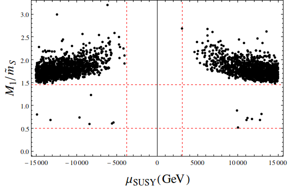
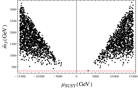
Figure 6: The values for which the LFV contribution would explain completely the $a_{\mu}$ discrepancy within theory and experimental data up to $1\sigma$, considering $M_{1}<\frac{1}{3}\mu_{susy}$. We show ratio on susy mass parameters $M_{1}/\tilde{m}_{S}$ (left) and $\tilde{m}_{S}$ (right), both with respect on $\mu_{susy}$ values.

We consider that in the region of parameter space where the points that solve completely the $g-2$ anomaly lie, the Bino-sleptons loop contribution will dominate over the chargino-sneutrino contribution. Under this consideration is possible that the allowed parameter space is different from the MSSM with no FV terms in the charged lepton sector, where the chargino-sneutrino contribution is the dominant one [96].

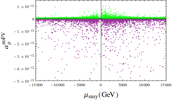
Figure 7: Complete Bino-smuon loop contribution on MSSM with no flavour violation to $g-2$, considering $A_{0}=0$ green points (lighter), and running $A_{0}$ for $(50,5000)\leavevmode\nobreak\ GeV$ purple points (darker).

6 Summary and conclusions

We proposed an ansatz for the trilinear scalar couplings considering a two family flavour structure. We obtain a non-universal slepton spectrum and and slepton states are now flavor mixed. This specific family structure implies the possibility of lepton flavour violation although avoids extra LFV contributions to $BR(\mu\to e\gamma)$. In the method we used the FV is absorbed into the Lagrangian couplings instead of introducing a mass-insertion term into the propagator as used commonly in the literature. This method does not require a priori approximations to reduce the loop amplitude integral expression.

We analyzed the parameter space which gives values for these processes within experimental bounds. We considered that the lightest neutralino is mainly a Bino, specifically we consider the slepton-Bino loops. In order to have the Bino decoupled from Higgsino we take $M_{1}<|mu_{susy}|$. Under these assumptions we showed that this FV couplings will include a mixture of four types of sleptons running in the loop contributing to $a_{\mu}$, which in the interaction basis corresponds to the smuons and the staus, as can be seen in Fig. 2, and that for certain regions of parameter space it is possible to solve entirely the discrepancy between the experimental and theoretical values of $a_{\mu}$, in this case we specifically take a more restricted condition, $M_{1}<1/3|mu_{susy}|$. The points that match with these conditions are given for the scalar SUSY mass scale $\tilde{m}_{S}$ involved in the LFV processes range between $450\lesssim\tilde{m}_{S}<3300$ GeV, the upper bound in the scalar mass is reached for $|\mu_{susy}|\sim 14\leavevmode\nobreak\ TeV$. The possible Bino mass needed in order to solve the $a_{\mu}$ problem ranges from $\sim 350$ GeV to $\sim 7.5$ TeV, nevertheless the ratio of these masses is restricted to $0.4\lesssim\frac{M_{1}}{\tilde{m}_{S}}<3$, although we have very few point for $\frac{M_{1}}{\tilde{m}_{S}}<0.9$, and the points around $\frac{M_{1}}{\tilde{m}_{S}}\sim 1$ are excluded. It is possible to contribute only partially to the $a_{\mu}$ problem, in which case a much larger parameter space is allowed (blue points). This partial contribution to $g-2$ will be important when the chargino-sneutrino contribution is included, since it might change the allowed parameter space. This complete analysis we leave to a forthcoming work. Nevertheless, is worth mentioning again that it is natural to have differences in the parameter space as compared to the usual MSSM, where the chargino-sneutrino contribution is the dominant one.

It is interesting to notice that considering off-diagonal elements in the LR of the mass matrix block to be as large as $\leavevmode\nobreak\ 1$TeV does not necessarily blow up the $BR(\tau\to\mu\gamma)$ process, instead, this assumption helps to reduce partially or completely the $g-2$ discrepancy. In our case, we have considered off-diagonal terms in the soft trilinear couplings, of the order of $50\leavevmode\nobreak\ GeV<A_{0}\lesssim$ 5TeV. We also compare our results with the no flavour violation $g-2$ MSSM one-loop contribution, where we obtain the same expressions given in the literature for complete calculation and in the numerical results we obtain small positive contributions to $g-2$ considering no contribution from the trilinear term $A=0$.

Appendix A Loop amplitude for $\tau\to\mu\gamma$

We present here the expressions we obtain for the invariant amplitude of the processes given in Fig. 1. For clarity in the expressions we have defined $g^{2}_{c}=\frac{\rm tan^{2}\theta_{w}g^{2}_{1}}{16}$. For general leptons in external particles represented by $i,j=e,\mu,\tau$, the diagram in Fig. 1 (a) we have

$$\mathcal{M}_{a} = -eg^{2}_{c}\bar{u}(p_{1})\left[(S_{i}S_{j}-P_{i}P_{j})+(S_{i}P_{j}-S_{j}P_{i})\gamma^{5}\right]m_{\tilde{B}}\frac{1}{(2\pi)^{4}}\int dq^{4}\frac{2(p_{2}+q)\cdot\epsilon}{D_{q}D_{1}D_{2}}$$ (37)

$$-eg^{2}_{c}\bar{u}(p_{1})\left[(S_{i}S_{j}+P_{i}P_{j})+(S_{i}P_{j}+S_{j}P_{i})\gamma^{5}\right]\frac{1}{(2\pi)^{4}}\int dq^{4}\frac{2(p_{2}+q)\cdot\epsilon q\hskip-7.0pt\diagup}{D_{q}D_{1}D_{2}}\ ,$$

where $D_{q}=q^{2}-m^{2}_{\tilde{B}}$, $D_{1}=(q+p_{1})^{2}-m^{2}_{\tilde{l}_{r}}$, $D_{2}=(q+p_{2})^{2}-m^{2}_{\tilde{l}_{r}}$, and $\epsilon$ is the photon polarization vector. For the $\tau\to\mu\gamma$ decay, we have $i=\tau$ and $j=\mu$ and the $S_{i,j}$, $P_{i,j}$ couplings are labeled as follows: $S_{i}=S_{\tilde{B}\tau\tilde{l}}$, $S_{j}=S_{\tilde{B}\mu\tilde{l}}$, $P_{i}=P_{\tilde{B}\tau\tilde{l}}$ and $P_{j}=S_{\tilde{B}\mu\tilde{l}}$. All the possible sleptons running inside the loop are indicated by the index $\tilde{l}=\tilde{\mu}_{1},\tilde{\mu}_{2},\tilde{\tau}_{1},\tilde{\tau}_{2}$. The corresponding values are given in Table 1. For the anomaly $g-2$ we set $i=j=\mu$.
For the diagram Fig. 1(b) we have

$$\mathcal{M}_{b} = -\bar{u}(p_{1})e\Sigma_{b}\frac{[p\hskip-7.0pt\diagup_{1}+m_{i}]}{m^{2}_{j}-m^{2}_{i}}\epsilon\hskip-7.0pt\diagup u(p_{2}),$$ (38)

with

$$\Sigma_{b} = m_{\tilde{B}}g^{2}_{c}\left[(S_{i}S_{j}-P_{i}P_{j})+(S_{i}P_{j}-S_{j}P_{i})\gamma^{5}\right]\frac{1}{(2\pi)^{4}}\int\frac{dq^{4}}{D_{q}D_{1}}$$

$$+g^{2}_{c}\left[(S_{i}S_{j}+P_{i}P_{j})+(S_{i}P_{j}+S_{j}P_{i})\gamma^{5}\right]\frac{1}{(2\pi)^{4}}\int\frac{dq^{4}q\hskip-7.0pt\diagup}{D_{q}D_{1}}.$$

The amplitude for Fig. 1(c) reads

$$\mathcal{M}_{c} = -\bar{u}(p_{1})e\gamma_{\mu}\epsilon^{\mu}\frac{[p\hskip-7.0pt\diagup_{1}+k\hskip-7.0pt\diagup+m_{j}]}{m^{2}_{i}-m^{2}_{j}}\Sigma_{c}u(p_{2}),$$ (40)

where

$$\Sigma_{c} = m_{\tilde{B}}g^{2}_{c}\left[(S_{i}S_{j}-P_{i}P_{j})+(S_{i}P_{j}-S_{j}P_{i})\gamma^{5}\right]\frac{1}{(2\pi)^{4}}\int\frac{dq^{4}}{D_{q}D_{2}}$$

$$+g^{2}_{c}\left[(S_{i}S_{j}+P_{i}P_{j})+(S_{i}P_{j}+S_{j}P_{i})\gamma^{5}\right]\frac{1}{(2\pi)^{4}}\int\frac{dq^{4}q\hskip-7.0pt\diagup}{D_{q}D_{2}}.$$

The total amplitude which is the sum of Eqs.(37, 38, 40) is written as follows:

$$\mathcal{M}_{T} = \bar{u}(p_{1})[\imath E_{ij}\sigma^{\mu\nu}k_{\nu}\epsilon_{\mu}+\imath F_{ij}\sigma^{\mu\nu}k_{\nu}\epsilon_{\mu}\gamma^{5}]u(p_{2})$$ (42)

$$= \bar{u}(p_{1})[\frac{E_{ij}}{2}+\frac{F_{ij}}{2}\gamma^{5}][k\hskip-7.0pt\diagup,\epsilon\hskip-7.0pt\diagup]u(p_{2})\ .$$

In the case of $i=\tau$ and $j=\mu$ we would have the expressions for $E_{ij}$ and $F_{ij}$ as in Eqs.(27, 28).

Appendix B The loop contribution to the muon anomaly

The loop amplitude for the vertex correction is given by

$$\bar{u}(p_{1})\Gamma^{\mu}u(p_{2}) =\imath g_{c}\bar{u}(p_{1})\left[S_{\tilde{B}\mu,\tilde{l}}+P_{\tilde{B}\mu,\tilde{l}}\gamma^{5}\right]\frac{1}{(2\pi)^{4}}\int dk^{4}\frac{\imath[k\hskip-7.0pt\diagup+m_{\tilde{B}}]}{D_{t}}\imath\frac{\rm tan\theta_{w}g_{1}}{4}$$

$$\times[S_{\tilde{B}\mu,\tilde{l}}-P_{\tilde{B}\mu,\tilde{l}}\gamma^{5}]\frac{\imath}{D_{2}}\frac{\imath}{D_{1}}[2k+p_{1}+p_{2}]_{\mu}u(p_{2})$$

$$=\imath g^{2}_{c}\left[S_{\tilde{B}\mu,\tilde{l}}^{2}-P_{\tilde{B}\mu,\tilde{l}}^{2}\right]m_{\tilde{B}}\bar{u}(p_{1})\int\frac{dk^{4}}{(2\pi)^{4}}\frac{(2k+p_{1}+p_{2})^{\mu}}{D_{t}D_{1}D_{2}}u(p_{2})$$

$$+g^{2}_{c}\bar{u}(p_{1})\left[S_{\tilde{B}\mu,\tilde{l}}^{2}+P_{\tilde{B}\mu,\tilde{l}}^{2}\right]\int\frac{dk^{4}}{(2\pi)^{4}}\frac{(2k+p_{1}+p_{2})^{\mu}k\hskip-7.0pt\diagup}{D_{t}D_{1}D_{2}}u(p_{2})+\ldots$$

$$=g^{2}_{c}\bar{u}(p_{1})\left[(S_{\tilde{B}\mu,\tilde{l}}^{2}-P_{\tilde{B}\mu,\tilde{l}}^{2})m_{\tilde{B}}B_{1}^{\mu}(q^{2})\right]u(p_{2})$$

$$+g^{2}_{c}\bar{u}(p_{1})\left[(S_{\tilde{B}\mu,\tilde{l}}^{2}+P_{\tilde{B}\mu,\tilde{l}}^{2})B_{2}^{\mu}(q^{2})\right]u(p_{2})+\ldots,$$ (43)

where $q^{2}=(p_{2}-p_{1})^{2}$ and the ellipsis means terms that are not involved in the determination of the anomaly contribution. The propagators are given by

$$Dt =\frac{1}{k^{2}-m^{2}_{\tilde{B}}}\ ,$$ (44)

$$D_{1} =\frac{1}{(p_{1}+k)^{2}-m^{2}_{\tilde{l}}}\ ,$$ (45)

$$D_{2} =\frac{1}{(p_{2}+k)^{2}-m^{2}_{\tilde{l}}}\ .$$ (46)

By setting $q^{2}=0$ and considering that the muon mass is negligible compared to the supersymmetric particle masses inside the loop, the contributions to the anomaly are found to be

$$B_{1}^{\mu}(0) =(p_{1}+p_{2})^{\mu}(b_{1}+b_{2})\ ,$$ (47)

$$B_{2}^{\mu}(0) =m_{\mu}(p_{1}+p_{2})^{\mu}(b_{2}+b_{4}),$$ (48)

where $m_{\mu}$ is the muon mass and the scalar functions $b_{1,2,4}$ read as

$$b_{1} =-\frac{\imath}{(4\pi)^{2}}\frac{1}{\Delta_{lb}}\left[1+\frac{m^{2}_{\tilde{B}}}{\Delta_{lb}}\ln\left[\frac{m^{2}_{\tilde{B}}}{m^{2}_{\tilde{l}}}\right]\right]\ ,$$ (49)

$$b_{2} =-\frac{\imath}{(4\pi)^{2}}\frac{1}{\Delta_{lb}}\left[-\frac{1}{2}+\frac{m^{2}_{\tilde{B}}}{\Delta_{lb}}-\frac{m^{4}_{\tilde{B}}}{\Delta_{lb}^{2}}\ln\left[\frac{m^{2}_{\tilde{l}}}{m^{2}_{\tilde{B}}}\right]\right]\ ,$$ (50)

$$b_{4} =-\frac{\imath}{(4\pi)^{2}}\frac{1}{\Delta_{lb}}\left[-\frac{m^{6}_{\tilde{B}}}{\Delta_{lb}^{3}}\ln\left[\frac{m^{2}_{\tilde{l}}}{m^{2}_{\tilde{B}}}\right]-\frac{1}{2\Delta_{lb}}(m^{2}_{\tilde{B}}-\frac{2}{3}\Delta_{lb})+\frac{m^{4}_{\tilde{B}}}{\Delta_{lb}^{2}}\right]\,,$$ (51)

with $\Delta_{lb}=m^{2}_{\tilde{l}}-m^{2}_{\tilde{B}}$. Gathering all the pieces, the contribution of flavour violation to the muon anomaly reads

$$a_{\mu} =\frac{g^{2}_{c}m_{\mu}}{(4\pi)^{2}}\left[(S^{2}_{\tilde{B}\mu,\tilde{l}}+P^{2}_{\tilde{B}\mu,\tilde{l}})\frac{m_{\mu}}{6m_{\tilde{l}}^{2}}F_{1}^{N}(x)-(S^{2}_{\tilde{B}\mu,\tilde{l}}-P^{2}_{\tilde{B}\mu,\tilde{l}})\frac{m_{\tilde{B}}}{3m_{\tilde{l}}^{2}}F_{2}^{N}(x)\right],$$ (52)

here $x=m_{\tilde{B}}^{2}/m_{\tilde{l}}^{2}$ and, for brevity we define $g^{2}_{c}=\frac{\rm tan^{2}\theta_{w}g^{2}_{1}}{16}$. We have used the notation for the functions $F_{1,2}^{N}(x)$ given in Ref.[92].

References

- [1] S. Weinberg, Phys.Rev.Lett. 19, 1264 (1967).
- [2] S. Weinberg, Phys.Rev. D5, 1412 (1972).
- [3] S. Glashow, Nucl.Phys. 22, 579 (1961).
- [4] S. Glashow, J. Iliopoulos, and L. Maiani, Phys.Rev. D2, 1285 (1970).
- [5] B. Cleveland et al., Astrophys.J. 496, 505 (1998).
- [6] Super-Kamiokande Collaboration, Y. Fukuda et al., Phys.Rev.Lett. 81, 1562 (1998), arXiv:hep-ex/9807003.
- [7] SNO Collaboration, Q. Ahmad et al., Phys.Rev.Lett. 89, 011301 (2002), arXiv:nucl-ex/0204008.
- [8] K2K Collaboration, M. Ahn et al., Phys.Rev.Lett. 90, 041801 (2003), arXiv:hep-ex/0212007.
- [9] CMS, V. Khachatryan et al., Phys. Lett. B749, 337 (2015), arXiv:1502.07400.
- [10] B. W. Lee and R. E. Shrock, Phys.Rev. D16, 1444 (1977).
- [11] T. Yanagida, Conf.Proc. C7902131, 95 (1979).
- [12] M. Gell-Mann, P. Ramond, and R. Slansky, Conf.Proc. C790927, 315 (1979), arXiv:1306.4669.
- [13] BaBar Collaboration, J. Benitez, (2010), arXiv:1006.0314.
- [14] H. E. Haber, Nucl.Phys.Proc.Suppl. 101, 217 (2001), arXiv:hep-ph/0103095.
- [15] ATLAS Collaboration, G. Aad et al., Phys.Lett. B716, 1 (2012), arXiv:1207.7214.
- [16] ATLAS Collaboration, (2013), ATLAS-CONF-2013-014, ATLAS-COM-CONF-2013-025.
- [17] CMS Collaboration, S. Chatrchyan et al., Phys.Lett. B716, 30 (2012), arXiv:1207.7235.
- [18] CMS Collaboration, S. Chatrchyan et al., (2013), arXiv:1303.4571.
- [19] CMS, C. Collaboration, (2014).
- [20] O. Buchmueller et al., Eur.Phys.J. C72, 2243 (2012), arXiv:1207.7315.
- [21] S. Heinemeyer, O. Stal, and G. Weiglein, Phys.Lett. B710, 201 (2012), arXiv:1112.3026.
- [22] O. Buchmueller et al., Eur. Phys. J. C74, 2922 (2014), arXiv:1312.5250.
- [23] S. P. Martin, Adv.Ser.Direct.High Energy Phys. 21, 1 (2010), arXiv:hep-ph/9709356.
- [24] J. A. Aguilar-Saavedra et al., Eur.Phys.J. C46, 43 (2006), arXiv:hep-ph/0511344.
- [25] T. Hahn, S. Heinemeyer, W. Hollik, H. Rzehak, and G. Weiglein, Phys.Rev.Lett. 112, 141801 (2014), arXiv:1312.4937.
- [26] ATLAS, G. Aad et al., JHEP 10, 054 (2015), arXiv:1507.05525.
- [27] R. Kitano, EPJ Web Conf. 49, 10004 (2013), arXiv:1302.1251.
- [28] ATLAS, G. Aad et al., JHEP 05, 071 (2014), arXiv:1403.5294.
- [29] F. Borzumati and A. Masiero, Phys.Rev.Lett. 57, 961 (1986).
- [30] G. Leontaris, K. Tamvakis, and J. Vergados, Phys.Lett. B171, 412 (1986).
- [31] E. Arganda and M. J. Herrero, Phys. Rev. D73, 055003 (2006), arXiv:hep-ph/0510405.
- [32] E. Arganda, A. M. Curiel, M. J. Herrero, and D. Temes, Phys. Rev. D71, 035011 (2005), arXiv:hep-ph/0407302.
- [33] J. Hisano, T. Moroi, K. Tobe, M. Yamaguchi, and T. Yanagida, Phys.Lett. B357, 579 (1995), arXiv:hep-ph/9501407.
- [34] J. Hisano, T. Moroi, K. Tobe, and M. Yamaguchi, Phys.Rev. D53, 2442 (1996), arXiv:hep-ph/9510309.
- [35] A. Figueiredo and A. Teixeira, JHEP 1401, 015 (2014), arXiv:1309.7951.
- [36] T. Moroi, M. Nagai, and T. T. Yanagida, Phys.Lett. B728, 342 (2014), arXiv:1305.7357.
- [37] T. Moroi, Phys.Rev. D53, 6565 (1996), arXiv:hep-ph/9512396.
- [38] L. Calibbi, I. Galon, A. Masiero, P. Paradisi, and Y. Shadmi, JHEP 10, 043 (2015), arXiv:1502.07753.
- [39] M. Arana-Catania, S. Heinemeyer, and M. Herrero, Phys.Rev. D88, 015026 (2013), arXiv:1304.2783.
- [40] M. Arana-Catania, S. Heinemeyer, and M. J. Herrero, Phys. Rev. D90, 075003 (2014), arXiv:1405.6960.
- [41] E. Arganda, M. J. Herrero, R. Morales, and A. Szynkman, (2015), arXiv:1510.04685.
- [42] H. Dreiner, K. Nickel, F. Staub, and A. Vicente, Phys.Rev. D86, 015003 (2012), arXiv:1204.5925.
- [43] F. Jegerlehner and A. Nyffeler, Phys.Rept. 477, 1 (2009), arXiv:0902.3360.
- [44] J. P. Miller, E. d. Rafael, B. L. Roberts, and D. Stöckinger, Ann. Rev. Nucl. Part. Sci. 62, 237 (2012).
- [45] M. Benayoun et al., (2014), arXiv:1407.4021.
- [46] S. Bodenstein, C. Dominguez, K. Schilcher, and H. Spiesberger, Phys.Rev. D88, 014005 (2013), arXiv:1302.1735.
- [47] T. Goecke, C. S. Fischer, and R. Williams, Prog.Part.Nucl.Phys. 67, 563 (2012), arXiv:1111.0990.
- [48] M. Davier, A. Hoecker, B. Malaescu, and Z. Zhang, Eur.Phys.J. C71, 1515 (2011), arXiv:1010.4180.
- [49] S. P. Martin and J. D. Wells, Phys.Rev. D64, 035003 (2001), arXiv:hep-ph/0103067.
- [50] S. Marchetti, S. Mertens, U. Nierste, and D. Stockinger, Phys.Rev. D79, 013010 (2009), arXiv:0808.1530.
- [51] M. Badziak, Z. Lalak, M. Lewicki, M. Olechowski, and S. Pokorski, JHEP 03, 003 (2015), arXiv:1411.1450.
- [52] G. F. Giudice, P. Paradisi, A. Strumia, and A. Strumia, JHEP 10, 186 (2012), arXiv:1207.6393.
- [53] M. Gomez-Bock, Rev.Mex.Fis. 54, 30 (2008), arXiv:0810.4309.
- [54] M. Kuroda, (1999), arXiv:hep-ph/9902340.
- [55] K.-i. Okumura and L. Roszkowski, JHEP 0310, 024 (2003), arXiv:hep-ph/0308102.
- [56] D. F. Carvalho, M. E. Gomez, and S. Khalil, JHEP 0107, 001 (2001), arXiv:hep-ph/0101250.
- [57] S. F. King, I. N. Peddie, G. G. Ross, L. Velasco-Sevilla, and O. Vives, JHEP 0507, 049 (2005), arXiv:hep-ph/0407012.
- [58] L. Calibbi et al., Nucl.Phys. B831, 26 (2010), arXiv:0907.4069.
- [59] O. Vives et al., Acta Phys.Polon.Supp. 3, 97 (2010).
- [60] J. Kubo, A. Mondragon, M. Mondragon, and E. Rodriguez-Jauregui, Prog. Theor. Phys. 109, 795 (2003), arXiv:hep-ph/0302196, [Erratum: Prog. Theor. Phys.114,287(2005)].
- [61] A. Mondragon, M. Mondragon, and E. Peinado, Phys. Rev. D76, 076003 (2007), arXiv:0706.0354.
- [62] F. González Canales, A. Mondragón, M. Mondragón, U. J. Saldaña Salazar, and L. Velasco-Sevilla, Phys.Rev. D88, 096004 (2013), arXiv:1304.6644.
- [63] J. Kubo, Fortsch.Phys. 61, 597 (2013), arXiv:1210.7046.
- [64] J. C. Gómez-Izquierdo, F. González-Canales, and M. Mondragon, Eur. Phys. J. C75, 221 (2015), arXiv:1312.7385.
- [65] H. Ishimori et al., Prog. Theor. Phys. Suppl. 183, 1 (2010), arXiv:1003.3552.
- [66] K. S. Babu, K. Kawashima, and J. Kubo, Phys. Rev. D83, 095008 (2011), arXiv:1103.1664.
- [67] J. L. Diaz-Cruz, H.-J. He, and C. P. Yuan, Phys. Lett. B530, 179 (2002), arXiv:hep-ph/0103178.
- [68] H. E. Haber and G. L. Kane, Phys.Rept. 117, 75 (1985).
- [69] F. Gabbiani and A. Masiero, Nucl.Phys. B322, 235 (1989).
- [70] J. S. Hagelin, S. Kelley, and T. Tanaka, Nucl.Phys. B415, 293 (1994).
- [71] F. Gabbiani, E. Gabrielli, A. Masiero, and L. Silvestrini, Nucl.Phys. B477, 321 (1996), arXiv:hep-ph/9604387.
- [72] G. Raz, Phys.Rev. D66, 037701 (2002), arXiv:hep-ph/0205310.
- [73] A. Dedes, M. Paraskevas, J. Rosiek, K. Suxho, and K. Tamvakis, JHEP 06, 151 (2015), arXiv:1504.00960.
- [74] J. S. Hagelin, S. Kelley, and T. Tanaka, Mod.Phys.Lett. A8, 2737 (1993), arXiv:hep-ph/9304218.
- [75] T. Hahn and M. Perez-Victoria, Comput.Phys.Commun. 118, 153 (1999), arXiv:hep-ph/9807565.
- [76] G. Passarino and M. Veltman, Nucl.Phys. B160, 151 (1979).
- [77] Muon G-2 Collaboration, G. Bennett et al., Phys.Rev. D73, 072003 (2006), arXiv:hep-ex/0602035.
- [78] A. Freitas, J. Lykken, S. Kell, and S. Westhoff, JHEP 1405, 145 (2014), arXiv:1402.7065.
- [79] Fermilab E989 Collaboration, G. Venanzoni, Nucl.Phys.Proc.Suppl. 225-227, 277 (2012).
- [80] J-PARC g-2 Collaboration, T. Mibe, Nucl.Phys.Proc.Suppl. 218, 242 (2011).
- [81] K. Hagiwara, A. Martin, D. Nomura, and T. Teubner, Phys.Lett. B649, 173 (2007), arXiv:hep-ph/0611102.
- [82] B. Krause, Phys.Lett. B390, 392 (1997), arXiv:hep-ph/9607259.
- [83] R. Williams, C. S. Fischer, and T. Goecke, Acta Phys.Polon.Supp. 6, 785 (2013), arXiv:1304.4347.
- [84] A. Nyffeler, Nuovo Cim. C037, 173 (2014), arXiv:1312.4804.
- [85] A. Vicente, Adv. High Energy Phys. 2015, 686572 (2015), arXiv:1503.08622.
- [86] K. Nakamura and D. Nomura, Phys. Lett. B746, 396 (2015), arXiv:1501.05058.
- [87] F. S. Queiroz and W. Shepherd, Phys. Rev. D89, 095024 (2014), arXiv:1403.2309.
- [88] M. Endo, K. Hamaguchi, T. Kitahara, and T. Yoshinaga, JHEP 11, 013 (2013), arXiv:1309.3065.
- [89] Z. Chacko and G. D. Kribs, Phys.Rev. D64, 075015 (2001), arXiv:hep-ph/0104317.
- [90] J. Kersten, J.-h. Park, D. Stöckinger, and L. Velasco-Sevilla, JHEP 08, 118 (2014), arXiv:1405.2972.
- [91] M. E. Peskin and D. V. Schroeder, An Introduction to quantum field theory (, 1995).
- [92] D. Stockinger, J. Phys. G34, R45 (2007), arXiv:hep-ph/0609168.
- [93] Particle Data Group, K. A. Olive et al., Chin. Phys. C38, 090001 (2014).
- [94] M. Carena, H. E. Haber, I. Low, N. R. Shah, and C. E. M. Wagner, Phys. Rev. D91, 035003 (2015), arXiv:1410.4969.
- [95] H. Abe, J. Kawamura, and Y. Omura, JHEP 08, 089 (2015), arXiv:1505.03729.
- [96] S. Iwamoto, (2013), arXiv:1305.0790.