Compressive hyperspectral imaging via adaptive sampling and dictionary learning

Abstract

In this paper, we propose a new sampling strategy for hyperspectral signals that is based on dictionary learning and singular value decomposition (SVD). Specifically, we first learn a sparsifying dictionary from training spectral data using dictionary learning. We then perform an SVD on the dictionary and use the first few left singular vectors as the rows of the measurement matrix to obtain the compressive measurements for reconstruction. The proposed method provides significant improvement over the conventional compressive sensing approaches. The reconstruction performance is further improved by reconditioning the sensing matrix using matrix balancing. We also demonstrate that the combination of dictionary learning and SVD is robust by applying them to different datasets.

I Introduction

Hyperspectral imaging (HSI) is an optical acquisition technique that has broad applications in agriculture, mineralogy, manufacturing, and surveillance. It captures reflectance of light and decomposes it into hundreds or even thousands of spectral bands ranging from ultraviolet to infrared wavelength. Compared to conventional RGB imaging systems, HSI provides substantially more detailed signatures and as a result, it makes identification of more features in the subject of interest feasible, and provides much better accuracy.

However, significantly more signatures lead to significantly larger datasets. Hundreds or thousands of spectral bands introduce a third dimension to the two dimensional (2D) spatial image, resulting in a three dimensional (3D) data cube. Capturing, processing and analyzing this hyperspectral data cube poses significant challenges. First, the design of hyperspectral imagers has to take into account factors such as photon efficiency, acquisition time, dynamic range, sensor characteristics and cost. The most common technique in practice is to use a line spectrometer to scan through the spatial dimensions, and this is the approach taken, for instance, in remote sensing [1, 2]. Second, the hyperspectral data cube acquired can easily reach 1GB in size, making data transmission and analysis difficult. This high dimensionality also limits the ability of current technology to preprocess the data (e.g. denoising) or identify the significant spectral signatures.

To overcome this “curse of dimensionality”, researchers have recently made substantial progress in applying techniques developed in compressive sensing (CS) [3, 4] to HSI in order to reduce the amount of data that needs to be acquired and processed. The basic idea of CS is to utilize the special structures of the signal itself (or in a transformed domain) so that a small number of measured projections can be used to reconstruct the signal. The special structures in particular refer to the sparsity or compressibility of the signal. We say that a signal is sparse if it (or its representation in a transform domain) has only a limited number of nonzero elements. More precisely, it is $k$-sparse if it has no more than $k$ nonzero elements. A signal is said to be compressible if the signal (or its representation in a transform domain) has an exponential decay after sorting in magnitude. Under suitable conditions, a reconstruction can then be accomplished via $\ell_{1}$ minimization or even non-convex optimization techniques.

There have been many studies in applications of CS, one of the first applications being the well-known single pixel camera [5], which measures a small number of random projections of an image from which it successfully reconstructs the image. Recently, substantial effort has been put into applying CS to hyperspectral imaging because the additional spectral information it provides enables a much greater range of applications, especially for classification and pattern recognition problems. For instance, August et al.[6] have proposed adding another stage to decompose the single-pixel light field from the single pixel camera into different wavelength bands and use a digital micro-mirror device (DMD) to randomly collect them. This process basically mimics the single pixel camera, but in the spectral domain. It uses the 0-1 random binary pattern to approximate the $\pm 1$ symmetric Bernoulli pattern (also known as the Rademacher distribution) that is often used for subsampling in CS. The sparsifying basis for reconstruction they use is the 3D Haar wavelet transform. More recently, Zhang et al. [7] and Zhao and Yang [8] used more flexible approaches based on specific sparse representation dictionaries to perform HSI classification and denoising.

In recent years, a number of researchers have proposed learning appropriate dictionaries rather than using an a priori choice. For example, Charles et al.[9] applied dictionary learning to HSI data and showed that the learned dictionary improved the performance of a supervised classification algorithm compared to a dictionary with predefined endmembers. In another recent paper, Lin et al. [10] proposed the use of a new sparse representation of spectral signals based on dictionary learning, and combined it with the 0-1 random binary sensing matrix to encode and decode the HS images. Hahn et al. [11] adopted the idea of dictionary learning to learn a sparsifying near orthogonal basis that did not explicitly represent the endmembers. They then applied eigenvalue decomposition to find a near optimal adaptive measurement matrix and improved classification accuracy using the compressed data.

In this paper, we build on the work in [9, 11, 12] and propose a new sampling strategy based on a sparsifying dictionary of the spectral signals learned from dictionary learning. Specifically, we first learn a sparsifying dictionary from the spectral training data using sparse coding. We then perform a singular value decomposition (SVD) on the learned dictionary and use the first $m$ left singular vectors (corresponding to singular values in descending order) as the rows of the measurement matrix to obtain the $m$ compressive measurements. These compressive measurements can then be used for reconstruction using standard CS decoding techniques. The reconstruction performance is further improved by reconditioning the sensing matrix, where a matrix balancing technique is employed. Moreover, we show by experiment that the dictionary learned from a subset of the training data and the corresponding singular vectors are robust when applied to the test data from a different scene.

In particular, we have made the following technical contributions:

• We have made substantial improvements over the established CS based methods for HSI. We first learn a sparsifying dictionary by dictionary learning and then use a small number of its left singular vectors as the measurement matrix. Reconstruction is then performed using standard CS methods. Experiments demonstrate that this approach performs significantly better than the conventional CS methods.

• We have proposed a new matrix balancing algorithm. It improves the condition of the sensing matrix substantially, leading to a further improvement in the performance of our proposed sampling strategy.

• We have also investigated the robustness of our proposed method and shown, by experiment, that a dictionary learned from a given scene can be applied to different, but similar scenes.

The rest of the paper is organized as follows. In Section II, we first introduce briefly the background of the established methods, including CS and dictionary learning. The technical details for adaptive sampling using SVD, and the matrix balancing algorithm are presented in Section III. Our proposed methods, including the robustness of the adaptive sampling, are then evaluated in Section IV. Finally, Section V gives some concluding remarks.

II Background

In the following sections, we give a brief introduction to conventional compressive sensing and dictionary learning.

II-A Background for Compressive Sensing

About one decade ago, Candes, Romberg, and Tao [3], and independently, Donoho [4] made an important breakthrough in the sampling theory, which they named Compressive Sensing, or Compressed Sensing (CS). The breakthrough is that CS gives, under certain conditions, a theoretical guarantee that one can sample a continuous signal at a rate much smaller than the Nyquist rate but still is able to recover the original signal accurately. Specifically, the CS problem can be formulated as follows. First, a signal $x\in\mathbb{R}^{n}$ is $k$-sparse if $\|x\|_{0}\leq k$, where the $\ell_{0}$ “norm” simply counts the number of nonzeros in $x$. Now let $x\in\mathbb{R}^{n}$ be the discretized original signal of interest, which is $k$-sparse in a certain basis $\Psi\in\mathbb{R}^{n\times n}$ (i.e., $\|s\|_{0}\leq k$ where $x=\Psi s$). Then the compressive measurements can be obtained by different random linear combinations of the elements of $x$, which results in the model $y=\Phi x$, where $\Phi\in\mathbb{R}^{m\times n}$ and $y\in\mathbb{R}^{m}$ with $m\ll n$. It is known that if the elements of the measurement matrix $\Phi$ are drawn from i.i.d. Gaussian, Rademacher, or other sub-Gaussian distributions, and $m$ is of order $k\log(n/k)$, then the sparse coefficient vector $s$ (and so $x$) can be recovered exactly with high probability by solving the following optimization problem

$$\min_{s}\|s\|_{0}\quad\text{ subject to }\quad y=As,$$ (1)

where $A=\Phi\Psi$ is the sensing matrix. However, solving this problem directly is NP hard. Fortunately, Candes, Romberg, and Tao [3] have shown that given the conditions above, solving the optimization problem (1) is equivalent to solving

$$\min_{s}\|s\|_{1}\quad\text{ subject to }\quad y=As,$$ (2)

which can be solved by linear programming methods in polynomial time. Moreover, if the measurements $y$ are contaminated with noise $w$ with $\|w\|_{2}<\epsilon$, then (2) can be formulated as a basis pursuit denoising (BPDN) problem

$$\min_{\tilde{s}}\|\tilde{s}\|_{1}\quad\text{subject to}\quad\|y-A\tilde{s}\|_{2}<\epsilon.$$ (3)

It has been shown by Candes [13] that given certain conditions on matrix $A$, the solution $s^{*}$ to Eq. (3) obeys

$$\|s^{*}-s\|_{2}\leq C_{0}\|s-s_{k}\|_{1}/\sqrt{k}+C_{1}\epsilon,$$ (4)

with some constants $C_{0}$ and $C_{1}$, where $s_{k}$ is the vector obtained by setting all but the $k$-largest entries of $s$ in magnitude to zero. This result shows that the CS process is stable. In particular, the reconstruction error from CS can be bounded by the best $k$-term approximation with variation up to the noise level. There are many solvers in the literature for solving the minimization problem (3). In this paper, we use the well known SPGL1 solver [14, 15] to solve the BPDN problem (3).

For conventional CS theory, one of the key factors for successfully recovering a sparse signal is that the sparsifying domain $\Psi$ is an orthonormal basis, e.g. discrete cosine transform (DCT) or wavelets bases. On the other hand, researchers have found overcomplete representations, such as the Gabor frames [16], to be extremely flexible and effective [17, 18], and a view is developing that overcomplete representations can be equally helpful in CS problems [19]. In many other applications, a good sparsifying orthonormal basis for a particular signal of interest is often difficult to find [20]. In this case, dictionary learning becomes a useful tool for finding sparsifying domains.

II-B Background on Dictionary Learning

Dictionary learning is a machine learning technique to learn a sparsifying dictionary and the corresponding sparse coefficients for a given set of training data. It is closely connected with sparse approximation and compressive sensing. Let $\Phi\in\mathbb{R}^{m\times d}$ denote the measurement matrix and $D\in\mathbb{R}^{d\times n}$ denote the sparsifying dictionary. Let $y\in\mathbb{R}^{m}$ be the measurement vector obtained from applying the measurement matrix $\Phi$ to the signal of interest $x=Ds$, where $s\in\mathbb{R}^{n}$ is sparse. Then the problem of reconstructing the original signal $x\in\mathbb{R}^{d}$ can be formulated as the following BPDN problem

$$\min_{s}\|s\|_{1}\quad\text{s.t.}\quad\|y-As\|_{2}<\epsilon,$$ (5)

where $A=\Phi D$ is the sensing matrix and $\epsilon$ is the error bound. Then $x$ can be recovered from $x=Ds$. In practice, the BPDN problem (5) can also be solved by reformulating it into a Lasso problem

$$\min_{s}\frac{1}{2}\|y-As\|_{2}^{2}+\lambda\|s\|_{1}$$ (6)

where the regularization parameter $\lambda$ controls how compressible the solution $\hat{s}$ will be. However, there is no analytical link between the value of the parameter $\lambda$ and the effective compressibility of $s$.

If the sparsifying domain is unknown, the sparsifying dictionary $D$ can be calculated from a set of training signals $\{x_{i}\}_{i=1}^{p}$ as follows:

$$\min_{s_{i},D}\sum_{i=1}^{p}\frac{1}{2}\|x_{i}-Ds_{i}\|_{2}^{2}+\lambda\|s_{i}\|_{1}$$

$$\text{s.t.}\quad\|d_{j}\|_{2}\leq 1\quad\forall\;j=1,\ldots,n$$ (7)

where $d_{j}$ denotes the $j$-th column of $D$. This optimization problem is convex with respect to each of the variables $\{s_{i}\}$ and $D$ when the other is fixed. Therefore, $s_{i}$ and $D$ can be alternatively updated recursively: solving the optimal sparse coefficients $s_{i}$ given the dictionary $D$ fixed using Eq. (6), and then learning the dictionary $D$ based on the fixed sparse coefficients $s_{i}$ [21]. More efficient implementations via online learning are also available [22, 23]. We here use the dictionary learning toolbox SPAMS from [23] to solve Eq. (7). SPAMS uses the LARS-Lasso algorithm, which is a homotopy method providing the solutions for all possible values of the regularization parameter $\lambda$[24, 25]. One of the advantages of SPAMS is that it uses block-coordinate descent with warm restarts, which guarantees convergence to a global optimum[26].

III Adaptive Sampling and Reconstruction in Hyperspectral Imaging

A hyperspectral data cube consists of reflectance images at different wavelengths. It consists of the $x$-$y$ spatial dimensions and the third spectral dimension.

Our interest is in designing an efficient sampling and reconstruction strategy for hyperspectral imaging based on CS. CS for hyperspectral imaging relies on the existence of a linear transformation $\mathcal{T}=\mathcal{S}_{x}\otimes\mathcal{S}_{y}\otimes\mathcal{F}$ that gives a sparse representation of the hyperspectral data cube, where $\mathcal{S}_{x}$, $\mathcal{S}_{y}$, and $\mathcal{F}$ denote the linear transforms in spatial domains and the spectral domain respectively, and $\otimes$ denotes the Kronecker product.

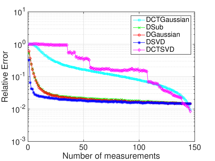
(a) San Francisco

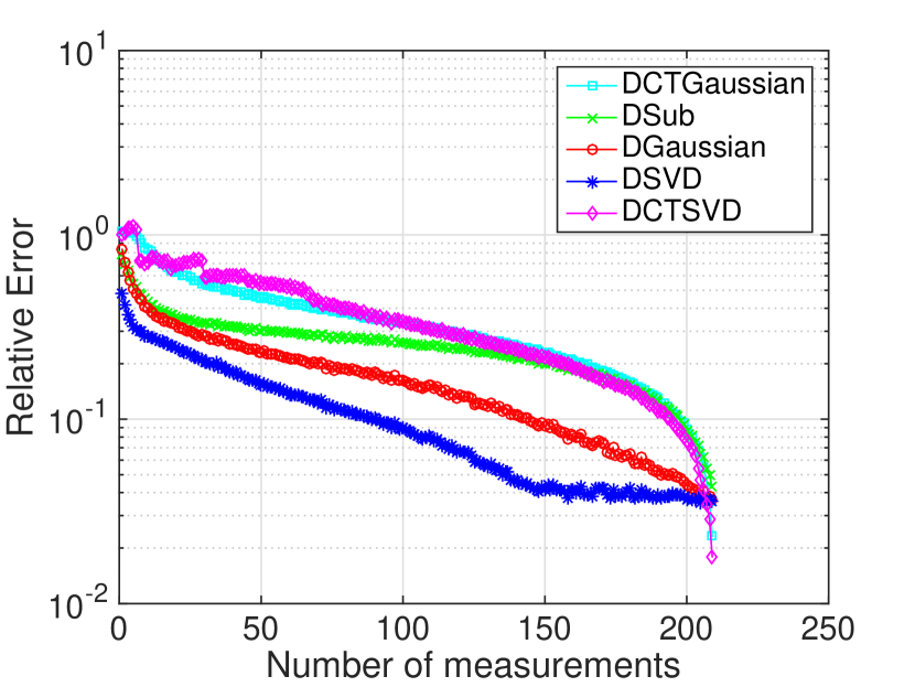
(b) Urban

Figure 2: Comparison among different sampling and sparsifying strategy combinations

For the case of 2-dimensional spatial images, it is well known that variants of the DCT and wavelet transforms provide effective sparsifying transformations. However, unlike the spatial domain, it turns out that neither the DCT nor wavelet transform provides sufficient compressibility in the spectral domain for effective CS reconstruction (see Figure 2 for example). We therefore turn our attention to learning a sparsifying dictionary that uses training or historical data of the scene of interest. In fact, it has been observed that learning a sparsifying dictionary from training datasets rather than using a predetermined sparsifying basis (e.g. DCT or wavelets) usually gives better sparse representation of the signal, and hence can improve the CS reconstruction results[27, 19]. Moreover, it has been discovered that the learned dictionary elements often represent the basic spectral signatures comprising the scene[9, 28]. Based on this, instead of using the random measurement matrices, we propose a new adaptive sampling strategy using the existing knowledge of the sparsifying dictionary of the spectral signals.

III-A Adaptive Sampling by SVD

One of the important factors for successful recovery using CS is the choice of the measurement matrix. It is now well known that many types of random matrices whose entries are drawn from Gaussian, Rademacher, or other sub-Gaussian distributions can act as the measurement matrices for any signal that is sparse with respect to an orthonormal basis. Researchers have also made substantial progress in the construction of sub-optimal deterministic universal measurement matrices to avoid the random effects[29, 30, 31]. Such measurement matrices are also used when the signal is sparse with respect to an overcomplete dictionary. However, all these constructions are for universal cases, which means they work for arbitrary $k$-sparse signals. Less attention has been paid to incorporating prior information, namely that a sparsifying dictionary may be obtained in advance for the application in hand. It is natural to ask the question whether we can sample smarter if the prior knowledge, such as a dictionary learned from training data, is available.

We here consider this problem by applying SVD to the sparsifying dictionary known in advance either from the analysis of historical data or learned by dictionary learning. Then the measurement matrix can be obtained by choosing the first $m$ singular vectors (associated with the first $m$ singular values in descending order) of the sparsifying dictionary. Specifically, the economical SVD of the sparsifying dictionary $D$ can be written as

$$D=U\Sigma V^{T},$$

where $U\in\mathbb{R}^{d\times d}$ contains the left singular vectors, $\Sigma\in\mathbb{R}^{d\times d}$ is a diagonal matrix containing all the singular vectors, and $V\in\mathbb{R}^{n\times d}$ contains the right singular vectors. Now let $U_{m}$ denote the submatrix of $U$ containing only the first $m$ columns of $U$. By setting the measurement matrix $\Phi=U_{m}^{T}$, we obtain a deterministic sampling strategy. Then the sampling process is simply a mixture of the signal of interest with fixed weights.

The reconstruction problem can be further simplified due to this special sampling strategy. Since

$$U_{m}^{T}D =U_{m}^{T}U\Sigma V^{T}$$

$$=\Sigma_{m}V_{m}^{T},$$

where $\Sigma_{m}$ is a diagonal matrix containing the $m$ largest singular values of the dictionary $D$ and $V_{m}$ contains the corresponding $m$ right singular vectors, we have from (3)

$$\min_{s}\|s\|_{1}\quad\text{such that}\quad\|y-\Sigma_{m}V_{m}^{T}s\|_{2}<\epsilon,$$ (8)

which can be solved using the SPGL1 solver.

III-B Matrix Balancing

A sufficient condition for CS to work is the Restricted Isometry Property (RIP)[32], which requires that the singular values of the sensing matrix do not vary too much. In other words, the sensing matrix needs to be well conditioned. We therefore further condition the sensing matrix by applying matrix balancing. Matrix balancing has been widely studied in various disciplines for square matrices [33, 34]. A square matrix is said to be balanced with respect to the $\alpha$-norm if for any index $i$, the $\alpha$-norm of the $i$th row is the same as that of the $i$th column. We here introduce a new balancing algorithm for general rectangular matrices based on SVD. We say an $m$ by $n$ ($m<n$) rectangular matrix is balanced if the row norms are the same as the column norms multiplied by a factor of $n/m$. The details of this algorithm is shown in Algorithm 1. It decomposes a given matrix $A$ into $A=PBQ$, where $P$ is a square invertible matrix, $Q$ is a nonsingular diagonal matrix, and $B$ is balanced in the sense that its rows are orthonormal and column norms only differ from the row norms by a constant factor provided the algorithm converges.

Algorithm 1 Matrix Balancing by SVD

1:  Input: matrix $A$, maximum number of iterations $t_{\max}$.

2:  Initialization: Set $t=1$, $B_{1}=A$, and $P_{1}$ and $Q_{1}$ to be identity matrices.

3:  while $t<t_{\max}$ do

4:     Perform SVD on $B_{t}$

$$B_{t}=U_{t}\Sigma_{t}V_{t}^{T}=U_{t}\Sigma_{t}(V_{t}^{T}S_{t})S_{t}^{-1},$$

where $S_{t}$ is a diagonal scaling matrix to normalize columns of $V_{t}^{T}$.

5:     Update:

$$P_{t+1}=P_{t}U_{t}\Sigma_{t},$$

$$B_{t+1}=V_{t}^{T}S_{t},$$

$$Q_{t+1}=S_{t}^{-1}Q_{t}.$$

6:  end while

7:  Output: matrix $A$ is decomposed into $A=P_{t_{\max}}B_{t_{\max}}Q_{t_{\max}}$, where $P_{t_{\max}}$ is nonsingular, $Q_{t_{\max}}$ is diagonal and nonsingular, $B_{t_{\max}}$ is balanced.

Now let $\tilde{y}=P^{-1}y$ and $\tilde{s}=Qs$. Then the minimization problem (1) can be rewritten as

$$\min_{\tilde{s}}\|Q^{-1}\tilde{s}\|_{0}\quad\text{subject to}\quad\tilde{y}=B\tilde{s}.$$ (9)

It is clear that $\tilde{s}$ has the same sparsity as $s$ since $Q$ is diagonal and nonsingular. Thus, problem (9) is equivalent to

$$\min_{\tilde{s}}\|\tilde{s}\|_{0}\quad\text{subject to}\quad\tilde{y}=B\tilde{s},$$

which is equivalent to the $\ell_{1}$ minimization problem

$$\min_{\tilde{s}}\|\tilde{s}\|_{1}\quad\text{subject to}\quad\tilde{y}=B\tilde{s}.$$

Similarly, it can also be written as a BPDN problem in presence of noise

$$\min_{\tilde{s}}\|\tilde{s}\|_{1}\quad\text{subject to}\quad\|\tilde{y}-B\tilde{s}\|_{2}<\epsilon.$$ (10)

Moreover, the sensing matrix is now better conditioned since it is normalized with respect to both rows and columns, and hence may improve the RIP constant since it is directly associated with the largest and smallest singular values of the submatrices. The BPDN problem (10) can be easily solved by using the SPGL1 solver.

In summary, our sampling and reconstruction procedure can be described as follows. We first find a sparsifying dictionary $D$ of the spectral signals of interest using dictionary learning based on training or historical data. We then construct a CS measurement matrix $U_{m}$ by applying SVD to the learned dictionary, using only the first $m$ significant singular vectors. Applying $U_{m}$ to the signal of interest yields a measurement vector of length $m$, which is less than the length of the signal of interest $n$. Now by feeding the measurement vector and the sensing matrix $A=U_{m}D$ into the standard CS solvers, we are able to obtain the signal of interest with length $n$.

IV Numerical Experiments

As discussed in Section III, the sparsifying transformations for 2-dimensional spatial images are well known. One can thus easily apply conventional CS methods in the spatial domain for efficient sampling. We now describe the results of numerical experiments that demonstrate the advantage of using the combination of dictionary learning and SVD over other combinations for the spectral domain signals.

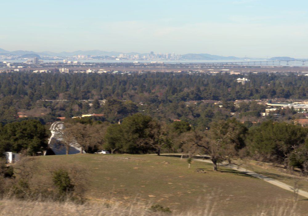
(a) San Francisco

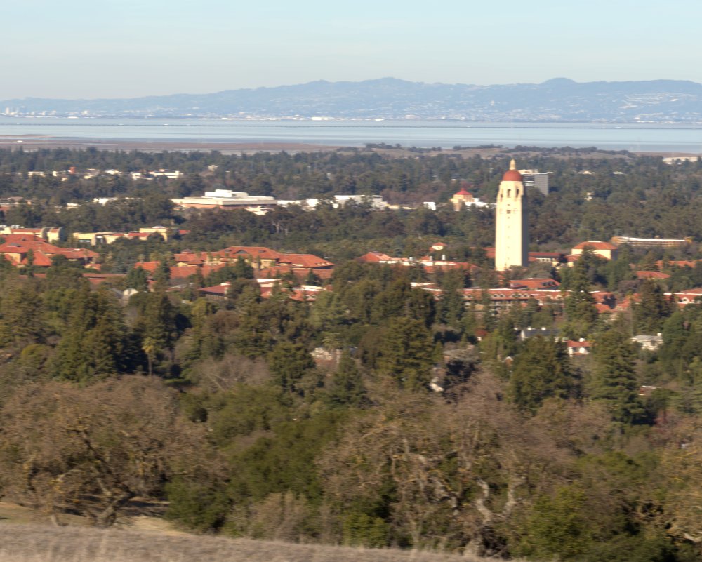
(b) Stanford Tower

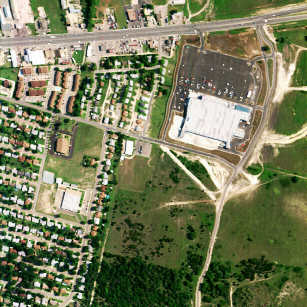
(c) Urban

Figure 1: RGB images of the three hyperspectral datasets used.

IV-A Dataset

In the following numerical experiments we will be using three hyperspectral datasets. The first two are both from the SCIEN lab at Stanford University [35]. The landscape hyperspectral image of San Francisco (SF) has a spatial resolution of 1000 $\times$ 702, and the hyperspectral image of the Stanford Tower has a spatial resolution of 1000 $\times$ 801, both containing 148 spectral bands ranging from 415nm to 950nm. The third dataset is the Urban dataset from the US Army Corps of Engineers, which is available at www.agc.army.mil/Missions/Hypercube.aspx. It has spatial resolution of 307 $\times$ 307, and contains 210 spectral bands ranging from 399nm to 2499nm.  Figure 1 provides a view of the three datasets as RGB images.

IV-B Comparisons of sampling and sparsifying strategies

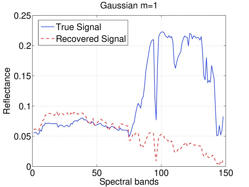
(a)

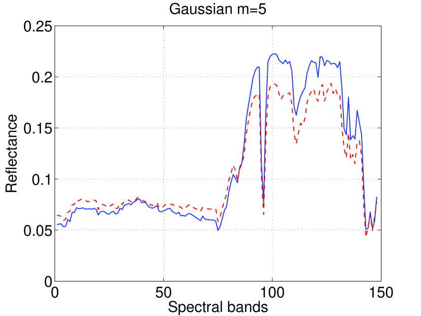
(b)

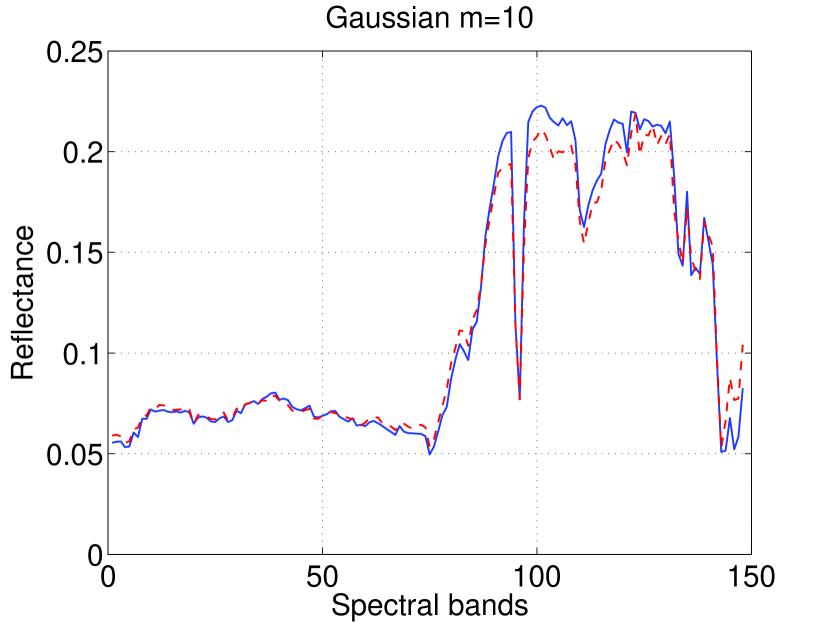
(c)

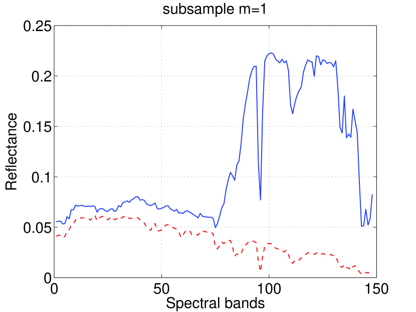
(d)

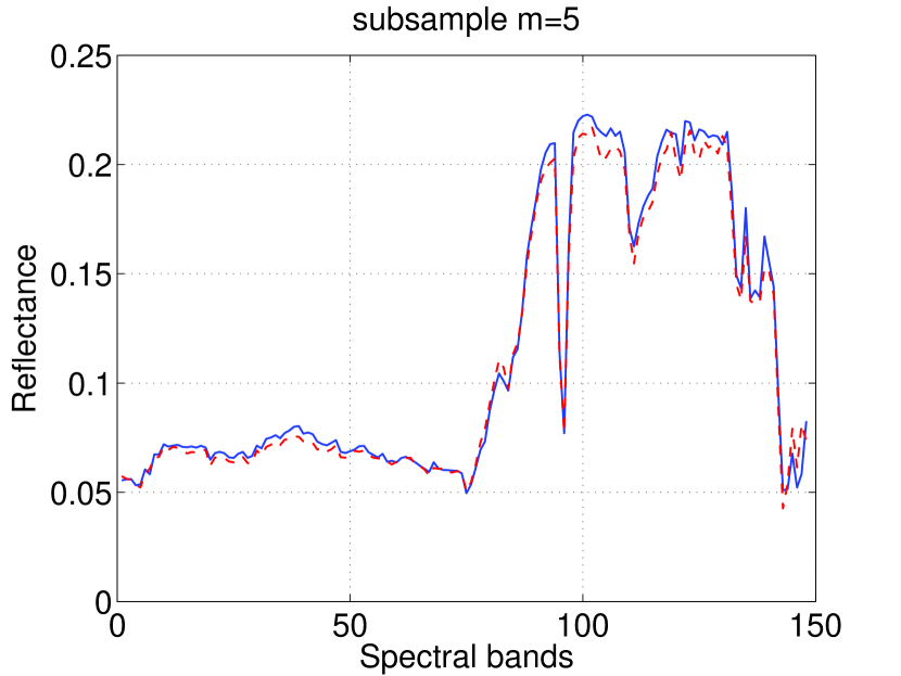
(e)

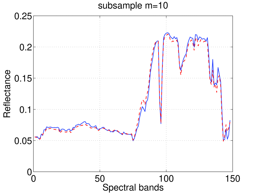
(f)

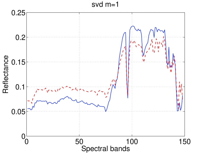
(g)

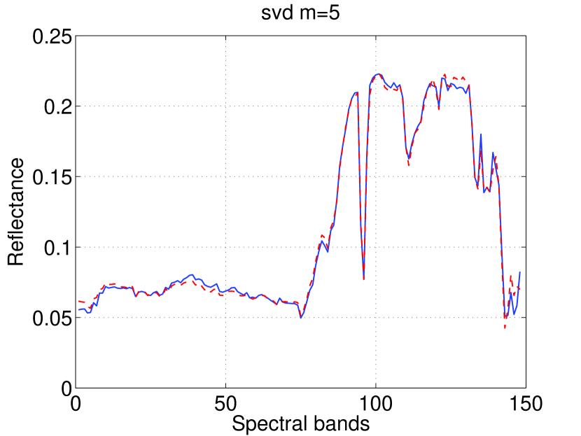
(h)

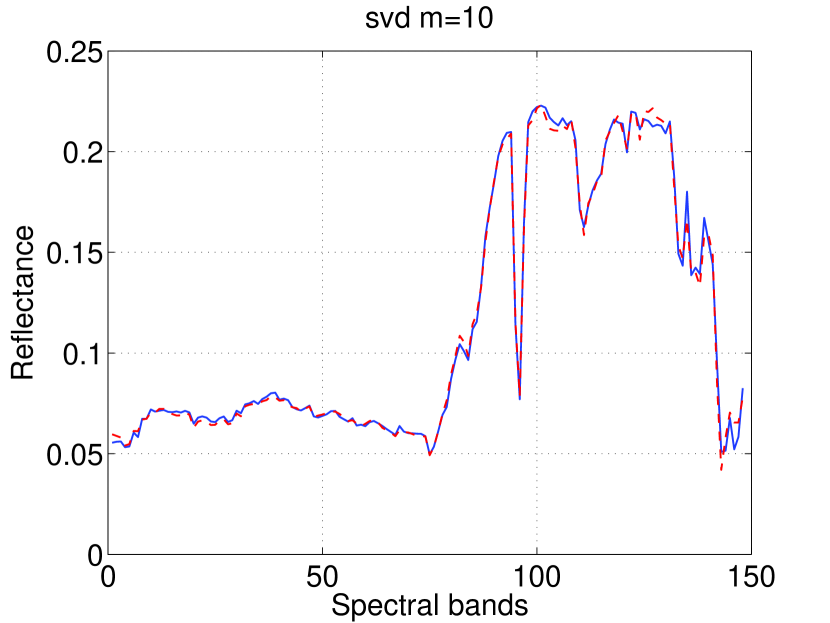
(i)

Figure 3: Comparison of the performance of different dictionary and measurement strategies combinations for a randomly chosen pixel in the San Francisco dataset. Figure (a)-(c) describe the reconstruction performance of DGaussian with different number of measurements $m$; figure (d)-(f) describe the reconstruction performance of DSub with different number of measurements $m$; figure (g)-(i) describe the reconstruction performance of DSVD with different number of measurements $m$.

The sparsifying dictionaries we use for our experiment are learned from the training data, which are obtained by randomly choosing half of the spectral signals (half of the pixels in the spatial domain) from the hyperspectral datasets mentioned above. The rest of the datasets are kept as the test data. We have normalized the hyperspectral data for each pixel to unit $\ell_{2}$ norm. We choose the error bound $\epsilon$ for BPDN in Eq. (3) to be $0.01$ and use the regularization parameter $\lambda=1.2/\sqrt{d}$ for sparse coding in Eq. (7), as suggested by [23]. Small variations of these parameters have yielded very similar performance. We now compare the performance of the five different combinations of sparsifying domains and sensing methodology using the SPGL1 solver. 2(a) and 2(b) compare their performance for the landscape hyperspectral image of San Francisco and the remote sensing hyperspectral image of an urban area respectively. Here DCTGaussian uses a DCT sparsifying matrix and a Gaussian measurement matrix. DSub means sparsifying matrix from dictionary learning and uniformly random subsampling. DGaussian stands for sparsifying matrix from dictionary learning with a Gaussian measurement matrix. DSVD stands for sparsifying matrix from dictionary learning with measurement matrix from SVD. We also include another combination DCTSVD, using DCT for the sparsifying matrix and SVD for the measurement matrix, for comparison. The relative error here is defined as

$$\text{Relative Error }=\frac{\|x^{*}-x\|_{2}}{\|x\|_{2}},$$

where $x^{*}$ is the reconstructed signal. It is clear from the plots that the conventional combination DCTGaussian does not provide efficient reconstruction, and performs much worse than the other combinations. In fact, it performs even worse than DSub, a naive choice of the measurement matrix combined with dictionary learning. The DCTSVD results are not good either as expected, since the DCT basis is a general sparsifying basis, which does not contain any information from the data. In addition, its singular values are all ones. Therefore, performing SVD on the DCT basis will not provide additional benefits. For the other three combinations, the combination DSub performs almost the same as DGaussian on the SF dataset, and worse on the Urban dataset as expected. The combination DSVD, as described in Section III, performs significantly better than the others on both datasets. One may notice that the performance for all the methods on the Urban data is worse than that on the SF data. This in fact coincides with our intuition. First of all, the number of measurements needed is directly related to the number of underlying spectral features mixed together in each pixel. In other words, it is related to how sparse the spectrum of the pixel is in terms of the learned dictionary. The SF data has a larger spatial resolution and relatively simpler spectral features, resulting in less mixtures for each pixel. While the Urban data has a smaller spatial resolution and much more complicated features, which could result in more feature mixtures in each pixel, and thus require larger number of measurements for good reconstruction.

We next give a more straightforward view of the reconstruction performance of the three combinations mentioned above using dictionary learning as the sparsifying domain, namely DSub, DGaussian, and DSVD. Figure 3 uses the same dataset as in 2(a), namely the SF dataset. All the figures describe the spectrum of the same randomly chosen pixel (representing woods in this case). We choose the number of measurements $m$ to be 1, 5, and 10 respectively. The blue curve is the ground truth of the spectrum for this pixel, while the red dashed curve is the reconstructed spectrum. As one can see, the Gaussian sampling and uniformly random subsampling strategies have about the same performance. They both fail when the number of measurement is 1 (0.68%) and start to recover the spectrum better with more measurements. The combination of dictionary learning with SVD performs the best in the sense that even when the number of measurement is 1, the reconstruction has already been able to catch a rough shape of the true spectrum and, when the number of measurement is 5 (3.38%), it can recover the true spectrum accurately.

The above results indicate that this approach can bring significant savings in cost, processing time, and storage. The amount of data generated by the conventional 2-D hyperspectral cameras causes difficulty for local storage or transmission. In contrast, with DSVD applied to the spectral domain, it is possible to store/transfer less than 5% of the original amount of data, which could be handled efficiently. For instance, the amount of data for a single $1000\times 1000\times 600$ hyperspectral cube to be stored/transmitted using conventional hyperspectral imager could easily reach 600 megabytes, while using the proposed strategy, it is less than 30 megabytes. Moreover, one may apply the conventional CS method, or even common image compression methods (e.g. JPEG) to the spatial images using the tensor structure as discussed in Section III to further improve the efficiency.

IV-C Matrix Balancing

Next we demonstrate that matrix balancing provides further enhancement in the reconstruction performance. The results of performing matrix balancing on the sensing matrix as described in Algorithm 1 for 10 iterations are shown in Figure 4.

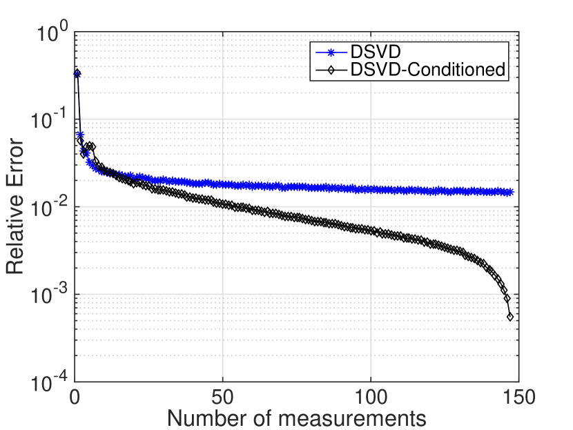
(a) San Francisco

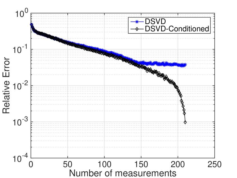
(b) Urban

Figure 4: Effect of sensing matrix balancing on reconstruction performance

From the figures we see clearly that matrix balancing does improve the reconstruction performance. However, the benefit is more significant on the SF dataset as shown in 4(a) than on the Urban dataset shown in 4(b).

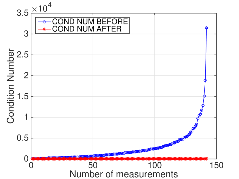
(a) San Francisco

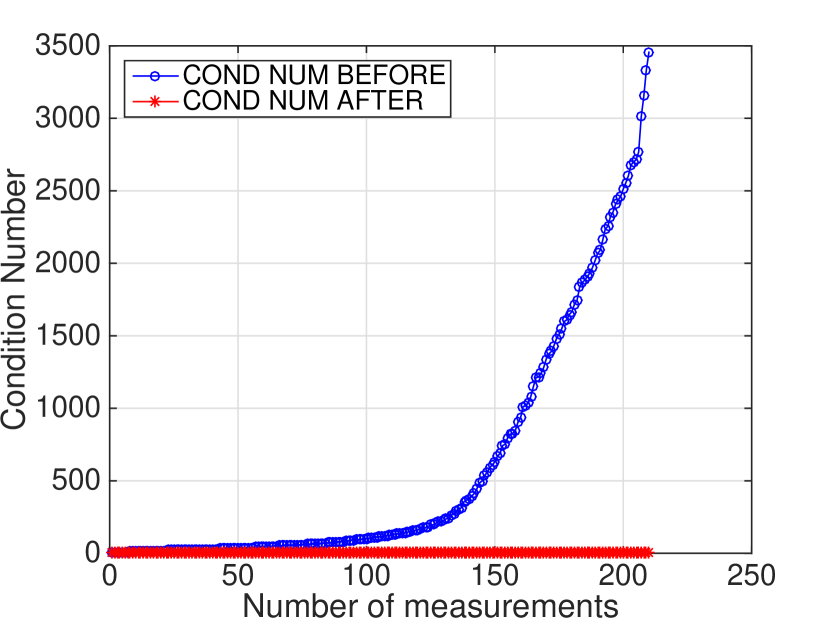
(b) Urban

Figure 5: Condition number of the sensing matrix before and after matrix balancing

To understand this phenomenon, we investigate the changes in condition numbers of the sensing matrices. Specifically, we check for both datasets the condition numbers of the sensing matrices with the number of measurements varying before and after performing matrix balancing. Figure 5 plots the behaviors of the condition numbers of the sensing matrices for both datasets. From the figures, the condition numbers for the sensing matrices for both datasets blow up as the number of measurements increases. Looking more closely though, the condition numbers of the sensing matrices for the SF dataset blow up significantly faster than that for the Urban data as the number of measurements approaches the full dimension, resulting in ill conditioned systems. Therefore, the reconstruction performance gain for the SF dataset is much better than that for the Urban dataset using matrix balancing as shown in Figure 4.

IV-D Robustness

The robustness of the dictionary learned from the training data has previously been studied in [9]. In that paper, authors learned the dictionary from the Smith Island training data and tested it on the test data collected on the same date. They showed by evaluation that the reconstruction relative MSE was less than 0.09% on that dataset. In addition, they also tested the dictionary learned on a test set collected in a different season for the same scene. They showed that the reconstruction relative MSE in this scenario was less than 0.71%, which was worse than for the test data collected on the same day but was still very good overall considering the vegetation and atmospheric characteristics were highly likely to be different due to different seasons.

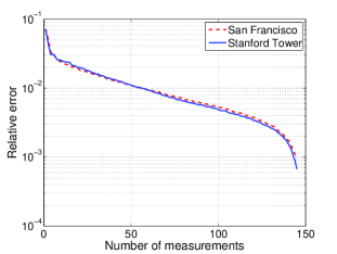
Figure 6: Robustness using San Francisco dictionary on Stanford Tower dataset.

Here we investigate, via numerical experiment, the robustness of the combination of dictionary learning and SVD on different datasets from different scenes. We first learn a dictionary from the San Francisco data and apply SVD to it to calculate a measurement matrix. This measurement matrix and dictionary is then used to compress and then reconstruct a different test data set, the Stanford Tower dataset. We then perform the same test on the Stanford Tower data, but this time using the dictionary and the corresponding measurement matrix learned from the data itself. Fig. 6 shows relative error curves of both approaches. As one can see, the relative error curve of reconstruction using the measurement matrix and the dictionary learned from the San Francisco data tested on the Stanford Tower data (dashed red curve) is very close to the result using the measurement matrix and the dictionary learned from the Stanford Tower data applied to itself (solid blue curve). In fact, the RMSE between these two error curves is less than 0.11%. This result indicates that our approach is robust even when applied to different, but similar scenes.

V Conclusion

In this paper, we proposed a new sampling strategy based on the existing knowledge of the sparsifying dictionary of the spectral signals we learned from the historical or training data to improve the sampling efficiency and the reconstruction performance for hyperspectral imaging. Specifically, a sparsifying dictionary was first learned from the training spectral data using dictionary learning. We then used the first $m$ left singular vectors as the fixed sampling pattern to obtain $m$ compressive measurements. Then the spectral signals were reconstructed using the SPGL1 solver based on the knowledge of the measurement matrix and the sparsifying dictionary. The reconstruction performance was further improved by reconditioning the sensing matrix using matrix balancing, especially when the sensing matrix became ill conditioned. It was also shown that our approach was robust to variations by applying the dictionary learned from the training data and its associated singular vectors to test data from different scenes.

References

- [1] J. Sanders, R. Williams, R. Driggers, and C. Halford, “A novel concept for hyperspectral remote sensing,” in Southeastcon ’92, Proceedings., IEEE, Apr 1992, pp. 363–367 vol.1.
- [2] T. Wilson and R. Felt, “Hyperspectral remote sensing technology (hrst) program,” in Aerospace Conference, 1998 IEEE, vol. 5, Mar 1998, pp. 193–200 vol.5.
- [3] E. Candes, J. Romberg, and T. Tao, “Robust uncertainty principles: exact signal reconstruction from highly incomplete frequency information,” Information Theory, IEEE Transactions on, vol. 52, no. 2, pp. 489–509, Feb 2006.
- [4] D. L. Donoho, “Compressed sensing,” IEEE Trans. Inform. Theory, vol. 52, no. 4, pp. 1289–1306, 2006. [Online]. Available: http://dx.doi.org/10.1109/TIT.2006.871582
- [5] M. Duarte, M. Davenport, D. Takhar, J. Laska, T. Sun, K. Kelly, and R. Baraniuk, “Single-pixel imaging via compressive sampling,” Signal Processing Magazine, IEEE, vol. 25, no. 2, pp. 83–91, March 2008.
- [6] Y. August, C. Vachman, Y. Rivenson, and A. Stern, “Compressive hyperspectral imaging by random separable projections in both the spatial and the spectral domains,” Appl. Opt., vol. 52, no. 10, pp. D46–D54, Apr 2013. [Online]. Available: http://ao.osa.org/abstract.cfm?URI=ao-52-10-D46
- [7] H. Zhang, J. Li, Y. Huang, and L. Zhang, “A nonlocal weighted joint sparse representation classification method for hyperspectral imagery,” Selected Topics in Applied Earth Observations and Remote Sensing, IEEE Journal of, vol. 7, no. 6, pp. 2056–2065, June 2014.
- [8] Y.-Q. Zhao and J. Yang, “Hyperspectral image denoising via sparse representation and low-rank constraint,” Geoscience and Remote Sensing, IEEE Transactions on, vol. 53, no. 1, pp. 296–308, Jan 2015.
- [9] A. Charles, B. Olshausen, and C. Rozell, “Learning sparse codes for hyperspectral imagery,” Selected Topics in Signal Processing, IEEE Journal of, vol. 5, no. 5, pp. 963–978, Sept 2011.
- [10] X. Lin, Y. Liu, J. Wu, and Q. Dai, “Spatial-spectral encoded compressive hyperspectral imaging,” ACM Trans. Graph., vol. 33, no. 6, pp. 233:1–233:11, Nov. 2014. [Online]. Available: http://doi.acm.org/10.1145/2661229.2661262
- [11] J. Hahn, S. Rosenkranz, and A. Zoubir, “Adaptive compressed classification for hyperspectral imagery,” in Acoustics, Speech and Signal Processing (ICASSP), 2014 IEEE International Conference on, May 2014, pp. 1020–1024.
- [12] R. Rana, M. Yang, T. Wark, C. T. Chou, and W. Hu, “Simpletrack: Adaptive trajectory compression with deterministic projection matrix for mobile sensor networks,” Sensors Journal, IEEE, vol. 15, no. 1, pp. 365–373, Jan 2015.
- [13] E. J. Candes, “The restricted isometry property and its implications for compressed sensing,” Comptes Rendus Mathematique, vol. 346, no. 9-10, pp. 589 – 592, 2008. [Online]. Available: http://www.sciencedirect.com/science/article/pii/S1631073X08000964
- [14] E. van den Berg and M. P. Friedlander, “SPGL1: A solver for large-scale sparse reconstruction,” June 2007, http://www.cs.ubc.ca/labs/scl/spgl1.
- [15] ——, “Probing the pareto frontier for basis pursuit solutions,” SIAM Journal on Scientific Computing, vol. 31, no. 2, pp. 890–912, 2008. [Online]. Available: http://link.aip.org/link/?SCE/31/890
- [16] H. G. Feichtinger and T. Strohmer, Eds., Gabor Analysis and Algorithms: Theory and Applications, 1st ed. Birkhauser Boston, 1997.
- [17] J.-L. Starck, M. Elad, and D. Donoho, “Redundant multiscale transforms and their application for morphological component separation,” in Advances in Imaging and Electron Physics, ser. Advances in Imaging and Electron Physics. Elsevier, 2004, vol. 132, pp. 287 – 348. [Online]. Available: http://www.sciencedirect.com/science/article/pii/S1076567004320069
- [18] J.-L. Starck, J. Fadili, and F. Murtagh, “The undecimated wavelet decomposition and its reconstruction,” Image Processing, IEEE Transactions on, vol. 16, no. 2, pp. 297–309, Feb 2007.
- [19] E. J. Candes, Y. C. Eldar, D. Needell, and P. Randall, “Compressed sensing with coherent and redundant dictionaries,” Applied and Computational Harmonic Analysis, vol. 31, no. 1, pp. 59 – 73, 2011. [Online]. Available: http://www.sciencedirect.com/science/article/pii/S1063520310001156
- [20] E. J. Candes and D. L. Donoho, “New tight frames of curvelets and optimal representations of objects with piecewise c2 singularities,” Communications on Pure and Applied Mathematics, vol. 57, no. 2, pp. 219–266, 2004. [Online]. Available: http://dx.doi.org/10.1002/cpa.10116
- [21] H. Lee, A. Battle, R. Raina, and A. Y. Ng, “Efficient sparse coding algorithms,” in Advances in Neural Information Processing Systems 19, 2007, pp. 801–808.
- [22] O. Bousquet and L. Bottou, “The tradeoffs of large scale learning,” in Advances in Neural Information Processing Systems 20, J. Platt, D. Koller, Y. Singer, and S. Roweis, Eds. Curran Associates, Inc., 2008, pp. 161–168. [Online]. Available: http://papers.nips.cc/paper/3323-the-tradeoffs-of-large-scale-learning.pdf
- [23] J. Mairal, F. Bach, J. Ponce, and G. Sapiro, “Online dictionary learning for sparse coding,” in Proceedings of the 26th Annual International Conference on Machine Learning, ser. ICML ’09. New York, NY, USA: ACM, 2009, pp. 689–696. [Online]. Available: http://doi.acm.org/10.1145/1553374.1553463
- [24] B. Efron, T. Hastie, I. Johnstone, and R. Tibshirani, “Least angle regression,” Ann. Statist, p. 2004.
- [25] M. Osborne, B. Presnell, and B. Turlach, “A new approach to variable selection in least squares problems,” IMA Journal of Numerical Analysis, vol. 20, no. 3, pp. 389–403, 2000. [Online]. Available: http://imajna.oxfordjournals.org/content/20/3/389.abstract
- [26] D. P. Bertsekas, Nonlinear Programming, 2nd ed. Athena Scientific, Sep. 1999. [Online]. Available: http://www.amazon.com/exec/obidos/redirect?tag=citeulike07-20&path=ASIN/1886529000
- [27] M. Aharon, M. Elad, and A. Bruckstein, “k -svd: An algorithm for designing overcomplete dictionaries for sparse representation,” Signal Processing, IEEE Transactions on, vol. 54, no. 11, pp. 4311–4322, Nov 2006.
- [28] J. Greer, “Sparse demixing of hyperspectral images,” Image Processing, IEEE Transactions on, vol. 21, no. 1, pp. 219–228, Jan 2012.
- [29] R. A. DeVore, “Deterministic constructions of compressed sensing matrices,” Journal of Complexity, vol. 23, no. 4–6, pp. 918 – 925, 2007, festschrift for the 60th Birthday of Henryk Woźniakowski. [Online]. Available: http://www.sciencedirect.com/science/article/pii/S0885064X07000623
- [30] S. Jafarpour, W. Xu, B. Hassibi, and R. Calderbank, “Efficient and robust compressed sensing using optimized expander graphs,” Information Theory, IEEE Transactions on, vol. 55, no. 9, pp. 4299–4308, Sept 2009.
- [31] J. Bourgain, S. Dilworth, K. Ford, S. Konyagin, and D. Kutzarova, “Explicit constructions of rip matrices and related problems,” Duke Math. J., vol. 159, no. 1, pp. 145–185, 07 2011. [Online]. Available: http://dx.doi.org/10.1215/00127094-1384809
- [32] E. Candes and T. Tao, “Decoding by linear programming,” Information Theory, IEEE Transactions on, vol. 51, no. 12, pp. 4203–4215, Dec 2005.
- [33] T.-Y. Chen and J. W. Demmel, “Balancing sparse matrices for computing eigenvalues,” Linear Algebra and its Applications, vol. 309, no. 1–3, pp. 261 – 287, 2000. [Online]. Available: http://www.sciencedirect.com/science/article/pii/S0024379500000148
- [34] P. A. Knight and D. Ruiz, “A fast algorithm for matrix balancing,” IMA Journal of Numerical Analysis, 2012. [Online]. Available: http://imajna.oxfordjournals.org/content/early/2012/10/26/imanum.drs019.abstract
- [35] T. Skauli and J. Farrell, “A collection of hyperspectral images for imaging systems research,” pp. 86 600C–86 600C–7, 2013. [Online]. Available: http://dx.doi.org/10.1117/12.2007097