Octupole Focusing Relativistic Self-Magnetometer Electric Storage Ring “Bottle”

Abstract

A method proposed for measuring the electric dipole moment (EDM) of a charged fundamental particle such as the proton, is to measure the spin precession caused by a radial electric bend field $E_{r}$, acting on the EDMs of frozen spin polarized protons circulating in an all-electric storage ring. The dominant systematic error limiting such a measurement comes from spurious spin precession caused by unintentional and unknown average radial magnetic field $B_{r}$ acting on the (vastly larger) magnetic dipole moments (MDM) of the protons. Along with taking extreme magnetic shielding measures, the best protection against this systematic error is to use the storage ring itself, as a “self-magnetometer”; the exact magnetic field average $\langle B_{r}\rangle$ that produces systematic EDM error, is nulled to exquisite precision by orbit position control.

The self-magnetometry sensitivity depends inversely on the restoring force with which the storage ring opposes the magnetic field $\langle B_{r}\rangle$. By using octupole rather than quadrupole focusing (which the name “bottle”, copied from low energy physics, is intended to convey) the restoring force can be vanishingly small for small amplitude vertical betatron-like motion while, at the same time, being strong enough at large amplitudes to keep all particles captured. This greatly enhances the magnetometer sensitivity.

In a purely electric ring clockwise (CW) and counter-clockwise (CCW) orbits would be identical, irrespective of ring positioning and powering errors. In the absence of magnetic fields this symmetry is guaranteed by time reversal invariance (T). However, any average radial magnetic field error $\langle\Delta B_{r}\rangle$ causes a vertical orbit shift between CW and CCW beams.

Self-magnetometry measures this shift, enabling its cancellation. For the octupole-only ring proposed here the accuracy of magnetic field control is $\langle\Delta B_{r}\rangle\approx\pm 3\times 10^{-16}\,$Tesla. This is small enough to reduce the systematic error in the proton EDM measurement into a range where realistically small deviations from standard model predictions can be measured.

Though novel, the theoretical analysis given here for relativistic bottles, either magnetic or electric, is elementary, and their behavior is predicted to be entirely satisfactory. For particles other than p and e, combined magnetic plus electic rings are needed, but the same sefl-magnetometry should be applicable.

I Introduction

For a fundamental particle such as the proton to have a non-zero electric dipole moment (EDM) would violate both time reversal (T) and parity (P) symmetries. Both of these symmetries are, in fact, violated in the standard model, but too weakly to account for the observed matter-antimatter imbalance in the universe. This motivates measuring the proton EDM. This will require trapping an intense polarized proton beam in a “frozen spin” all-electric storage ring “trap”. Even in an electric field the spin precession of a moving proton is dominated by the motional magnetic field in the proton’s rest frame, acting on the magnetic dipole moment (MDM). But, the EDM and MDM precessions can be distinguished, because their precession axes are orthogonal.

An ideal configuration for precision measurement of elementary particle parameters, such as magnetic dipole moments, would maintain the particles in a wall-free configuration stabilized by the electrostatic interaction of the charges. Earnshaw’s theorem proves this to be impossible. Nevertheless, by introducing RF cavities, lasers, etc., not covered by the theorem, it has been possible to store low energy particles indefinitely in various “bottles” or “traps”. Relativistic charged particles can even be stored, wall-free, in storage rings, which rely on quadrupoles, solenoids, field gradients, or pole-edge rotation, to provide the “linear” focusing traditionally thought to be necessary to keep the particles captured.

This paper proposes an electric “bottle” capable of storing an intense beam of relativistic protons (or electrons, or other charged particles). Except for RF cavity (required to provide longitudinal, bunched beam, stability) and occasional brief “reflections” from octupole fields, the particles survive indefinitely, most of the time in nearly uniform fields. This proposal has been motivated primarily by the requirements for measuring the proton electric dipole moment (EDM) or, more particularly, by the need to suppress the most important systematic error limiting that measurement. The reflection mechanism resembles the end reflections in (non-relativistic) “magnetic mirror machines” developed independently by Post in the U.S.A. and Budker in the U.S.S.R. But, unlike those devices, small amplitude particles cannot escape the proposed trap.

Various designs have been proposed for measuring the electric dipole moments of charged particles, especially the protonFreqDomainEDM BNLproposal and electron, in all-electric, frozen spin, storage rings. For an all-electric ring any non-zero EDM will cause spin precession about an axis forbidden by P and T symmetry. The overwhelmingly most serious background will be due to the presence of radial magnetic field $\Delta B_{r}$. Here the $\Delta$ connotes that the field would ideally be zero, and the $r$ is the radially outward coordinate. (Following standard accelerator terminology, the $E_{r}$ field will, where appropriate, be expressed as $E_{x}$, where $x$ is the radial component in a local, Frenet coordinate system.) The field $\Delta B_{x}$, acting on the particle magnetic moment, causes precession that exactly mimicks the precession caused by the primary bending electric field, $E_{x}$, acting on the (vastly weaker) EDM. Even with $\Delta B_{x}$ reduced to the extent possible, it will be challenging to reduce the systematic error to a value small enough to provide a serious test of the standard model (which predicts a value $d_{p}$ less than $10^{-30}\,$e-cm, for the proton EDM).

Reducing $\Delta B_{x}$ is not the only motivation for all-electric bending. Electric bending also permits reversing the beam direction of circulation without changing any ring parameters. With vanishing magnetic fields, time reversal invariance, guarantees that all particle orbits are exactly preserved (except in direction) when the injection direction is reversed, irrespective of positioning and powering errors. Any magnetic field error $\Delta B_{x}$ will move all the beam orbits up or down, depending on the average $\langle\Delta B_{x}\rangle$. Reversing the beam direction will reverse this shift. The most effective way of reducing the magnetic field error will be to use the ring as a “self-magnetometer”, with the vertical beam position measured by beam position monitors (BPMs), to adjust magnetic vertical steering elements to eliminate the average vertical orbit shift when the beam direction is reversed.

Vertical focusing limits the effectiveness of this approach. With no vertical focusing one could dream that, if the clockwise (CW) beam is lost in the up-direction then the CCW beam would be lost in the down-direction. In fact, because of vertical focusing, no beam at all is, in fact, lost. The best one can do is to design the ring to maximize the measurable vertical orbit shift when the beam direction is reversed. Nonlinear (octupole) focusing can be strong enough at large amplitudes to avoid particle loss, yet weak enough at small amplitudes to permit precise magnetometry.

The approach to be taken can be motivated by an analogy. The weight of a fish can be determined by hanging the fish from a spring whose length is measured by a linear scale. To serve for both small and big fish, with scale of convenient length, the spring constant would be strong. For better accuracy for small fish, the spring constant would be weak. The ideal spring would be weak for small fish but strong for big fish. An octupole has just this character: its field gradient is negligible for small displacements, strong for large displacements.

But accelerator focusing behavior is more complicated. Quadrupoles in accelerator lattices, if focusing in one plane, say vertical, are defocusing in the other plane. Something like this also applies to octupole focusing, though, for small amplitudes, a vertically focusing octupole is also horizontally focusing. But we need only very weak vertical focusing. We therefore anticipate a region of phase space near the origin for which the vertical focusing is weak. Meanwhile the relatively strong horizontal geometric focusing is much stronger than the octupole focusing.

II Orbit Equations for the Storage Ring Bottle

The simplest possible electrostatic ring consists of coaxial cylindrical electrodes, of inner and outer radii $r_{0}\mp g/2$, where $g$ is the gap width between the electrodes. A sector of such a ring is shown in Figure 1.

Figure 1: The bold curve shows a proton orbit passing through a curved-planar cylindrical electrostatic bending element. The electrode spacing is $g$ and the design orbit is centered between the electrodes. The electric lattice in this paper has 281 m circumference, consisting of 16 indentical bends like this, each with arc length 15.7 m arc length, with the remainder of the circumference taken up by straight sections.

In a cylindrically-symmetric electrostatic potential $\phi(r,z)$, producing a predominantly-radial electric field $-E{\bf\hat{r}}$, beam particles of charge $e$ move in approximately circular orbits close to a horizontal $(x,z)$ plane. The $y$ coordinate is normal to the plane. On the circular design orbit the centripetal electric force is provided by the radial electric field $E_{r}$;

$$\frac{p_{0}v_{0}}{r_{0}}=-eE_{r}$$ (1)

With $s$ being a global longitudinal arc length parameter, and local Frenet coordinates $(x,y,z)$, which are incremental offsets, radial, vertical, and longitudinal (i.e. tangential to the design orbit), the betatron equations areETEAPOT1

$$\frac{d^{2}x}{ds^{2}} =-\bigg{(}\frac{1}{r^{2}_{0}}+\frac{1}{\gamma_{0}^{2}r^{2}_{0}}\bigg{)}\,x=-\frac{1.64}{r^{2}_{0}}\,x,$$ (2)

$$\frac{d^{2}y}{ds^{2}} =0.$$ (3)

Here the numerical value 1.64 has come from choosing $\gamma_{0}$ appropriate for frozen spin proton operation (for which this paper is primarily intended). The relativistic factor $\gamma_{0}=\mathcal{E}/m_{p}c^{2}=1/\sqrt{1-v_{p}^{2}/c^{2}}$ has the “magic” value $\gamma_{0}=1.25$ at which the proton spins are “frozen” (for example, always parallel to the orbit.) This corresponds to proton kinetic energy $K_{p}=0.233\,$GeV, velocity $\beta_{p}c=0.60c$, and momentum $p_{p}c=0.70\,$GeV—relativistic, but not very relativistic.

Eqs. (2) and (3) differ only slightly from the equations for a traditional weak focusing magnetic ring. The second shows there is no vertical focusing, meaning the beam will eventually be lost vertically. Vertical stability can be easily restored by contouring the poles slightly (combined function) or introducing vertically focusing quadrupoles (separated function). Both of these constitute “linear focusing” which, according to ground rules of the present paper, is not to be allowed (in the interest of maximal magnetometry sensitivity.) One can object that the term $\big{(}x/r^{2}_{0}+x/(\gamma_{0}^{2}r^{2}_{0})\big{)}$ in the $x$ equation also constitutes “linear focusing”. But this is “geometric” focusing which (by a convention adopted just for this paper) is allowable (in fact, essential). The same terminology is standard for a cyclotron—it is geometric focusing that permits the deviation from the design circular orbit to a slightly deviant circular orbit to be described as a horizontal betatron oscillation crossing the design orbit twice per revolution, as if due to focusing. The extra term $x/(\gamma_{0}^{2}r^{2}_{0})$ in the horizontal focusing is specific to electrostatic focusing.

Unlike in a magnetic field, in an electric field the particle velocity is not conserved, causing the $\gamma$ factor to deviate from $\gamma_{0}$ as the electric potential deviates from zero. But to a first (good) approximation, the orbits are described by Eqs. (2) and (3). The only significant effect of the ring being electrostatic is that the extra term $x/(\gamma_{0}^{2}r^{2}_{0})$ makes the horizontal focusing somewhat stronger than in an old-fashioned, weak-focusing magnetic ring.

Neglecting the perturbing effects of the short straight sections between bend elements, in terms of a “betatron phase” $\psi_{x}(s)$ which, for this simple ring, is proportional to $s$, and beta function $\beta_{x}(s)$, which is actually independent of $s$, in pseudo-harmonic form, the cosine-like $x$ motion for a particle with betatron amplitude $a_{x}$ is

$$x(s)=a_{x}\sqrt{\beta_{x}(s)}\cos\big{(}\psi_{x}(s)\big{)}=a_{x}\sqrt{\beta_{x}}\cos\frac{s}{\beta_{x}},$$ (4)

where

$$\psi_{x}(s)=\int_{0}^{s}\frac{ds^{\prime}}{\beta_{x}(s^{\prime})}=\frac{s}{\beta_{x}},$$ (5)

Because $\beta_{x}(s)$ is independent of $s$ the integral is trivial. In summary:

$$x(s) =A_{x}\cos\bigg{(}\sqrt{\frac{1+1/\gamma_{0}^{2}}{r^{2}_{0}}}\,s\bigg{)},$$

$$y(s) =A_{y}+{\rm constant}\,\times s.$$ (6)

Matching $x$ arguments gives

$$\beta_{x}=\frac{r_{0}}{\sqrt{1+1/\gamma_{0}^{2}}},\quad\Big{(}\overset{\rm e.g.}{\ =\ }0.78\times 40=31\,{\rm m}\Big{)}.$$ (7)

The phase advance per turn $\mu_{x}$ and the tune $Q_{x}=\mu_{x}/(2\pi)$ are obtained by matching $x$ arguments to give

$$Q_{x}=\frac{r_{0}}{\beta_{x}}=\sqrt{1+\frac{1}{\gamma_{0}^{2}}}\quad\Big{(}\overset{\rm pEDM}{\ =\ }1.281\Big{)},$$ (8)

and $Q_{y}=0$.

II.1 Distributed Octupole Field

One way or another, the vertical motion has to be stabilized. To do this we introduce an octupole field, assumed to be uniformly distributed around the ring, with local octupole moment per unit length $o=O/(2\pi r_{0})$. (For numerical simulations shown later in this paper the “uniform octupole distribution” is modeled as 16 lumped octupoles, one in each straight section.) The orbit equations become

$$\frac{d^{2}x}{ds^{2}} =-\frac{1.64}{r^{2}_{0}}\,x-\frac{o}{6}\,(x^{3}-3xy^{2})-qx+f_{x},$$ (9)

$$\frac{d^{2}y}{ds^{2}} =\frac{o}{6}\,(3x^{2}y-y^{3})+qy+f_{y}.$$ (10)

As well as the octupole termsUSPASmanual , for later convenience, we have included other small terms that can be neglected initially. A possible distributed “trim” quadrupole is represented by the terms $-qx$ and $+qy$; positive $q$-value introduces (very weak) horizontal focusing and vertical defocusing. Also added are constant “force” terms $f_{x}$ and $f_{y}$.

This paper concentrates on the added term $f_{y}$ which represents an unknown magnetic “force” that needs to be cancelled. The term $f_{x}$ will eventually be set to zero based on the following comments. Though $x$ and $y$ are locally orthogonal, only $y$ is fixed globally, while $x$ is a Frenet coordinate, always radial. A constant radial force is best treated as a change in radius of curvature, leaving the orbit plane invariant, but changing the design orbit radius. A constant vertical force, on the other hand, tends to make an otherwise-planar orbit helical, leading to a gradual vertical displacement of the whole orbit.

The octupole terms, as well as being nonlinear, also couple the $x$ and $y$ motion. Solving these equations analytically and in general for all amplitudes is clearly impossible, even if for no other reason than that the motion will become chaotic for sufficiently large amplitudes. If the equations are to describe anything practical, they will have to apply only to appropriately small amplitudes. Fortunately this will be applicable for electrostatic rings appropriate for measuring EDMs. To obtain large electic field $E_{y}$ it is important for electrode gap $g$ to be small. This forces the horizontal ring acceptance to be small. On the other hand it is feasible for the vertical acceptance to be almost arbitrarily large. Unbalanced acceptance like this is favorable for octupole focusing.

II.2 Guiding Center Approximation

We are interested primarily in two effects influencing the vertical orbit motion. One is the role played by the electrostatic octupole field present for limiting the vertical motion. Each particle gyrates rapidly while advancing slowly in the vertical direction, oscillating up and down as the octupole field occasionally causes it to reflect, down from the top or up from the bottom. The other effect to be included is the systematic vertical orbit shift caused by any residual constant radial magnetic field. Sensitivity to this shift, opposite for CW and CCW orbit circulation direction, is the basis of the self-magnetometry function.

Language here has been chosen to suggest the non-relativistic orbit of a particle gyrating around a field line in a slowly varying magnetic field, for example in a magnetic bottle or in the earth’s ionosphere. With each orbit gyrating rapidly around a “guiding center”, it is adequate to describe the motion of the guiding center, rather than following the charged particle itself. In our relativistic storage ring with ultraweak vertical focusing, each particle moves in a helical orbit, always in an almost closed circle of radius $r_{0}$, perhaps 40 m. The guiding center hardly moves from the center of the ring, mainly just up and down by, at most, a few centimeters.

The guiding center formalism is appropriate for describing a storage ring relativistic bottle with uniform vertical magnetic field. This theory is sketched concisely in the Section VII appendix. To corroborate applying this theory to magnetic storage rings some TEAPOTTEAPOT UAL simulations of a magnetic storage ring bottle are shown later in this paper. But we are primarily interested in an the electric storage ring bottle, to be modeled later using ETEAPOTETEAPOT1 . First the equations are solved approximately.

II.3 Fast-Slow Approximation

Ordinarily, in storage rings, a fast-slow approximation is used in which synchrotron (energy) oscillations are “slow” enough to be treated as “adiabatic” (i.e. essentially constant) as regards their influence on $x$ and $y$ betatron oscillations. Slightly different approximations are appropriate in the present situation. Only $x$ oscillations are fast; longitudinal $z$ and vertical $y$ oscillations are slow.

Part of the justification for this picture is based on the particular configuration being discussed, which can be refreshed by reviewing Figure 1. Because practical electric forces are vastly weaker than magnetic forces, to produce sufficiently large electric field the electrode gap $g$ is necessarily small, 2 or 3 cm. This restricts the horizontal amplitude $a_{x}\sqrt{\beta_{x}}$ to be quite small. On the other hand, for any stable vertical oscillations, the absence of linear focusing will certainly cause the vertical tune $Q_{y}$ to be very small. Furthermore, since the electrodes can be almost arbitrarily high, the vertical coordinate $y$ is allowed to be quite large, much larger than $x$.

This suggests approximating $x^{2}$ by its average value while treating the $y$ motion. In Eq. (10) we set $x^{2}=\sigma_{x}^{2}$, where $\sigma_{x}\approx g/4$ is an approximate r.m.s. value of $x$ for a parabolic-shaped proton beam in a chamber with width $g$. The result is

$$\frac{d^{2}y}{ds^{2}}=\bigg{(}\frac{og^{2}}{32}+q\bigg{)}\,y+\frac{o}{6}\,y^{3}+f_{y}.$$ (11)

(The “trim quadrupole” term $+qy$ reserves the possibility of empirically cancelling the $y$-term, at least approximately, by tuning the value of the parenthesized term to zero.)

Though now decoupled, this equation is still nonlinear. However, since the right hand side is a function only of $y$, the orbit description can be simplified by introducing (conserved) “energy” $h$,

$$h=\frac{1}{2}\,\bigg{(}\frac{dy}{ds}\bigg{)}^{2}-\bigg{(}\frac{og^{2}}{64}+\frac{q}{2}\bigg{)}\,y^{2}-\frac{o}{24}\,y^{4}-f_{y}y.$$ (12)

(The energy symbol “h” introduced here has been chosen the same as an analogous symbol for energy, in the Section VII appendix for mnemonic convenience. Though the “h” roles are analogous in the two contexts, their physical dimensions differ for inessential reasons of convenience. A dimensional factor needed to restore dimensional consistency and a relativistic correction, not very important for $\gamma=1.25$ protons, will be introduced later.) Much of the vertical motion can then be inferred from curves of constant $h$ in $(y,dy/ds)$ phase space. Numerical solutions, using MAPLE, are shown in Figure 2. As well as exhibiting three amplitudes, the figure also allows for the presence of a small $f_{y}$ term, of either sign, black for positive, green for negative. The “vertical force sensitivity” is the beam centroid deviation divided by the vertical “force” which, in this case is $0.06/0.00001=0.6\times 10^{4}$ (in the units implied by the numerical form given at the top of the figure).

The corresponding $x$-equation, with $y=y_{c}$ (with $y_{c}$ treated as varying adiabatically, and hence effectively constant, with value $0$) is

$$\frac{d^{2}x}{ds^{2}} =-\bigg{(}\frac{1.64}{r^{2}_{0}}+\frac{o}{6}\,y_{c}+q\bigg{)}\,x-\frac{o}{6}\,x^{3}+f_{x}.$$ (13)

Numerical determinations of the phase trajectories are shown in Figure 3.

Comparing Figures 2 and 3, one sees that the vertical sensitivity to $f_{y}$ is two orders of magnitude greater than the horizontal sensitivity to $f_{x}$. Of course this is because the horizontal focusing is of linear order, while the vertical focusing is of octupole order. In “typical” storage rings the horizontal and vertical focusing strengths are comparable, which is manifested by their radial and vertical tunes $Q_{x}$ and $Q_{y}$ being comparable in magnitude. Our storage ring bottle lattice has therefore achieved the goal of increasing the vertical force sensitivity by a factor of about 100, compared to typical rings.

This comparison is somewhat misleading howerer, for reasons alluded to earlier. The main effect of reversing $f_{x}$ suddenly is a change in gross orbit radius. But there is also the net radial orbit shift shown in Figure 3. The global direction of this shift would depend on the particle azimuthal position when the force was reversed. As such the shift is not directly commensurate with the vertical magnetometer orbit shift which is the subject of this paper. Also this comparison does not take advantage of potentially increased magnetometer sensitivity using quadrupole $q$ to tune the linear focusing coefficient more nearly to zero.

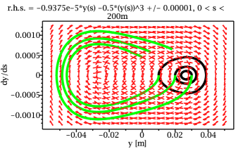
Figure 2: Vertical phase space trajectory dependence on constant vertical force in storage ring bottle with radial geometric focusing plus octupole (but no quadrupole) focusing. Curves with +/- constant force are black/green. “r.h.s.” stands for the right hand side of Eq. (11). The magnetometer sensitivity is proportional to the displacement of black relative to green. The plot was obtained using MAPLE.

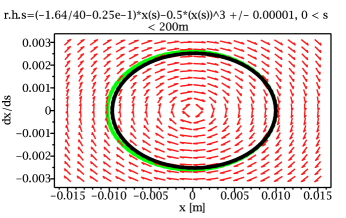
Figure 3: Sensitivity of horizontal phase space trajectory to constant horizontal force in storage ring bottle with radial “geometric” focusing plus octupole focusing. “r.h.s.” stands for the right hand side of Eq. (13). Curves with +/- constant force are black/green. The magnetometer sensitivity is proportional to the displacement of black relative to green. The plot was obtained using MAPLE.

II.4 Octupole Restrained Motion

Relativistic orbits in a magnetic bottle are analysed in the appendix, following formalism standard in plasma physics. However, the adiabatic invariance of the product of effective current $\times$ enclosed area, which is central to the magnetic bottle treatment, may not be valid for an electric bottle, especially because the electric potential depends on position. Nevertheless, since the orbits have already been seen to be so similar, one expects reflections down from the top and up from the bottom to be subject to similar analyses.

When it passes through the $y=0$ horizontal design plane, a given particle has vertical momentum $p_{y0}$ which is, let us say, positive, and certainly very small compared to its total momentum $p_{0}$. Because $p_{y0}<<p_{0}$, the helical orbit is scarcely distinguishable from a perfect circle. For many turns, because the octupole is so weak near the origin, $p_{y}$ remains essentially constant. But, eventually, the integrated effect of the octupole field is sufficient to reflect the vertical motion. The magnitude $y_{\rm t.p.}(p_{y0})$ of the vertical turning point of the $y$-motion clearly increases with increasing $|p_{y0}|$.

Comparing Eq. (12) with Eq. (38) in the Section VII appendix, one sees that vertical motion (perpendicular to electric field) in an electric bottle, is subject to much the same analysis as longitudinal motion (parallel to magnetic field lines) in a magnetic bottle. In each case the particle moves more or less freely parallel to the axis of the bottle, but is occasionally restrained by reflection from turning points at one or the other end of the bottle. In the electric bottle the “vertical energy” of a particle with slope $y^{\prime}_{0}$ at the center of the bottle is $h_{0}=\gamma_{0}{y_{0}^{\prime}}^{2}/2$; use of the non-relativistic energy formula (slightly modified by the $\gamma_{0}$ factor accounting for inertial mass) will be justified shortly. At the turning points, at the bottle ends, $y^{\prime}=0$. Substituting into Eq. (12), with $q=0$ and $f_{y}=0$ produces

$$y_{tp}^{4}+\frac{3}{8}\,g^{2}y_{tp}^{2}+\frac{12}{o}\,\gamma_{0}{y_{0}^{\prime}}^{2}=0.$$ (14)

(For magic energy protons the relativistic correction is small, and is being neglected in this paper. But, for magic energy electrons the relativistic factor is $\gamma_{0}=30$, giving a significant relativistic correction even if the vertical component of velocity is non-relativistic.) Solving for $y_{tp}$ produces

$$y_{tp}=\frac{\pm 1}{\sqrt{2}}\,\sqrt{-\frac{3}{8}\,g^{2}+\sqrt{\frac{9}{64}\,g^{4}-\frac{48}{o}\,\gamma_{0}{y_{0}^{\prime}}^{2}}},$$ (15)

or, treating $g$ as negligibly small, $o\approx-12\gamma_{0}(y^{\prime}_{0}/y_{\rm tp}^{2})^{2}$. For real-valued turning points the octupole strength coefficient $o$ certainly has to be negative.

This analysis of a relativistic electric bottle has relied on artificially suppressing coupling between $x$ and $y$ motions. This makes the analysis significantly less robust than the treatment of non-relativistic magnetic traps in the appendix; that treatment utilizes adiabatic invariance to incorporate transverse motion into the longitudinal description. The adiabatic invariant treatment accurately performs the averaging brought about by the gyrating motion around field lines. Though less elegant, our analysis has assumed (on intuitive grounds) that a more or less equivalent averaging is accurately represented by the replacement $x^{2}\rightarrow\langle x^{2}\rangle$ in Eq. (10). Numerical simulations described in following sections seem to confirm the essential validity of this assumption.

Though the analogy between our electric bottle and the plasma physics magnetic bottle analysed in the appendix is close, it is not perfect. If the lengths of the both bottles are defined to be $2y_{tp}$, then the amplitude of the motion within the electric bottle increases with increasing particle slope $y_{0}^{\prime}$, up to a limit beyond which the particle escapes the trap longitudinally. That is, large amplitude particles are lost out the ends of the relativistic electric trap. It is low amplitude particles which, because of their too low orbital gyration magnetic moment, that can leak out from the ends of a non-relativistic magnetic plasma trap.

In a subsequent section of this paper the relativistic electric trap is simulated using ETEAPOT and, following that, the relativistic magnetic trap is simulated using TEAPOT numerical simulation. The qualitative behaviors of these relativistic traps are essentially the same.

But it is only the electric trap for which there is an obvious and unique application. This application, of course, is the proton (or electron) EDM measurement. The high sensitivity to radial magnetic field $B_{r}$, along with the opposite vertical displacement that $B_{r}$ causes for CW and CCW beams, enables the average value $\langle B_{r}\rangle$ to be cancelled to high precision.

III Self-Magnetometer Precision

III.1 Compensation Procedures

The need for self-magnetometry comes from the requirement to minimize the average radial magnetic field $\langle B_{r}\rangle$ in an electric bottle measurement of the EDM of the proton (or the electron). $\langle B_{r}\rangle$ is to be obtained by measuring the average vertical orbit displacement that results when the beam direction is switched from clockwise to counter-clockwise. Though EDM run durations will be of order 1000 s, the $\langle B_{r}\rangle$ compensation can probably be completed in a measurement sequence taking several seconds.

We assume there is a compensation coil whose integrated value $\langle B_{r}^{\rm comp}\rangle$ cancels $\langle\Delta B_{r}\rangle$ to the same precision that it can be measured. To produce a numerical result we will assume the all-electric proton lattice whose behavior is simulated in later Section IV.

The basic magnetometry idea is that the unknown magnetic field $\langle\Delta B_{r}\rangle$, though insignificant over a single turn, acts monotonically over multiple turns, constantly tending to change the vertical orbit slope. Lattice element forces, also small near the origin, but producing net focusing, are just large enough to prevent the eventual loss of injected particles. It is the displacement of the centroid of the injected bunch that provides the measurement of $\langle\Delta B_{r}\rangle$.

One thing that makes the process difficult to analyse is that, even if the injected bunch is ideally well collimated it is probably mismatched, and quickly filaments to a broader equilibrium betatron distribution. During this evolution the particles are subject to oscillatory restoring forces large compared to the magnetic force being measured. The BPM electronics will be required to measure a vertical centroid shift very small compared to the r.m.s. bunch height $\sigma_{y}$.

Another complication, neglected so far, is that there will surely also be a systematic non-zero vertical electric field error $\langle\Delta E_{y}\rangle$ that will, itself, produce a vertical shift of the beam centroid, probably large compared to the magnetic shift we have been discussing—for example because of imperfect electrode shapes or positioning. This shift will be nulled by $\langle\Delta E_{y}^{\rm comp}\rangle$ compensation provided by multiple vertically-separated electrodes, distributed as finely and uniformly as possible, in straight sections around the ring. This compensation will be paired with the $\langle\Delta B_{r}^{\rm comp}\rangle$ magnetic compensation, also distributed as uniformly as possible around the ring.

This pairing is natural since both of these field components deflect the beam vertically. The result of perfect empirical adjustment would be

$$\langle B_{r}\rangle =\langle\Delta B_{r}\rangle+\langle B_{r}^{\rm comp}\rangle=0$$ (16)

$$\langle E_{y}\rangle =\langle\Delta E_{y}\rangle+\langle E_{y}^{\rm comp}\rangle=0.$$ (17)

For single beam operation, what has so far been referred to as a “magnetometer” actually responds to the sum of electric and magnetic vertical forces. The actual magnetometry functionality only comes from measuring the difference between CW and CCW beams.

It has to be recognized then, that when a single beam centroid position is adjusted, with either $\langle E^{\rm comp}_{y}\rangle$ or $\langle B^{\rm comp}_{r}\rangle$, it is actually the sum of the electric and magnetic vertical forces that is being cancelled.

During each run the vertical electric field average $\langle\Delta E_{y}\rangle$ is likely to drift enough to require feedback stabilization. Certainly any such feedback has to rely on electric (not magnetic) vertical steering. It is important to realize that, by itself, the presence of a $\langle\Delta E_{y}\rangle$ field error does not affect the EDM measurement—any precession this field causes is around a vertical axis and will be cancelled as part of a phase-locked polarization control feedback systems. In this sense the $\langle E^{\rm comp}_{y}\rangle$ value is unimportant.

For the EDM measurement the $\langle B^{\rm comp}_{r}\rangle$ compensation coil will be adjusted to null the vertical separation of CW and CCW circulating beams. One candidate for proton EDM measurementBNLproposal ETEAPOT2 employs simultaneously counter-circulating proton beams for, perhaps, $10^{3}$ seconds, or $10^{9}$ turns. Both the (non-critical) electric and the (critical) magnetic nulling could then be accomplished in real time during a single fill. This will be ideal for self-magnetometry, which should work splendidly. Furthermore the method will work well even with unequal beam currents.

Unfortunately, simultaneously counter-circulating beams bring in all manner of other experimental complications. Perhaps the most troublesome is that Wien filters (needed for some operations) are directional. Adjusted to have no effect on orbits of one beam, they deflect counter-circulating orbits. Also, simultaneously counter-circulating beams cannot be used to measure the EDM of particles other than proton and electron, since both electric and bending is required in the ring to freeze their spins. Nevertheless, the single beam cancellation of radial magnetic field will be satisfactory.

The alternative to simultaneously counter-circulating beams is nulling $\langle\Delta B_{r}\rangle$ between every data collection run. This would employ a sequence of brief runs alternating between CW and CCW circulation, with the nulling improved iteratively. This nulling will be performed using $\langle B^{\rm comp}_{r}\rangle$ compensation.

Wien filter directionality also complicates this magnetic field nulling. Wien filters would probably be turned off during $\langle B_{r}\rangle$ cancellation. Then spurious precession due to the Wien filter itself would need to be accounted for separately, which is at least a nuisance. The real problem, though, comes from unknown magnetic field changes occurring during actual EDM runs and interpretable as being due to EDMs. Neverthless, alternating between CW and CCW runs separated by brief magnetic field compensation is calculatedFreqDomainEDM to produce very accurate EDM measurements.

III.2 Calculated Self-Magnetometer Precision

In Eq. (11), as is customary in lattice theory, the ring dynamics have been expressed in purely geometric terms, with no reference whatsoever to absolute momenta, nor electric nor magnetic field strengths. To estimate magnetometer precision, the first task is to establish these quantities for practical application. Parameters to be evaluated in this section are recorded in Table 1.

parameter	symbol	unit	value
ring radius	$r_{0}$	m	40
electrode gap	$g$	m	0.03
nom. initial slope	$y^{\prime}_{0}\equiv dy/ds|_{0}$		0.001
nom. turning point	$y_{\rm t.p.}$	m	0.02
octupole coefficient	$o$	m-4	-0.003
trim quadrupole	$q$	m-2	0.005
constant coefficient	$k_{0}$	m	$4\pi^{2}r_{0}\beta_{0}(c\Delta B_{r}/E_{0})$
			$2.8\times 10^{4}\Delta B_{r}[{\rm T}]$
linear coefficient	$k_{1}$		-0.00033
cubic coefficient	$k_{3}$	m-2	-31.6

Table 1: Typical parameters for relativistic electric storage ring bottle. A numerical value for the magnetic error that would roughly mimic the effect of an EDM equal to $10^{-29}$ e-cm gives $k_{0}=k_{0}^{\rm nom}\approx 0.5\times 10^{-12}$ m.

In terms of the vertical angle $\theta_{y}=dy/ds$ (paraxial approximation) that a particle makes with the horizontal plane, Eq. (11) can be expressed as

$$\frac{d\theta_{y}}{ds}=\frac{og^{2}}{32}\,y+\frac{o}{6}\,y^{3}+f_{y},\quad\hbox{where}\quad\theta_{y}\equiv y^{\prime}\equiv\frac{dy}{ds}.$$ (18)

Here $f_{y}$ can be interpreted as the vertical angular change, per meter of particle path length, caused by a constant vertical force. We assume $f_{y}$ is caused by an (unknown) radial magnetic field $\Delta B_{r}$, which we take to be uniformly distributed around a circular ring of radius $r_{0}$.

For numerical convenience the independent variable will be changed to turn number $n$, defined by $s\rightarrow 2\pi r_{0}n$. Eq. (11) is transformed to

$$\frac{d^{2}y}{dn^{2}}\equiv\frac{dy^{\prime}}{dn}=k_{0}+k_{1}y+k_{3}y^{3},$$ (19)

where, now, $y^{\prime}\equiv dy/dn$ has dimensions of length, and is the instantaneous vertical position advance per complete turn.

Digression: why quadrature solution is impractical.  Direct solution of the differential equation could proceed as follows. Setting $y(0)=0$, Eq. (19) can be solved for $dy/dn$ as a function of $y$; then $dn/dy(y)=1/(dy/dn)$;

$$\frac{dn}{dy}\,(y)=\frac{2}{\sqrt{8k_{0}y+4k_{1}y^{2}+2k_{3}y^{4}+4\big{(}dy/dn|_{0}\big{)}^{2}}}.$$ (20)

This can be integrated to obtain $n(y)$;

$$n(y)=\int_{0}^{y}\frac{2dy^{\prime}}{\sqrt{8k_{0}y^{\prime}+4k_{1}{y^{\prime}}^{2}+2k_{3}{y^{\prime}}^{4}+4\big{(}dy/dn|_{0}\big{)}^{2}}}.$$ (21)

Here, third meaning so far, $y^{\prime}$ is dummy integration variable. The integration can be performed analytically and after inversion, this yields $y(n)$ in closed form.

This approach to solving the equation of motion is valid for short time intervals but oscillatory forces make the approach impractical for large values of $n$. The numerical value of $k_{0}$ will be extremely small. Its presence can only be felt after a large number of turns. For example, if $k_{0}=10^{-14}$ m were the only “force”, then $y=k_{0}n^{2}/2$ solves Eq. (19). This suggests an accumulated displacement of 0.005 m after $10^{6}$ turns. Regrettably, this greatly exaggerates the actual shift. There can be no accumulation proportional to $n$, much less $n^{2}$. The restoring forces cause oscillatory motion that limits any accumulation due to a constant force.

Adversely, it can be noted that a vertical centroid injection “slope” error of $5\times 10^{-9}$ m (orders of magnitude smaller than could be practically achieved) would, in the absence of vertical focusing, give the same 0.005 m accumulated displacement over the same $10^{6}$ turns. The inherent oscillatory motion caused by focusing terms makes this estimate similarly misleading. End of digression.

In ordinary simple harmonic motion $k_{3}=0$ and the condition for vanishing “acceleration” produces $y_{\rm f.p.}$=$-k_{0}/k_{1}$ as the “fixed point”. Magnetometer sensitivity is increased by decreasing the linear focusing coefficient $k_{1}$ to increase $y_{\rm f.p.}$. The whole point of octupole focusing is to carry this to the extreme. Significant simplification results if $k_{1}=0$. (It is the purpose for “trim quadrupole” $q$.) Then the fixed point condition is

$$y_{\rm f.p.}=-\bigg{(}\frac{k_{0}}{k_{3}}\bigg{)}^{1/3}.$$ (22)

Because the “force” is $k_{3}y^{3}$ the octupole focusing effect can be large for large $y$ amplitude even for small $k_{3}$. In this way the magnetometer can be highly sensitive while preserving adequate focusing for large amplitude (where it is needed to reflect the orbit).

(Incidentally, it can be noted that multipole elements of even higher order than octupole would be subject to identical analysis. The only requirement is that, like octupole, the multipole order has to be a multiple of 8 to have small amplitude focusing in both horizontal and vertical planes. With increasing multipole order the region of nearly vanishing focusing near the origin becomes increasingly large. In this way the magnetometer sensitiviy could be made almost arbitrarily high, but other problems would be likely. Best of all, but not physically possible, would be perfectly reflective walls top and bottom.)

The coefficients $k_{0}$, $k_{1}$, and $k_{3}$ are to be determined next. The vertical equation of motion, for a particle of charge $e$, velocity $v_{0}$, momentum $p_{0}$, is

$$\frac{dp_{y}}{dt}=ev_{0}\Delta B_{r}.$$ (23)

The vertical angular increment per revolution (of time duration $2\pi r_{0}/v_{0}$) is

$$\Delta\theta_{y,1}=\frac{\Delta p_{y,1}}{p_{0}}=\frac{2\pi r_{0}(c\Delta B_{r})}{p_{0}c/e},$$ (24)

where the “1” subscript indicates one turn, and the factors have been grouped for convenience with units. The main storage ring bending force is provided by electric field $E_{0}$, in terms of which the total particle momentum can be expressed as

$$p_{0}c/e=\frac{r_{0}E_{0}}{v_{0}/c}.$$ (25)

We then obtain, expressed as vertical displacement advance per turn,

$$k_{0}=2\pi r_{0}\Delta\theta_{y,1}=4\pi^{2}r_{0}\beta_{0}\Big{(}\frac{\Delta B_{r}}{E_{0}/c}\Big{)}.$$ (26)

Expressing $k_{0}$ in this form is convenient because the denominator factor $E_{0}/c$ acting on the nominal EDM can be visualized as producing the intended EDM precession and the numerator factor $\Delta B_{r}$ acting on the proton MDM can be visualized as producing the spurious precession. The relative torque of magnetic field $B$ acting on the proton MDM and electric field product $cE$ acting on nominal EDM is $\eta_{\rm EM}^{(p)}=0.53\times 10^{-15}$. So a nominal value $k_{0}^{\rm nom}$ that mimics the full nominal EDM signal is obtained as

$$k_{0}^{\rm nom}=4\pi^{2}r_{0}\beta_{0}\times 0.53\times 10^{-15}\ \Big{(}\overset{\rm e.g.}{\ =\ }0.5\times 10^{-12}\,{\rm m}\Big{)}.$$ (27)

The other coefficients in Eq. (19) are given in Table 1. They depend primarily on the octupole strength parameter $o$, which has to be chosen to give satisfactory bottle performance. Its listed value is appropriate for a particle with a typically large initial vertical slope such as $dy/ds|_{0}\overset{\rm e.g.}{\ =\ }0.001$, starting at $y_{0}=0$, to be “turned” at a convenient turning point such as $y_{\rm t.p.}\overset{\rm e.g.}{\ =\ }0.02\,$m. This initial slope corresponds to 2-sigma, for a vertical emittance $\epsilon_{y}=10^{-5}$ m, assuming (Twiss parameter) $\beta=r_{0}=40$ m. Later the value of $o$ can be refined—smaller for better magnetometer sensitivity, larger for larger angular acceptance.

According to Eq. (15), setting $g=0$ for simplicity, the octupole strength can be estimated in terms of the turning point coordinate by

$$o=-12\gamma_{0}\,\Big{(}\frac{y^{\prime}_{0}}{y^{2}_{\rm t.p.}}\Big{)}^{2}.$$ (28)

(The trim quadrupole strength $q$ can be adjusted to remove the linear focusing term in Eq. (11), which is equivalent to setting $g=0$ and $k_{1}=0$. This amounts to tuning the vertical linear focusing exactly to zero in order to maximize the magnetometry sensitivity. This is operationally hazardous however since, for a particle with tiny horizontal amplitude and (temporarily) tiny vertical amplitude, the vertical amplitude (temporarily) grows exponentially until the octupole focusing kicks in. The phase space region where this potentially chaotic behavior is possible clearly has to be kept small. In numerical investigation, tiny figure-eight phase space trajectories appear near the origin the origin.)

Eq. (28) determines octupole coefficient $o$ and, from it, the remaining entries in Table 1. One can check, at $y_{\rm t.p.}$, that the $k_{3}y_{\rm t.p.}^{3}$ octupole restoring force is much greater than the $k_{1}y_{\rm t.p.}$ quadrupole restoring force, which validates having neglected $g$ in Eq. (15).

With its parameters other than $k_{0}$ now determined at least semi-quantitatively, Eq. (18) can be investigated numerically. This is done in Figure 4, for vertical betatron amplitudes ranging from 100 microns to 6 cm. These give phase space plots for CW and CCW orbits. Radial magnetic field error $\langle\Delta B_{r}\rangle$ (listed above the graphs, and different for the different graphs) shift the green orbits relative to the black.

Two parameters influence the magnetometry sensitivity for the EDM measurement application. One is the r.m.s. accuracy $\sigma_{y,\rm shift}$ of the measurement of the orbit shift in switching from CW to CCW beam direction. Individual BPM r.m.s. precisions of $10^{-6}$ m have been achieved in modern storage ring operationsLiberaBPM PrecisionBPM EBPM-XBPMcorrelation . A design study for a cooling ring for the ILC collider with similar BPM requirements is described in referenceCornellILC . Averaging over BPM’s distributed around the ring can reduce the error by perhaps a factor of 10 to produce $\langle\sigma_{y}\rangle\approx 10^{-7}\,$m r.m.s. BPM precision.

With simultaneously counter-circulating beams the separation uncertainty $\sigma_{y,\rm shift}$, can be considerably smaller, for example by precise squid measurement of the generated magnetic field off to the sideBNLproposal . Alternatively, with directional BPM pickups, the beam separation can be measured differentially.

The other parameter determining magnetometer sensitivity is the (dimensionless) ratio $(y_{\rm CW}-y_{\rm CCW}/k_{0}$ giving the centroid orbit reversal shift divided by $k_{0}$. Figure 4 shows that the ratio $(y_{\rm CW}-y_{\rm CCW}/k_{0}$ ranges from $10^{4}$ at small amplitude to roughly $10^{3}$ at large amplitude. As a result the measured beam displacement will depend on the actual vertical beam distribution, though not very sensitively for beam distributions that are more or less constant. We assume $(y_{\rm CW}-y_{\rm CCW}/k_{0}\approx 10^{4}$ which is probably conservative, considering that the sensitivity can be increased by adjusting $q$.

The EDM systematic error associated with radial magnetic field uncertainty can be expressed as a number of standard deviations $N_{\tilde{d}}$, in units of the nominal EDM value of $10^{-29}$ e-cm. The result is

$$N_{\tilde{d}} =\frac{1}{\sigma_{y}}\,\frac{y_{\rm CW}-y_{\rm CCW}}{k_{0}}\,k_{0}^{\rm nom},$$

$$\approx\frac{1}{10^{-7}\,{\rm m}}\,\times 10^{4}\times(0.5\times 10^{-12})=0.05.$$ (29)

By this estimate the r.m.s error corresponding to a single $\langle B_{r}\rangle$ compensation would be $2\times 10^{-28}\,$e-cm, twenty times larger than the nominal EDM value of $10^{-29}$ e-cm. Of course the measurement accuracy would be improved by averaging over multiple runs.

The fractional error in measuring the effect of $k_{0}=10^{-8}$ m is the same as the fractional error in measuring the vertical beam displacement for $k_{0}=10^{-8}$ m, which is is $\sigma_{y}/\Delta y=10^{-7}\,{\rm m}/10^{-4}\,{\rm m}=10^{-3}$. So the r.m.s. error in measuring $k_{0}$ is $\sigma_{k0}=10^{-8}\times 10^{-3}=10^{-11}$ m. For the numerical values given in Table 1, $k_{0}=2.8\times 10^{4}\Delta B_{r}[{\rm T}]$. From these estimates we obtain, for the r.m.s. average magnetic field error,

$$\sigma_{B_{r}}=\frac{10^{-11}}{2.8\times 10^{4}}=3\times 10^{-16}\,{\rm T}.$$ (30)

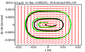
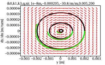
Figure 4: From bottom to top, small, medium, and large betatron amplitude phase space orbits in relativistic self-magnetometer electric storage ring “bottle” with only octupole focusing. Green orbits are CW, black CCW. Focusing parameters and number of turns are shown in the headings. Values of “radial magnetic field error coefficient” $k_{0}$ and number of turns $n$ are chosen just large enough to give visible effect in these graphs. The plots were obtained using MAPLE.

IV Electric Storage Ring Bottle

A quite simple analysis of an idealized relativistic electric storage ring bottle has been given. A real storage ring deviates significantly from this idealization. Perhaps the most significant deviation concerns the effect of the RF cavity necessarily present for bunched beam operation of the storage ring. Even if quite weak, the RF cavity constrains the revolution frequency of every particle to be the same, irrespective of its betatron amplitudes. No such constraint has been included in the analytic formulation given so far. Without the RF, revolution frequencies would depend on betatron amplitudes and fractional momentum offset $\delta$, causing unacceptably small spin coherence time (SCT).

There are other deviations from ideal. Real lattices have straight sections. In the simulations making up the remainder of this paper, the circumference taken up by straight sections is about 15 percent of the total circumference, disributed uniformly. This leaves the ring essentially circular, quite faithful to the analysis so far. The lattice for a real EDM experiment might, more likely, be racetrack shaped. Also the need for polarimeters, octupoles, Wien filters, beam position monitors, injection regions, and diagnostic equipment of various sorts, is likely to require a considerably less symmetric ring, with a smaller fraction of the circumference dedicated to electric bends.

Because the bending elements are discrete, there are end effects in a real storage ring, which have not been considered so far. As it happens, end effects are less serious for orbits than for spin evolution, which is not being considered in this paper. In any case, fringe field effects are included in our simulations and are found to be unimportant.

The simulation code ETEAPOT, which models all-electric rings, has been used. Only a limited simulation of the performance of the relativistic electric bottle has been attempted. Four starting conditions are listed in Table 2, in columns labeled tiny, small, medium, and large amplitude radial, vertical, and fractional momentum offset $\delta$ for the tracked particles. Note that, to limit the number of plots displayed, $x$, $y$, and $\delta$ amplitudes are scaled more or less proportionally—for example, tiny amplitude in, say $x$, and large amplitude in, say $\delta$, is not displayed. Even with this restriction there is an embarrassing proliferation of figures. Furthermore, the same graphs, with the same initial conditions, are repeated later for a magnetic bottle.

The revolution frequency for this ring is $f_{0}=0.6c/281.4=0.6897\,$MHz. Only one (quite low) RF voltage drop $V_{rf}=50\,$keV has been investigated. The RF harmonic number is $h=10$, making $f_{rf}=6.897$MHz. (Much higher harmonic number and lower voltage might be more practical.) These parameters fix the lengths of beam bunches (which can be estimated from the $z$ vs turn number plots).

amplitude	unit	tiny	small	medium	large
$x_{0}$	m	1.0e-5	1.0e-4	0.5e-3	1.0e-3
$x^{\prime}_{0}$		0	0	0	0
$y_{0}$	m	2.0e-5	2.0e-4	1.0e-3	2.0e-3
$y^{\prime}_{0}$		1.0e-7	1.0e-6	0.5e-5	1.0e-5
$\delta$		1.0e-8	1.0e-7	0.5e-6	1.0e-6
$\hat{x}$	cm	0.001	0.01	0.05	0.1
$\hat{y}$	cm	0.05	0.50	2.50	5.0
$Q_{x}$		1.369	1.371	1.369	1.371
$Q_{y}$		0.0091	0.0091	0.0088	0.0090
$Q_{s}$		0.0125	0.0125	0.0118	0.0125

Table 2: Parameter dependencies, ranging from small to large amplitude particles, tracked in electric bottle.

Especially because there are no quadrupoles, nor other linear focusing, the most important question to be established is whether oscillations in all three degrees of freedom are stable. Sinusoidal motion for brief time intervals, i.e. small numbers of turns, provides necessary, though not sufficient, evidence of long time stability. All of the time series graphs, for all amplitudes of all three degrees of freedom, satisfy this test. These are the lower plots in Figures 5 and 6. Note that, to make the sinusoidal oscillations visible, some graphs have been zoomed to show fairly small numbers of oscillations. In all cases the maximum excursions neither shrink nor grow over long times, indicating stability.

A more stringent test of long term stability is exhibited in the upper figures, which provide spectral analyses of the full data sets for the lower figures. The narrow frequency spectra demonstate stability in all cases. Again some of the spectra have been zoomed to permit the line centroids to be determined accurately. The solid vertical lines are centered on these lines, and it is these tunes that are listed as $Q_{x}$, $Q_{y}$, and $Q_{s}$ in Table 2. These are fractional tunes. “Aliasing” suppresses integer tunes. As it happens this affects only $Q_{x}$; its integer tune of 1 has been included in the table.

The broken vertical lines in the tune spectrum plots locate likely nonlinear resonance tunes. In all the plots, only a couple of matches are observed, and they have small amplitudes. This should excuse the absence of explanation of the cryptic (but actually simple) index labels printed above the graphs. Complicating the explanation would be the fact that the alignment of the indices with the broken lines (which are located properly) has been messed up in those plots that have been zoomed.

At even larger amplitudes than are exhibited in these graphs nonlinear resonance proliferate at their expected frequencies and, ultimately, the motion becomes chaotic, limiting the dynamic aperture.

As expected the longitudinal tune $Q_{s}$ is independent of all amplitudes. Dependence of $Q_{x}$ and $Q_{y}$ on amplitude is exhibited by plotting values from the table in Figure 9. The expected constancy of $Q_{x}$ and the strong dependence of $Q_{y}$ on vertical amplitude is observed—$Q_{y}$ is more or less proportional to amplitude. The only important effect of octupole-only focusing is to alter the $Q_{y}$ dependence.

The graphs in Figure 9 also show the corresponding tune dependencies for the purely magnetic storage ring investigated in the next section. With conventional quadrupole focusing both $Q_{x}$ and $Q_{y}$ are independent of betatron amplitudes.

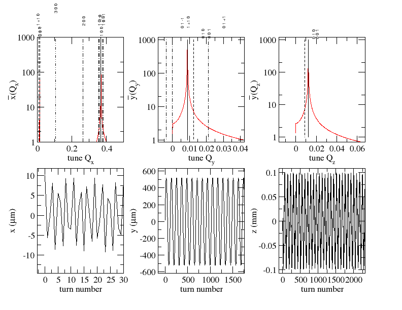
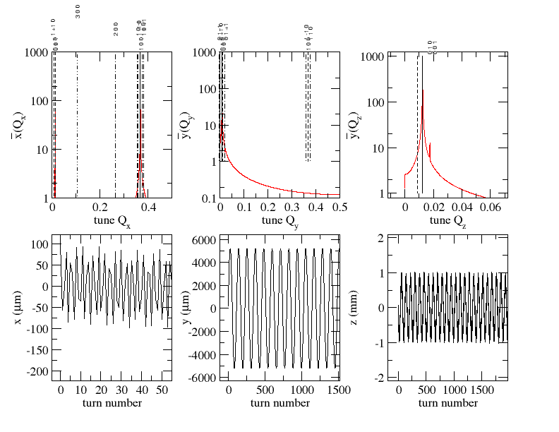
Figure 5: ETEAPOT calculated, electric bottle, $x$, $y$, and $z$ space and frequency domain evolution for “tiny” (above) and “small” amplitude (below). In these and all following spectrum plots, because of aliasing, only fractional tunes are plotted. In every case the integer tune values are 1 for $Q_{x}$ and 0 for $Q_{y}$ and $Q_{z}$.

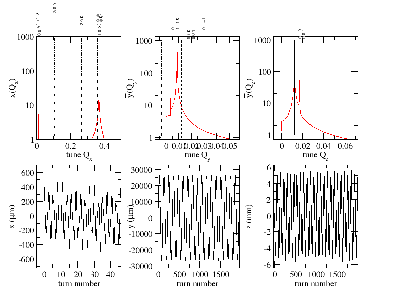
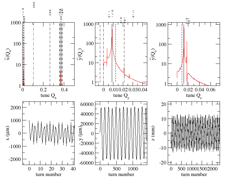
Figure 6: ETEAPOT calculated, electric bottle, $x$, $y$, and $z$ space and frequency domain evolution for “medium” and “large” amplitude.

V Magnetic Storage Ring Bottle

In this section a magnet lattice, differing from the previously discussed electric lattice primarily by the replacement of electric bends by uniform field magnetic bends, is investigated. Like the electric lattice, this lattice would, without vertical focusing, be vertically unstable. In this case, vertical stability is imposed by discrete vertically focusing quadrupoles, situated between bends, and just barely strong enough to provide vertical stability. Tracking is performed using UAL/TEAPOTTEAPOT UAL .

Particles with more or less the same tiny, small, and medium initial amplitudes as in the previous section are tracked, and the results are shown in the same sequence of plots, in Figures 7 and 8. However the “large” amplitude initial conditions that are stable in the electric ring are unstable in the magnetic ring. So the “large” amplitude initial conditions were reduced by a factor of two for the magnetic ring. Even so, insipient nonlinear behavior can be noted, by the proliferation of extra lines in the $Q_{y}$ tune spectrum for the large amplitude case. The small peak identified by the broken line labeled “1 1 0” in the $Q_{y}$ tune plot has a frequency indicating that it is due to nonlinear $(x,y)$ resonance. The stronger peripheral lines are probably also due to nonlinear resonance, but their frequencies are not identified to confirm this.

The magnetic lattice graphs are subject to pretty much the same discussion as for the electric lattice. Amplitudes and tunes extracted from the graphs are entered in Table 3. The dependence of tunes on amplitude are plotted in Figure 9, where they can be compared to the corresponding tunes in the electric ring. Since this is a conventional storage ring both $Q_{x}$ and $Q_{y}$ are constant, independent of amplitude.

amplitude	unit	tiny	small	medium	large
$x_{0}$	m	1.0e-5	1.0e-4	1.0e-3	0.5e-2
$x^{\prime}_{0}$		0	0	0	0
$y_{0}$	m	2.0e-5	2.0e-4	2.0e-3	1.0e-2
$y^{\prime}_{0}$		1.0e-7	1.0e-6	1.0e-5	0.5e-2
$\delta$		1.0e-8	1.0e-7	1.0e-6	0.5e-5
$\hat{x}$	cm	0.001	0.010	0.10	1.0
$\hat{y}$	cm	0.130	0.450	1.55	5.05
$Q_{x}$		1.078	1.080	1.075	1.055
$Q_{y}$		0.0069	0.0226	0.0698	0.159
$Q_{s}$		0.0021	0.0022	0.0020	0.0021

Table 3: Parameter dependencies, ranging from small to large amplitude particles, tracked in magnetic bottle. $Q_{s}$ appears to depend on amplitude, but not outside error bars which are not shown.

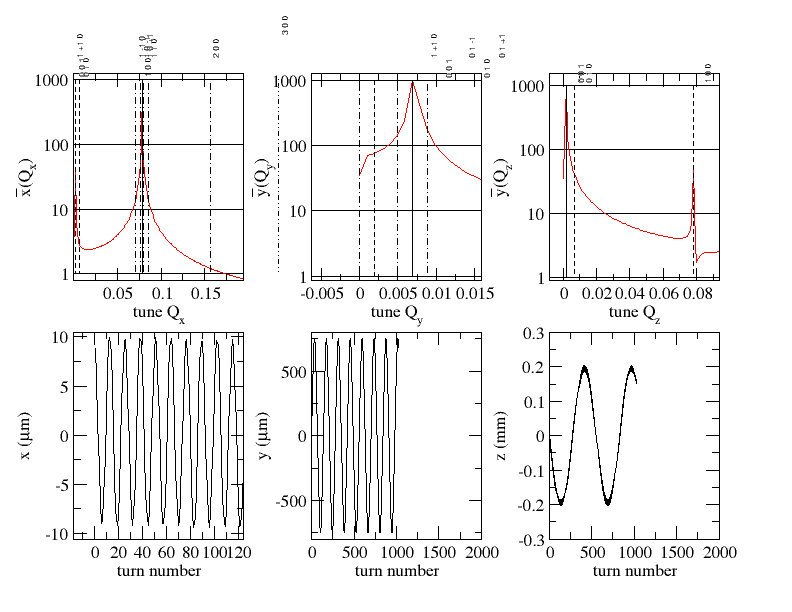
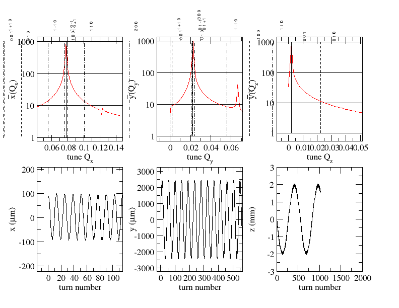
Figure 7: TEAPOT calculated, magnetic bottle, $x$, $y$, and $z$ space and frequency domain evolution for “tiny” (above) and “small” amplitude (below).

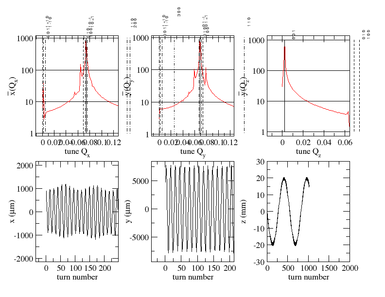
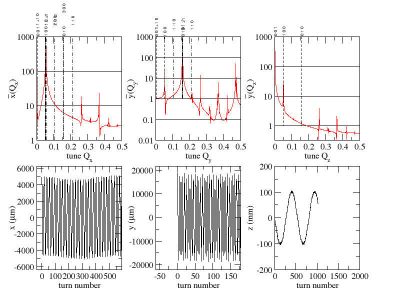
Figure 8: TEAPOT calculated, magnetic bottle, $x$, $y$, and $z$ space and frequency domain evolution for “medium” (above) and “large” amplitude (below).

Figure 9: Horizontal and vertical tunes in electric and magnetic relativistic storage ring bottles. With, at most, very weak explicit quadrupole focusing elements, the horizontal electric ring tune $Q_{x}$ is not far from value 1.28, the pure circular ring theoretical value. For the magnetic ring the horizontal tune $Q_{x}$ is not far from 1.0, the no quadrupole theoretical value. The only strikingly novel feature is the near-linear dependence of $Q_{y}$ on vertical amplitude in the electric case. Of course this is due to the all-octupole focusing.

VI Recapitulation and Conclusions

VI.1 Motivation

The novel relativistic bottles proposed here are more than a curiosity. Especially the electric bottle is appropriate for measuring the electric dipole moments, especially of the proton, but also the electron and other fundamental particles. Because of the proton’s particular anomalous magnetic moment, a polarized proton beam of “magic” 234 MeV kinetic energy, can be “frozen”, meaning that the polarization vector rotates at the same rate, and around the same axis, as the momentum. Out-of-plane tipping of the beam polarization provides the signal basic to the storage ring measurement of the proton EDM. (See referenceBNLproposal .)

EDM measurement relies on measuring the precession caused by the electric field acting on the particle EDM. But the proton MDM is vastly greater than the EDM (whose very existence implies breakdown of both parity and time reversal invariance) for which only upper limits are known. By design $B_{r}=0$ but, inevitably, there will be $\Delta B_{r}$ error fields. The only way to minimize MDM-induced precession is to cancel the magnetic field, primarily by magnetic shielding, secondarily, by cancelling residual magnetic fields by compensation coils.

The achievable EDM accuracy depends on the precision with which the magnetic field can be zeroed. Fortunately it is only the magnetic field averaged over the design orbit that has to be cancelled. Self-magnetometry provides the ideal magnetic measurement for achieving this end. This is because a shift of the beam orbit caused by the unknown magnetic field error, is strictly proportional to the spin precession that needs to be cancelled.

The all-electic case, appropriate only for proton or electron EDM measurement, has been emphasized in this paper. This is the only case where counter-circulating beams can co-exist. However the high-sensitivity magnetometry will be applicable also for rings containing both magnetic and electric bending.

VI.2 Applicability of Electric Bottle

Conventional storage rings rely on quadrupole focusing. This paper has shown how storage rings with only octupole focusing elements will perform much like conventional rings. It is “sefl-magnetometry” that motivates replacing quadrupole focusing by octupole focusing. The electric storage ring bottle with only octupole focusing is ideal for this task. Because the orbit shift to be detected is vertical, it is important for the vertical focusing to be weak—a small vertical force gives a large vertical orbit shift. Relative to this focusing, the geometric horizontal focusing associated with the uniform bending field is strong. As a result, horizontal motion is much the same as in a conventional ring. It is only the vertical focusing that is weak. This contrast is most clearly visible in Figure 9. In particular, unlike in a conventional ring, the vertical tune $Q_{y}$ is roughly proportional to the vertical betatron amplitude.

VI.3 Projected Operational Performance

The performance of an all-electric relativistic storage ring with only octupole focusing has been investigated in Section IV from the point of view of regular storage ring operation. There is satisfactory stability in all three phase space coordinates in spite of the fact that vertical focusing is provided by octupoles rather than quadrupoles. Furthermore, the geometric focusing in the bend elements provides ample horizontal focusing. In short, no quadrupoles (except, perhaps, trim quadrupoles) need to be present in the lattice.

In Section V a quite similar magnetic ring is analysed and found to perform similarly. The Section VII appendix gives a formalism, copied from well known plasma physics theory, for describing a storage ring as a magnetic bottle. The purpose for this appendix is to emphasize that charged particles storage in a “bottle” is not new, and that the nonrelativistic theory can easily be applied to relativistic storage rings.

VI.4 Proton EDM Measurement Options

This section is something of a epilogue, contemplating the experimental implications for the proton EDM measurement that motivated the paper. The main EDM measurement issues were introduced in Section III. The variables are: electron or proton; resonant polarimetry or scattering polarimetry; simultantaneously circulating beams, or one-at-a-time beams? Koop rolling spin wheel or not?; what about the Wien filter directional sensitivity? etc. Far too many for this brief concluding section. Fortunately, other than the essential difference between electron and proton rings, the same lattice designs will be applicable for all choices among the variables. Here I will fix on the proton case, and the two configurations I currently consider most promising.

Though not mentioned so far, and not proven so far, the spin coherence time performance of the octupole-only ring is likely to be superior to any of the rings studied to date. This is because the lattice is closest to the pure $m=0$ cylindrical lattice for which, theoretically, the SCT is infinite. The only blemish needing further study concerns the spin decoherence caused by the (very weak) octupole field.

More important, because the $\langle B_{r}\rangle$ spurious precession is the most serious source of systematic EDM error, the octupole-only bottle storage ring, invented for the purpose, and described in this paper, seems to me to be obligatory. Also for sufficiently high precision, digital frequency domain resonant polarimetry is obligatory. But resonant polarimetry requires the Koop spin wheel rolling polarization, and rolling polarization requires a local Wien filter which, because of its directionality, may rule out simultaneously counter-circulating beams. This seems to reduce the options down to single beams, alternating between CW and CCW runs, with $\langle B_{r}\rangle$ compensation between runs. Aspects of this design have been considered in Section III. This EDM experimental route has the potential for measuring a proton EDM value as small, let us sayFreqDomainEDM , as $10^{-29}\,$e-cm, probably limited by the systematic error caused by spurious MDM-induced precession in unknown residual radial magnetic field.

The only known way to further reduce this systematic error is to have simultaneously counter-circulating beams—an option tentatively ruled out in the italicized sentence in the previous paragraph.

The problem is that controlling the rolling polarization of even a single beam requires two Wien filters. The Wien filter with cancelling horizontal deflections is needed to keep the spin wheel of the polarized beam properly aligned without affecting the orbit at all because the electric and magnetic deflections cancel. But, acting on the counter-circulating beam, the electric and magnetic deflections add. Fortunately even summed, this kick is a mere “tickle”. This Wien filter is only cancelling the spin effects of unknown tiny radial deflections that, nominally, average to zero. Furthermore, any beam growth or change in particle distribution induced in a counter-circulating beam by these kicks is horizontal. As such it has little or no tendency to introduce up-down asymmetry that could influence the EDM measurement. In spite of its directionality, this Wien filter application is therefore probably harmless.

The Wien filter with cancelling vertical electric and magnetic deflections cannot be taken so lightly. The spin kicks from this Wien filter need to be at least strong enough to drive the Koop spin wheel polarization roll, but without influencing the polarized beam orbits. Furthermore, precise reversal of the polarization roll is essential for obtaining the EDM measurement. This spin wheel reversal, if applied by a Wien filter, applies an uncompensated local vertical kick to the counter-circulating beam orbit, possibly producing effects mimicking the effect of particle EDM. This is not good.

I can think of only one way to fix this problem. It is to use the global $\langle B_{r}^{\rm comp}\rangle$ circuit, rather than a local Wien filter, to impose the rolling polarization.

It has been explained in Section III how, working with the $\langle E_{y}^{\rm comp}\rangle$ compensation, the overall radial magnetic field average can be nulled with both beams centered vertically. From this perfectly balanced condition, a tiny shift of $\langle B_{r}^{\rm comp}\rangle$, adiabatically applied, will introduce the required polarization roll. However a tiny vertical beam separation beween the counter-circulating beams will also occur; it is an inevitable consequence of the radial magnetic field driving the roll. This separates the beam centroids everywhere in the ring. But the shift is miniscule and will be treated by correction.

(Vertical separation introduces a small systematic vertical “force” $\Delta f_{y}$ on one beam due to the other but, because the separation is small compared to the beam height, this will not alter the orbits significantly. There will, however, need to be a systematic correction for the MDM-induced spin precession due to the magnetic field of the other beam.)

Otherwise there will be no significant perturbation of either counter-circulating beam distribution. This is because, unlike a local Wien filter, the compensation circuit is global, and varies only adiabatically. For example, half way through each run $\langle B_{r}^{\rm comp}\rangle$ will be slowly reversed as part of the EDM measurement sequence. I conjecture that any spurious systematic EDM signal caused by this sequence of operations can be corrected analytically with satisfactory accuracy.

Another issue to be faced is the “incompatibility” of simultaneously counter-circulating beams with resonant polarimetry (which is itself delicate and, as yet, unproven). The resonant polarimeter is a highly tuned device whose response is only made detectible after millions of coherent bunch passages. The possiblility of separation bumps enabling the beams to pass through separate polarimeters has been contemplated. But this brings in complications too horrible to mention. So I take it as given that both beams have to pass through the same resonators and, in fact, the same everything!

Two beams passing through a single resonator certainly represents a complication. Another complication comes from the fact that each beam has many bunches, presumed to be equally spaced; this is not new, but it is essential to the discussion. To simplify the discussion the rolling spin operation will be turned off for this discussion, returning to truly frozen spin operation, parallel, or anti-parallel to the beam orbits.

Ideally one would wish to monitor and phase lock the beam polarizations of the two beams independently, but this is probably impossible. The beams are injected with independent errors, e.g. different energies, they pass through all the same elements, and there is no significant damping mechanism. The resonator itself cannot distinguish between the beams. Satisfying superposition, the resonator linearly superimposes the signals from all passing bunches, irrespective of their directions of travel. So resonant polarimeters in the ring simply register the coherent sum of the two beam polarizations.

This coherent summing of the two beam polarizations may or may not be tolerable. But, even if not tolerable, there is a workaround. Only one or the other of the CW and CCW beams needs to be polarized for the EDM measurement. An unpolarized beam applies no magnetization signal at all to the polarimeter. So, running with one highly-polarized beam and one unpolarized beam, the polarimeter responds only to the polarized beam, as if there is a single beam. The unpolarized beam is “inert”.

The unpolarized beam provides no EDM information. Its role is to facilitate the self-magnetometry. But it may also be possible for the inert beam to play another role. If the two beam currents are exactly equal (which is not otherwise essential for self-magnetometry) the net current through the magnetometer vanishes. It may be possible to take advantage of this to cancel the direct excitation of the resonator by the circulating beam currents. This would greatly relax one of the serious uncertainties concerning resonant polarimetry. This could, for example, permit the roll polarization frequency to be reduced from, say, 100 Hz to 1 Hz, while still permitting the polarization frequency line to be resolved from the nearby revolution harmonic.

It is not clear whether this will work; direct resonator excitation is more feared than understood at this time. Like the magnetization response, the direct response is also the coherent sum of the responses to the separate beams. The opposite beam directions and the phase shifts through the resonator make it possible for the resonator to be excited even when the net beam current vanishes. By symmetry, arranging the resonator center to coincide with bunch crossing points will probably be either optimal or anti-optimal; i.e. the superposition is either perfectly constructive or perfectly destructive. If anti-optimal, then placing the resonator midway between bunch crossings would be optimal. One only has to design the ring lattice and the RF phasing appropriately.

From this point of view counter-circulating beams may even be helpful for resonant polarimetry. Certainly, this possibility requires further study.

Incidentally, it is already knownBNLproposal , that beam-beam interaction of the counter-circulating beams has negligible detrimental effect on storage ring EDM measurement.

All this implies that simultaneously counter-circulating beams may be practical after all. This route has the potential for reducing the EDM systematic error by a substantial factor—perhaps as much as a factor of ten. This depends on the relative seriousness of unknown radial magnetic fields and the extent to which problems associated with having two beams can be mastered.

APPENDIX

VII Relativistic Magnetic Bottle

This appendix generalizes to relativistic magnetic traps formulas from, for example, a book by SpitzerSpitzer . Results concerning such a relativistic magnetic trap are corroborated in the numerical simulations in Figures 7, 8, and 9.

Some of the formulas in this appendix have been used to include the effects of a very weak magnetic field in an otherwise purely electrostatic field (not counting RF), which is the primary system investigated in the present paper. Behavior of the relativistic all-electric trap emphasized in the present paper is qualitatively very similar to behavior of a magnetic trap.

The dominant field in a magnetic bottle is ${\bf B}=\nabla\times{\bf A}$, where the vector potential ${\bf A}$ is given by

$$\Delta A_{x}=-\frac{1}{2}\,zB,\quad\Delta A_{y}=0,\quad\Delta A_{z}=\frac{1}{2}\,xB.$$ (31)

In the present context “longitudinal” means vertical or $y$, “perpendicular” means horizontal or $(x,z)$. The relativistic Lagrangian for this motion is given by

$$L=-\frac{mc^{2}}{\gamma(v)}-e(\phi-{\bf v}\cdot{\bf A}).$$ (32)

The conjugate momentum vector ${\bf P}$, upper-case to distinguish it from mechanical momentum (lower-case) ${\bf p}$, is defined by

$${\bf P}=\frac{\partial L}{\partial{\bf\dot{v}}}={\bf p}+e{\bf A}.$$ (33)

The Hamiltonian is

$$H={\bf P}\cdot{\bf v}-L=\gamma mc^{2}+e\phi=\sqrt{({\bf P}-e{\bf A})^{2}+m^{2}c^{2}}+e\phi.$$ (34)

In the approximately uniform magnetic field of a magnetic bottle with average value $B$ at the orbit position, with value $B_{0}$ at the center, the particle gyrates around a field line with orbit radius $r=p_{\perp}/(eB)$. The closed line integral $I_{g}$ over one turn,

$$I_{g} =\frac{1}{4\pi}\,\oint{\bf P}_{\perp}\cdot{\bf dl}_{\perp}=\frac{1}{4\pi}\,\oint\Big{(}{\bf p}_{\perp}+e{\bf A}\Big{)}\cdot{\bf dl}_{\perp}$$

$$=\frac{1}{2}\,p_{\perp}r-\frac{1}{4}eB_{0}r^{2}=\frac{1}{4}\,\frac{p^{2}_{\perp}}{eB}.$$ (35)

is an adiabatic invariant of the gyration, conserved as the center of the particle’s circular orbit moves along its field line. The single current orbit loop also has a magnetic moment equal to current times area;

$$\mu_{B}=e\,\frac{v_{\perp}}{2\pi r}\,\pi r^{2}=\frac{1}{2}\,ev_{\perp}r=\frac{1}{2}\,e\frac{p_{\perp}}{m\gamma}\,\frac{p_{\perp}}{eB}=\frac{1}{2}\,\frac{p_{\perp}^{2}}{mB\gamma},$$ (36)

which differs from $I_{g}$ only by a constant factor (which does however include a factor $\gamma$).

$$\mu_{B}=e\,\frac{v_{\perp}}{2\pi r}\,\pi r^{2}=\frac{2}{\gamma}\,I_{g}.$$ (37)

The product $\mu_{B}B=I_{g}B\,2/\gamma$ represents the energy the particle by virtue of its magnetic moment in the magnetic field.

Motion along the field line can be analysed using the constancy of $I_{g}$. Neglecting the longitudinal velocity, the kinetic energy of motion in the perpendicular plane is given by $E_{\perp}=m\gamma c^{2}$. But, because of its initial vertical velocity, a particle will drift vertically. Since the magnetic field is non-uniform this will lead it into a region where $B$ is different. Superficially this seems to contradict the constancy of $I_{g}$, since the speed of a particle cannot change in a pure magnetic field. It has to be that energy is transferred to or from motion in the longitudinal direction. We can analyse the longitudinal motion on the basis of energy conservation.

When the magnitude of $B$ falls with $I_{G}$ constant, the transverse kinetic energy has to increase. This energy necessarily comes from the longitudinal kinetic energy, which falls. Eventually a “turning point” is reached where the longitudinal energy vanishes. and the direction of motion of the guiding center along the field line reverses.

Even though the total velocity is relativistic, for our storage ring application, we can assume the vertical velocity $u_{\parallel}$ can be treated non-relativistically, provided the particle rest mass is replaced by its inertial mass, larger by the factor $\gamma$. For purposes of studying its motion parallel to the magnetic field, the total longitudinal energy of a particle is then given by the non-relativistic formula

$$h=\frac{\gamma}{2}\,I_{g}B(y)+\frac{1}{2}\,m\gamma u^{2}_{\parallel}.$$ (38)

Here $h$ is the numerical value of the total energy (kinetic plus magnetic) of a particular particle being tracked. (The same symbol $h$, with a similar meaning is employed in Section II.3 to express the (non-relativistic) vertical energy of a proton in an electric bottle.) We have specialized from a general case in which the magnetic field depends only on one coordinate $y$, rather than a general position ${\bf R}$. Since the first term depends only on position $y$ it can be interpreted as potential energy. It is larger at either end of the trap than in the middle. Since both $E$ and $I_{g}$ are conserved, this equation can be solved for the dependence of longitudinal velocity on position $y$;

$$u_{\parallel}(y)=\pm\sqrt{\frac{2}{m}\,\Big{(}\frac{h}{\gamma}-\frac{1}{2}\,I_{g}B(y)\Big{)}}.$$ (39)

In a uniform field $u_{\parallel}$ would be constant, but in a spatially variable field $u_{\parallel}$ varies slowly. As the particle drifts toward the end of the trap, the $B$ field becomes stronger and $u_{\parallel}$ becomes less. At some value $y_{\rm tp}$ the right hand side of Eq. (39) vanishes. This is therefore a “turning point” of the motion, and the guiding center is turned back to drift toward the center, and then the other end. Perpetual longitudinal oscillation follows. But the motion may be far from simple harmonic, depending as it does on the detailed shape of ${\bf B}({\bf R})$—for example $B$ can be essentially constant over a long central region and then become rapidly larger over a short end region. (This is the case for the octupole focusing in the all-electric lattice which is the subject of the body of the present paper.)

In any case an adiabatic invariant $I_{\parallel}$ for this motion can be calculated (on-axis) by

$$I_{\parallel}=\frac{1}{2\pi}\,\oint{\bf P}_{\parallel}\cdot\hat{\bf y}\,dy=\frac{m}{2\pi}\,\oint u_{\parallel}dy,$$ (40)

Then the period of oscillation can be calculated from

$$T_{\parallel}=2\pi\,\frac{\partial I_{\parallel}}{\partial h}.$$ (41)

References

- (1) R. Talman, Frequency domain storage ring method for Electric Dipole Moment measurement, arXiv:1508.04366 [physics.acc-ph], 18 Aug 2015
- (2) Storage Ring EDM Collaboration, A Proposal to Measure the Proton Electric Dipole Moment with e-cm Sensitivity, October, 2011
- (3) R. and J. Talman, Symplectic orbit and spin tracking code for all-electric storage rings, Phys. Rev. ST Accel Beams 18, ZD10091, 2015
- (4) N. Malitsky and R. Talman, Accelerator Simulation Using the Unified Accelerator Libraries (UAL,) p. 39, course material available at ”http://uspas.fnal.gov/materials/materials-table.shtml” for USPAS School at Cornell, 2005
- (5) L. Schachinger and R. Talman, TEAPOT: A Thin Element Program for Optics and Tracking, Part. Accel. 22,35(1987)
- (6) N. Malitsky and R. Talman, Unified Accelerator Libraries, Proceedings of Conference on Accelerator Software, Williamsburg, VA, 1996, The Framework of Unified Accelerator Libraries, ICAP98, Monterey, 1998
- (7) R. and J. Talman, Electric Dipole Moment Planning with a resurrected BNL Alternating Gradient Synchrotron electron analog ring, Phys. Rev. ST Accel Beams 18, ZD10092, 2015
- (8) ERXR BPM in “Compact Beam Position Monitor”. Libera Spark Catelog
- (9) I. Podadera, et al., Precision Beam Position Monitor for EUROTEV, Proceedings of DIPAC, Venice, Italy, 2007
- (10) C. Bloomer, et al. Real-time calculation of scale factors of x-ray beam position monitors during user operation, MOPA13, Proc. of IBIC, tskuba, Japan, 2012
- (11) J. Shanks, D.L. Rubin, and D. Sagan, Characterization of the International Linear Collider damping ring optics, arXiv:1309.2248v3 [physics.acc-ph] 4 Sep 2014
- (12) L. Spitzer, Jr., Physics of Fully Ionized Gases, Interscience Publishers, 1956