Effects of the resonant magnetic perturbation on turbulent transport

Abstract

The effects of the resonant magnetic perturbations (RMPs) on the turbulent transport are analyzed in the framework of the test particle approach using a semi-analytical method. The normalized RMP amplitude $P_{b}$ extends on a large range, from the present experiments to ITER conditions. The results are in agreement with the experiments at small $P_{b}.$ The predictions for ITER strongly depend on the type of turbulent transport. A very strong increase of the turbulent transport is obtained in the nonlinear regime, while the effects of the RMPs are much weaker for the quasilinear transport.

Key words: turbulent transport, resonant magnetic perturbations, test particle approach

1 Introduction

The interaction of resonant magnetic perturbations (RMP) with tokamak plasmas determines complex physical precesses that are intensively studied in view of ITER, as seen in the very recent review paper [1]. The goal of suppression or mitigation of the edge localized mode [2], [3] has been achieved in present devices, but there are many aspects that are not understood.

In particular, the studies of the effects of the RMPs on turbulence and transport are in progress. The experiments have clearly shown the increase of turbulence and of the transport in the presence of RMPs in tokamak plasmas [4]-[7] and in other configurations as RFX [8] and LHD [9]. Theoretical models and numerical simulations have confirmed these effects ([10]-[12] and the references there in)

The aim of this paper is to evaluate the direct effects on the RMPs on the turbulent transport as function of the parameters of the turbulence. This is a complementary approach to the selfconsistent numerical simulations, which determine the characteristics of the turbulence and the transport as function of the macroscopic plasma parameters (the gradients, heating, etc.). We present a test particle study, which is expected to bring a different perspective that could contribute to the understanding of the complex interaction process.

The transport regimes for the ions and for the electrons (including multi-scale effects) were recently studied [13], [14]. We determine here, using the same semi-analytical method [15], the effects of the RMPs in each transport regime.

The paper is organized as follows. The model is described in section $2.$ It is a multi-stochastic process determined by the turbulence, the RMPs and particle collisions. The derivation of the statistical solution for the time dependent transport coefficients is presented in Section $3$. We show first that the multi-stochastic process that describe collisional particle transport can be reduced to the transport in stochastic effective velocity field and we determine its Eulerian correlation. The effects of the RMPs on the diffusion coefficients and on the pinch velocity determined by the gradient of the toroidal magnetic field are presented and analyzed in Section $4.$ Section $5$ contains the summary and the conclusions drawn from this work.

2 The model

The test particle approach of transport is based on the evaluation of the Lagrangian velocity correlation (LVC) as a function of the characteristics of the turbulence represented by the Eulerian correlation (EC) or spectrum of the fluctuating potential. The LVC is a time-dependent function $L(t)$ that defines the Lagrangian decorrelation time $\tau_{L}.$ It is the characteristic decay time of the LVC and it measures the statistical memory of the stochastic process. The integral of $L(t)$ is the time dependent diffusion coefficient [16]. The LVC is defined by the statistical average of the trajectories calculated for short times $t\lesssim\tau_{L}.$ The test particle approach can be applied when the typical displacements produced during $\tau,$ which are of the order of the correlation length of the turbulence, are much smaller than the characteristic lengths of the temperature and density [17].

We consider a homogeneous and stationary turbulent plasma represented by a stochastic potential $\phi(\mathbf{x},z,t),$ where $\mathbf{x}=(x,y)$ are the coordinates in the plane perpendicular to the confining magnetic field $B\mathbf{e}_{z}$ (with $x$ in the radial and $y$ in the poloidal directions) and $z$ is the parallel coordinate. The trajectories of the guiding centers are solutions of

$$\frac{d\mathbf{x}}{dt} = -\frac{\mathbf{\nabla}\phi\left(x,y^{\prime},z,t\right)\times\mathbf{e}_{z}}{B}+\dfrac{\mathbf{b}(\mathbf{x},z)}{B}\eta_{\parallel}(t),$$ (1)

$$\frac{dz}{dt} = \eta_{\parallel}(t),$$ (2)

where the first term is the $\mathbf{E}\times\mathbf{B}$ drift, the second term is the velocity determined by the motion along the perturbed magnetic field, $\mathbf{b}(\mathbf{x},z)$ is the perpendicular magnetic field produced by RMP coils, and $\eta_{\parallel}(t)$ is the parallel collisional velocity. The perpendicular collisional velocity is negligible in Eq. (1).

The EC of $\phi,$ which is an input function in test particle studies, is modeled using the results obtained in the numerical simulations for the ion gradient driven turbulence [18]-[20] or for the trapped electron modes [21]. The modes with zero poloidal wave number $k_{y}=0$ are stable for both types of turbulence, which leads to a special shape of the EC that has the poloidal integral equal to zero. The model presented in [13] is used

$$E(\mathbf{x},z,t) \equiv \left\langle\phi(\mathbf{0},0,0)~{}\phi(\mathbf{x},z,t)\right\rangle_{\phi}$$

$$= \Phi^{2}\exp\left(-\frac{x^{2}}{2\lambda_{x}^{2}}-\frac{z^{2}}{2\lambda_{z}^{2}}-\frac{t}{\tau_{c}}\right)\partial_{y^{\prime}}\left[\exp\left(-\frac{y^{\prime\ 2}}{2\lambda_{y}^{2}}\right)y^{\prime}\right],$$

where $\Phi$ is the amplitude of the potential fluctuations, $\lambda_{i},$ $i=x,y,z$ are the correlation lengths along the three directions and $\tau_{c}$ is the correlation time. The derivative $\partial_{y^{\prime}}\equiv\partial/\partial y^{\prime}$ ensure that the poloidal integral is zero. The poloidal drift of the potential with the effective diamagnetic velocity $V_{d}$ is represented by $y^{\prime}=y-V_{d}t$ in Eq. (2). The correlations of the components of the $\mathbf{E}\times\mathbf{B}$ stochastic velocity $v_{i}=-\varepsilon_{ij}\partial_{j}\phi(\mathbf{x},z,t)$ are obtained from the EC of the potential

$$C_{ij}(\mathbf{x},z,t) \equiv \left\langle v_{i}(\mathbf{0},0,0)~{}v_{j}(\mathbf{x},z,t)\right\rangle_{\phi}$$ (4)

$$= -\varepsilon_{ik}\varepsilon_{jl}\partial_{k}\partial_{l}E(\mathbf{x},z,t),$$

where $\varepsilon_{12}=1,$ $\varepsilon_{21}=-1,$ $\varepsilon_{ii}=0,$ $\partial_{1}=\partial/\partial x,$ and $\partial_{2}=\partial/\partial y.$

The confining magnetic field is

$$B(x)=B_{0}\exp\left(-\dfrac{x}{R}\right)\simeq B_{0}\left(1-\dfrac{x}{R}\right),$$ (5)

where $R$ is the major radius of the plasma. The space variation of the confining magnetic field is included in the model through a small gradient in the radial direction, $\mathbf{\nabla}B\simeq B_{0}/R\mathbf{e}_{x}.$

The magnetic perturbations can be resonant (with one dominant mode) or stochastic (with a spectrum of modes of comparable amplitudes) [22]. Considering the averages related to the analysis of the turbulent transport that essentially are space averages over the initial conditions, the magnetic field $\mathbf{b}(\mathbf{x},z)$ contributes to particle trajectories as a stochastic function in both cases. The magnetic field $\mathbf{b}(\mathbf{x},z)$ is represented by a stochastic function that has macroscopic correlation lengths. They are determined by the number and the configuration of the RMP coils and are much larger than the perpendicular correlation length of the turbulence $\lambda_{x},~{}\lambda_{y}$, which are of the order of the ion Larmor radius $\rho_{i}$. Since the trajectories have to be statistically analyzed only for short times that corresponds to displacements at turbulence space scale, the radial and the poloidal variation of $\mathbf{b}(\mathbf{x},z)$ can be neglected. However we take into account the $y$ dependence of $\mathbf{b}$ due to the poloidal component of the unperturbed magnetic field, which determines the rotation of the magnetic lines on the magnetic surfaces and leads to poloidal decorrelation. The toroidal correlation length of $\mathbf{b}$ is smaller than $\lambda_{z},$ which is of the order of $2\pi R$. We also neglect the poloidal component of $\mathbf{b,}$ which is small and is expected to have a weak effect on the radial diffusion coefficient. Thus, the magnetic perturbation is approximated with $\mathbf{b}=b(y,z)\mathbf{e}_{x}.$ The EC of the magnetic field is modeled by

$$C(y,z)\equiv\left\langle b(0,0)~{}b(y,z)\right\rangle_{b}=\beta^{2}\exp\left(-\frac{y^{2}}{2\Lambda_{y}^{2}}--\frac{z^{2}}{2\Lambda_{z}^{2}}\right),$$ (6)

where $\beta$ is the amplitude of the RMPs and $\Lambda_{y},$ $\Lambda_{z}$ are the correlation lengths. They are essentially determined by the number of coils $n$ and $m$ in the toroidal and poloidal directions, respectively

$$\Lambda_{z}=\frac{2\pi R}{n},\ \Lambda_{y}=\frac{\alpha~{}a}{m},$$ (7)

where $a$ is the minor radius and $\alpha$ is the angle of poloidal extension of the coils.

The EC of the collisional velocity $\eta_{\parallel}(t)$ is

$$C_{\parallel}(t)=\left\langle\eta_{\parallel}(0)\eta_{\parallel}(t)\right\rangle_{\parallel}=\chi_{\parallel}\nu~{}\exp(-\nu\left|t\right|),$$ (8)

where $\nu$ is the frequency of collisions, $\chi_{\parallel}=\lambda_{mfp}^{2}\nu$ is the parallel diffusivity, $\lambda_{mfp}$ is the mean free path, and $\left\langle{}\right\rangle_{\parallel}$ is the statistical average.

Dimensionless variables are introduced. The perpendicular displacements, the correlation lengths ($\lambda_{x},$ $\lambda_{y},$ $\Lambda_{y})$ and the gradient length $R$ are normalized with the ion Larmor radius $\rho_{i}$. The parallel displacements $z,$ $\lambda_{z},$ $\Lambda_{z}$ are divided by $L_{T_{i}},$ the gradient length of the ion temperature $T_{i}$. The unit of time and of $\tau_{c}$ is $\tau_{0}=L_{T_{i}}/v_{T_{i}},$ where $v_{T_{i}}=\sqrt{T_{i}/m_{i}}$ is the thermal velocity of the ions and $m_{i}$ is their mass. The collisional velocity is normalized with the amplitude $\sqrt{\chi_{\parallel}\nu}=v_{T_{i}}.$ The units for potential and for the magnetic field are $\Phi$ and $\beta,$ respectively. Using the same symbols for the dimensionless variables, the equations of motion in the reference system that moves with the potential are

$$\frac{dx}{dt} = -P_{\phi}\exp(\frac{x}{\overline{R}})\mathbf{~{}\partial}_{y}\phi\left(x,y,z,t\right)+P_{b}\exp(\frac{x}{\overline{R}})b(y,z)\eta_{\parallel}(t)$$ (9)

$$\frac{dy}{dt} = P_{\phi}\exp(\frac{x}{\overline{R}})\mathbf{~{}\partial}_{x}\phi\left(x,y,z,t\right)+\overline{V}_{d}$$ (10)

$$\frac{dz}{dt} = \eta_{\parallel}(t)$$ (11)

where $\overline{V}_{d}=V_{d}/V_{\ast}$ with the diamagnetic velocity $V_{\ast}=\rho_{i}~{}v_{T_{i}}/L_{T_{i}}.$ All the stochastic fields in Eqs. (9-11) have the amplitudes equal to one. The correlation function of the normalized collisional velocity is

$$C_{\parallel}(t)=\exp(-P_{c}\left|t\right|).$$ (12)

Three dimensionless parameters appear in the normalized equations (9-11)

$$P_{\phi}\equiv\frac{\Phi}{B_{0}\rho_{i}V_{\ast}}=\frac{e\Phi}{T_{i}}\frac{L_{T_{i}}}{\rho_{i}},$$ (13)

$$P_{b}\equiv\frac{\beta~{}v_{T_{i}}}{B_{0}V_{\ast}}=\frac{\beta}{B_{0}}\frac{L_{T_{i}}}{\rho_{i}},$$ (14)

$$P_{c}\equiv\frac{\rho_{i}~{}\nu}{V_{\ast}}=\frac{L_{T_{i}}}{\lambda_{mfp}},$$ (15)

where $\lambda_{mfp}=v_{T_{i}}/\nu.$ These parameters measure the influence that the three stochastic processes (turbulence, RMPs and particle collisions) have on particle motion. The stochastic functions are statistically independent, but a strong nonlinear interaction can appear through particle trajectories due to the space dependence of $\phi$ and $b$.

3 The semi-analytical solution

The perpendicular diffusion coefficient is determined as function of $P_{\phi},$ $P_{b},$ $P_{c},$ $\overline{R}$ and $\tau_{c}.$ The space dependence of potential makes the transport strongly nonlinear. Nonlinear effects of the RMPs are expected when $P_{\phi}/P_{b}$ is large. In these conditions the particles can explore the structure of the stochastic potential before they leave the correlated zone due to magnetic line displacements.

A semi-analytical approach based on the decorrelation trajectory method (DTM, [15]) is developed for this multi-stochastic process.

The change of variable from $\mathbf{x}$  to $\mathbf{x}^{\prime}=\mathbf{x-}x_{b}(t)\mathbf{e}_{x},$ where $x_{b}(t)$ is the displacement produced by the RMPs, permits to define an effective velocity that includes the three stochastic functions

$$\mathbf{v}^{eff}(\mathbf{x}^{\prime},t)=-\exp\left(\frac{x^{\prime}+x_{b}(t)}{\overline{R}}\right)\mathbf{\nabla}^{\prime}\phi(\mathbf{x}^{\prime}+x_{b}(t)\mathbf{e}_{x},z(t),t)\times\mathbf{e}_{z}.$$ (16)

The equations of motion in this frame is

$$\frac{d\mathbf{x}^{\prime}}{dt}=P_{\phi}\,\mathbf{v}_{eff}(\mathbf{x}^{\prime},t)+V_{d}\mathbf{e}_{y}.$$ (17)

The transport formally appears in Eq. (17) as produced by a single stochastic velocity. This is an important simplification, which is effective if the EC of $\mathbf{v}^{eff}(\mathbf{x}^{\prime},t)$ can be estimated. The latter is defined as the average over all of the stochastic processes

$$E_{ij}^{eff}(\mathbf{x}^{\prime},t)=\left\langle\left\langle\left\langle v_{i}^{eff}(\mathbf{0},0)\ v_{j}^{eff}(\mathbf{x}^{\prime},t)\right\rangle_{\phi}\right\rangle_{\parallel}\right\rangle_{b}.$$ (18)

The steps for determining the semi-analytical solution of this transport problem are presented below. The statistic of the parallel collisional motion is determined in Subsection 3.1. The probability of the displacements $x_{b}(t)$ induced by the RMPs is analyzed in 3.2. The EC of the effective velocity (18) is calculated in Subsection 3.3 and a short review of the DTM for determining the time dependent diffusion coefficients is presented in 3.4.

3.1 Parallel collisional transport

The first step consists of determining the $z$ component of the trajectories from Eq. (11). This is a well known linear stochastic process that leads to Gaussian distribution of the trajectories $z(t).$ We give here the results which are necessary for the following calculations. The probability that the trajectories are in $z$ at time $t$ is

$$P_{\parallel}(z,t)\equiv\left\langle\delta\left(z-z(t)\right)\right\rangle_{\parallel}=\frac{1}{\sqrt{2\pi\left\langle z^{2}(t)\right\rangle_{\parallel}}}\exp\left(-\frac{z^{2}}{2\left\langle z^{2}(t)\right\rangle_{\parallel}}\right),$$ (19)

where the mean square displacement (MSD) is

$$\left\langle z^{2}(t)\right\rangle_{\parallel}=2\int_{0}^{t}d_{\parallel}(\tau)~{}d\tau=2P_{c}^{-2}\left[P_{c}t+\exp(-P_{c}t)-1\right]$$ (20)

and

$$d_{\parallel}(t)=\int_{0}^{t}C_{\parallel}(\tau)~{}d\tau=P_{c}^{-1}\left[1-\exp(-P_{c}t)\right].$$ (21)

is the time dependent diffusion coefficient along the magnetic field lines.

3.2 Transport induced by RMPs

The displacements produced by the RMPs are solutions of

$$\frac{dx_{b}}{dt}=P_{b}\exp(\frac{x^{\prime}+x_{b}}{\overline{R}})b(y,z)\eta_{\parallel}(t),\ \ \frac{dz}{dt}=\eta_{\parallel}(t).$$ (22)

We consider first a constant confining magnetic field $(\overline{R}\rightarrow\infty)$

$$\frac{dx_{0}}{dt}=P_{b}b(y,z(t))\eta_{\parallel}(t).$$ (23)

The velocity in the right hand side of this equation is the product of two stochastic functions, the magnetic field and the collisional velocity. Its Lagrangian correlation is defined by

$$C_{v}\equiv\left\langle\left\langle b(0,0)\ b(y,z(t))\right\rangle_{b}\eta_{\parallel}(0)\eta_{\parallel}(t)\right\rangle_{\parallel}.$$ (24)

The poloidal confining magnetic field $B_{p}$ leads to the poloidal rotation of the magnetic lines, which are at the angle $\iota$ with the $z$ axis, where $tg(\iota)=B_{p}/B_{0}.$ The collisional particle motion along the magnetic lines $\zeta(t)$ has projections in the toroidal $z(t)=\zeta(t)\cos(\iota)$ and poloidal $y(t)=\zeta(t)\sin(\iota)$ directions. Since $\iota$ is small $z(t)\cong\zeta(t),$ $y(t)\cong\zeta(t)B_{p}/B_{0}\cong z(t)B_{p}/B_{0}.$ Using Eq. (6) one obtains

$$C_{v}\equiv\left\langle\exp\left(-\frac{z^{2}(t)}{2\Lambda_{eff}^{2}}\right)\eta_{\parallel}(0)\eta_{\parallel}(t)\right\rangle_{\parallel},$$ (25)

where

$$\Lambda_{eff}=\frac{\Lambda_{z}}{\sqrt{1+\left(\frac{\Lambda_{z}}{\Lambda_{y}}\frac{B_{p}}{B_{0}}\right)^{2}}}.$$ (26)

This shows that the finite $\Lambda_{y}$ of the RMPs determines an effective correlation length, which is smaller than $\Lambda_{z}.$ The factor in Eq. (26) depends on the number of coils and it is of the order $\sqrt{1+(m/qn)^{2}},$ where $q$ is the safety factor.

The correlation in Eq. (25) is written using $\delta$-function to impose the condition $z(t)=z$

$$C_{v} = \int_{-\infty}^{\infty}dz~{}\exp\left(-\frac{z^{2}}{2\Lambda_{eff}^{2}}\right)\left\langle\delta(z-z(t))~{}\eta_{\parallel}(0)\eta_{\parallel}(t)\right\rangle_{\parallel}$$

$$= \frac{1}{2\pi}\int\int_{-\infty}^{\infty}dz~{}dq\exp\left(-\frac{z^{2}}{2\Lambda_{eff}^{2}}+iqz\right)\left\langle\exp(-qz(t))~{}\eta_{\parallel}(0)\eta_{\parallel}(t)\right\rangle_{\parallel}$$

The average in this equation is

$$M_{\parallel} \equiv \left\langle\exp\left(-iqz(t)\right)~{}\eta_{\parallel}(0)\eta_{\parallel}(t)\right\rangle_{\parallel}$$ (28)

$$= \frac{1}{q^{2}}\partial_{t}\partial_{t_{0}}\left.\left\langle\exp\left(-iq\int_{t_{0}}^{t}d\tau~{}\eta_{\parallel}(\tau)\right)\right\rangle_{\parallel}\right|_{t_{0}=0}.$$

Since $\eta_{\parallel}$ and $z(t)$ are Gaussian functions, the average of the exponential is

$$\exp\left(-\frac{q^{2}}{2}\int_{t_{0}}^{t}d\tau\int_{t_{0}}^{t}d\tau^{\prime}~{}C_{\parallel}(\left|\tau-\tau^{\prime}\right|)\right).$$ (29)

Straightforward calculations lead to

$$M_{\parallel}=\left(C_{\parallel}(t)-q^{2}d_{\parallel}^{2}(t)\right)\exp\left(-\frac{q^{2}}{2}\left\langle z^{2}(t)\right\rangle_{\parallel}\right).$$ (30)

The LVC of the RMP (3.2) becomes after calculating the integrals

$$C_{v}(t)=P_{b}^{2}\frac{\Lambda_{eff}~{}\left[C_{\parallel}(t)(\Lambda_{eff}^{2}+\left\langle z^{2}(t)\right\rangle_{\parallel})-d_{\parallel}^{2}(t)\right]}{(\Lambda_{eff}^{2}+\left\langle z^{2}(t)\right\rangle_{\parallel})^{3/2}}.$$ (31)

The time integral of this function gives the time dependent diffusion coefficient generated by RMPs

$$D_{b}(t)=P_{b}^{2}\Lambda_{eff}~{}\frac{d_{\parallel}^{2}(t)}{(\Lambda_{eff}^{2}+\left\langle z^{2}(t)\right\rangle_{\parallel})^{1/2}}.$$ (32)

The MSD is obtained by integrating once more

$$\left\langle x_{0}^{2}(t)\right\rangle_{b\parallel}=2P_{b}^{2}\Lambda_{eff}~{}\left((\Lambda_{eff}^{2}+\left\langle z^{2}(t)\right\rangle_{\parallel})^{1/2}-\Lambda_{eff}\right)$$ (33)

This is the well known [23] process of subdiffusive transport of the double diffusion type (magnetic field line diffusion combined with the collisional particle diffusion along field lines). It corresponds to the quasilinear transport in stochastic magnetic fields. Nonlinear effects appear for space dependent magnetic fields with large Kubo numbers [24].

Any perturbation that lead to the departure of the particles from the field lines leads to diffusive particle transport. Such a perturbation can be the collisional perpendicular velocity, plasma rotation or even the small magnetic drifts determined by the curvature of the magnetic lines. In the process studied here, the $\mathbf{E}\times\mathbf{B}$ stochastic velocity produces the strongest decorrelation effect and it has the main role in determining the RMP diffusion coefficient. However, since the correlation lengths of $\mathbf{b}$ are very large (at macroscopic scale), the characteristic time $\tau_{b}$ for the saturation of $D_{b}(t)$ is large. It is much larger than the Lagrangian characteristic time of the turbulence $\tau_{b}>>\tau_{L}.$ Thus, the RMP transport process can be approximated by Eq. (32)-(33) during $\tau_{L}.$ The turbulence and other decorrelation mechanisms have negligible effects at such small times.

We note that the complex structure of the magnetic field lines generated by the RMPs (see for instance [1]) does not influence the transport process studied here. The magnetic structure with stochastic regions and island chains is evidenced by following the magnetic lines for many toroidal rotations. Or, the turbulence has a parallel correlation length of the order of $\overline{R},$ which means that after one toroidal rotation the particles leave the magnetic lines. In other words, the particles do not ”see” the complex structure of the magnetic lines in the presence of turbulence.

We evaluate now the effect of the gradient of the confining magnetic field taking into account the $\overline{R}$ dependent factor in Eq. (22). It can be written as

$$\frac{dx_{b}}{dt}=P_{b}\exp(\frac{x^{\prime}+x_{b}}{\overline{R}})\frac{dx_{0}}{dt}.$$ (34)

The solution in terms of $x_{0}(t)$ is

$$x_{b}(t) = -\overline{R}~{}\ln\left(1-\frac{x_{0}(t)}{\overline{R}}\exp\left(\frac{x^{\prime}}{\overline{R}}\right)\right)$$

$$\cong x_{0}(t)\exp\left(\frac{x^{\prime}}{\overline{R}}\right)+\frac{x_{0}^{2}(t)}{2\overline{R}}\exp\left(\frac{2x^{\prime}}{\overline{R}}\right)+\frac{x_{0}^{3}(t)}{3\overline{R}^{2}}\exp\left(\frac{3x^{\prime}}{\overline{R}}\right)+...$$

The average of this equation is

$$\left\langle x_{b}(t)\right\rangle\cong\frac{\left\langle x_{0}^{2}(t)\right\rangle}{2\overline{R}}\exp\left(\frac{2x^{\prime}}{\overline{R}}\right)\cong\frac{\left\langle x_{0}^{2}(t)\right\rangle}{2\overline{R}},$$ (36)

and the average of the square is

$$\left\langle x_{b}^{2}(t)\right\rangle\cong\left\langle x_{0}^{2}(t)\right\rangle\exp\left(\frac{2x^{\prime}}{\overline{R}}\right),$$ (37)

where the linear approximation in the small parameter $1/\overline{R}$ was taken.

The probability of the RMP generated displacements is Gaussian in the linear approximation in $1/\overline{R}$

$$P_{b}(x_{b},t)\cong\frac{1}{\sqrt{2\pi\left\langle x_{b}^{2}(t)\right\rangle}}\exp\left(-\frac{\left(x_{b}-\left\langle x_{b}(t)\right\rangle\right)^{2}}{2\left\langle x_{b}^{2}(t)\right\rangle}\right)$$ (38)

Thus, the gradient of the confining magnetic field generates an average displacement that is proportional to the MSD produced by the RMPs, and to the gradient. Such average displacement generates an average velocity (direct transport)

$$V_{b}(t)\equiv\frac{d\left\langle x_{b}(t)\right\rangle}{dt}=\dfrac{D_{b}(t)}{\overline{R}}~{}$$ (39)

The velocity $V_{b}$ is positive, directed against the gradient of the magnetic field, towards plasma boundary. It is transitory for the subdiffusive transport, and a finite asymptotic value exists only in the presence of a process of decorrelation of the particles from the field lines. We are interested here in the nonlinear effects produced by the average displacement $\left\langle x_{b}(t)\right\rangle$ on the turbulent transport.

3.3 The EC of the effective velocity

The averages over the three stochastic functions that appear in the effective velocity are calculated according to the definition (18).

The average over the stochastic potential yields the EC of the $\mathbf{E}\times\mathbf{B}$ drift components (4)

$$M_{ij} \equiv \left\langle v_{i}^{eff}(\mathbf{0},0)\ v_{i}^{eff}(\mathbf{x}^{\prime},t)\right\rangle_{\phi}$$

$$= C_{ij}(\mathbf{x}^{\prime}+x_{b}(t)\mathbf{e}_{x},z(t),t)~{}\exp\left(\frac{x^{\prime}+x_{b}(t)}{\overline{R}}\right).$$

The average over the parallel collisional velocity $\eta_{\parallel}(t)$ is obtained using the probability (19) of $z(t)$. It applies in the case of the EC (2) only to the $z$ dependent factor, which becomes

$$\left\langle\exp\left(-\frac{z^{2}}{2\lambda_{z}^{2}}\right)\right\rangle_{\parallel} = \int_{-\infty}^{\infty}\exp\left(-\frac{z^{2}}{2\lambda_{z}^{2}}\right)P_{\parallel}(z,t)dz$$ (41)

$$= \frac{\lambda_{z}}{\sqrt{\lambda_{z}^{2}+\left\langle z^{2}(t)\right\rangle_{\parallel}}}.$$

The average over the RMPs is calculated using the probability (38) of the magnetic displacements. This average changes only the radial factor in the EC (2) multiplied by the gradient of the confining magnetic field, which is

$$M_{b} \equiv \left\langle\exp\left(-\frac{(x^{\prime}+x_{b}(t))^{2}}{2\lambda_{x}^{2}}\right)\exp\left(\frac{x^{\prime}+x_{b}(t)}{\overline{R}}\right)\right\rangle_{b}$$

$$= \int_{-\infty}^{\infty}\exp\left(-\frac{(x+x_{b})^{2}}{2\lambda_{x}^{2}}+\frac{x^{\prime}+x_{b}}{\overline{R}}\right)P_{b}(x_{b},t)dx_{b}$$

One obtains after neglecting a small term of second order in $1/\overline{R}$

$$M_{b} = \frac{\lambda_{x}}{\sqrt{\lambda_{x}^{2}+\left\langle x_{b}^{2}(t)\right\rangle}}\exp\left[-\frac{(x^{\prime}+\left\langle x_{b}(t)\right\rangle)^{2}}{2(\lambda_{x}^{2}+\left\langle x_{b}^{2}(t)\right\rangle)}\right]$$ (42)

$$\exp\left(\frac{x^{\prime}+\left\langle x_{b}(t)\right\rangle}{\overline{R}}\frac{\lambda_{x}^{2}}{\lambda_{x}^{2}+\left\langle x_{b}^{2}(t)\right\rangle}\right).$$

Finally, the EC of the effective velocity (18) can be written as

$$E_{ij}^{eff}(\mathbf{x}^{\prime},t)=-\varepsilon_{ik}\varepsilon_{jl}\partial_{k}\partial_{l}\left[E^{eff}(\mathbf{x}^{\prime},t)\right]\exp\left(\frac{x^{\prime}+\left\langle x_{b}(t)\right\rangle}{R^{eff}}\right),$$ (43)

where

$$E^{eff}(\mathbf{x}^{\prime},t)=\frac{\lambda_{x}}{\lambda_{x}^{eff}}\frac{\lambda_{z}}{\lambda_{z}^{eff}}\exp\left(-\frac{(x^{\prime}+\left\langle x_{b}(t)\right\rangle)^{2}}{2(\lambda_{x}^{eff})^{2}}\right)\partial_{y}\left(\exp\left(-\frac{y^{2}}{2\lambda_{y}^{2}}\right)y\right),$$ (44)

$$\lambda_{x}^{eff}(t)=\sqrt{\lambda_{x}^{2}+\left\langle x_{b}^{2}(t)\right\rangle},$$ (45)

$$R^{eff}=\overline{R}\frac{\left(\lambda_{x}^{eff}\right)^{2}}{\lambda_{x}^{2}},$$ (46)

$$\lambda_{z}^{eff}(t)=\sqrt{\lambda_{z}^{2}+\left\langle z^{2}(t)\right\rangle_{\parallel}}.$$ (47)

The last factor in Eq. (43) is determined by the gradient of the confining magnetic field, and the other have the same structure as in Eq. (4), which relates the correlation of the drift velocity to the EC of the potential. An effective potential with the EC (44) can be defined for $\mathbf{v}^{eff}(\mathbf{x}^{\prime},t).$

The difference between the effective velocity and the $\mathbf{E}\times\mathbf{B}$ drift velocity consists of the change of the EC of the potential. Comparing Eq. (44) with Eq. (2), one can see that the modification concern the radial dependence of the EC. It consists of the shift of the maximum with the average displacement generated by the RMPs and of the increase of the correlation length, which becomes a time-dependent function (45). The RMPs also determine the decay in time of the amplitude as $\lambda_{x}/\lambda_{x}^{eff}(t).$

The parallel motion eliminates the $z$ dependent factor in (2) and leads to the time decay of the amplitude of the effective potential as $\lambda_{z}/\lambda_{z}^{eff}(t).$ the exponential decay with $z$ is transformed into a slow decorrelation (the decay of the amplitude as $1/\sqrt{t}).$ The parallel collisional velocity also determines the subdiffusive behaviour of the MSD of the RMP displacements $x_{b}(t).$ This effect leads to a slow decorrelation of $\mathbf{v}^{eff}$ in the radial direction, much slower than in the absence of parallel collisions when the RMP radial transport is diffusive.

The factor determined by the gradient of the toroidal magnetic field in Eq. (43) is modified by the RMPs, which determine a shift of the maximum and the increase of the gradient length (46). This means that the effect of $\overline{R}$ decreases in time.

3.4 The DTM

The multi-stochastic process that describes turbulent transport in the presence of RMPs was reduced to the problem of 2-dimensional transport in an effective velocity field that has the EC (43) with $E^{eff}(\mathbf{x}^{\prime},t)$ given by (44).

We use the DTM [15] for determining the time dependent diffusion coefficient. This method is based on a set of deterministic trajectories, the decorrelation trajectories (DTs), which are obtained from the EC of the effective velocity. We define a set of subensembles $S$ with given values of the stochastic functions at the origin:

$$\phi^{eff}(\mathbf{0},0)=\phi^{0},\quad\mathbf{v}^{eff}(\mathbf{0},0)=\mathbf{v}^{0}.$$ (48)

The effective velocity is in each subensemble S is a Gaussian field with the average

$$V_{i}^{S}(\mathbf{x},t)=\phi^{0}E_{\phi i}^{eff}(\mathbf{x}^{\prime},t)+v_{1}^{0}E_{1i}^{eff}(\mathbf{x}^{\prime},t)+v_{2}^{0}E_{2i}^{eff}(\mathbf{x}^{\prime},t),$$ (49)

where $E_{\phi i}^{eff}(\mathbf{x}^{\prime},t)=-\varepsilon_{ik}\partial_{k}E^{eff}(\mathbf{x}^{\prime},t)$ are the correlations of the potential with the effective velocity. The DTs are approximate average trajectories in the subensembles obtained by solving the equation

$$\frac{d\mathbf{X}^{S}(t)}{dt}=P_{\phi}\mathbf{V}^{S}(\mathbf{X}^{S}(t),t)\exp\left(\frac{X^{S}(t)+\left\langle x_{b}(t)\right\rangle}{R^{eff}}\right)+V_{d}\mathbf{e}_{y}.$$ (50)

The fluctuations of the trajectories are neglected in this equation. This approximation is supported by the high degree of similarity of the trajectories in a subensemble, which is determined by the supplementary initial conditions (48), and by the small small amplitude of the velocity fluctuations in a subensemble [25].

The time dependent diffusion coefficient and the average radial displacement are obtained by summing the contributions of all subensembles (see [15] for details)

$$D_{i}(t)=\int d\phi^{0}d\mathbf{v}^{0}P(\phi^{0})P(\mathbf{v}^{0})~{}v_{i}^{0}X_{i}^{S}(t),$$ (51)

$$\left\langle x(t)\right\rangle=\int d\phi^{0}d\mathbf{v}^{0}P(\phi^{0})P(\mathbf{v}^{0})~{}X_{i}^{S}(t).$$ (52)

The direct contribution of the transport produced by the RMPs has to be added. Thus the diffusion coefficients in physical units are

$$D_{i}^{tot}(t;P_{\phi},P_{b},P_{c},\overline{R})=\frac{\Phi}{B_{0}}\left(D_{i}(t;P_{\phi},P_{b},P_{c},\overline{R})+D_{b}(t;P_{b},P_{c},\overline{R})\right)$$ (53)

The asymptotic diffusion coefficients are

$$\chi_{i}^{tot}(P_{\phi},P_{b},P_{c},\overline{R})=\frac{\Phi}{B_{0}}\left(\chi_{i}(P_{\phi},P_{b},P_{c},\overline{R})+\chi_{b}(P_{b},P_{c},\overline{R})\right),$$ (54)

Thus, the diffusion coefficients $D_{i}^{b}(t)$ are obtained from Eq. (51) using the solutions of Eq. (50) for the DTs. The latter have to be numerically calculated, although they are very simple. A computer code was developed for the calculation of the decorrelation trajectories, of the running diffusion coefficient (51) and of the average displacement (52). The numerical calculations are at the microcomputer level with runs of the order of few minutes.

4 The effects of RMPs on turbulent transport

We analyze here the effects of the RMPs on transport as function of turbulence parameters. The effects produced by the increase of RMP intensity on turbulence are not considered. The aim is to identify the direct change of transport.

The multi-stochastic process that describes the turbulent transport in the presence of RMPs depends on twelve physical parameters. This number is reduce to 10 using dimensionless variables. This large number of parameters imposes a first analysis of their ranges and of the importance of each term before quantitative evaluations.

The main parameters are $P_{\phi}$ (13) and $P_{b}$ (14), the amplitudes of the turbulence and of the RMPs, respectively. We consider ion temperature (ITG) driven turbulence that has correlation lengths of the order of $\rho_{i}.$ The values taken in the figures are $\overline{\lambda}_{x}\equiv\lambda_{x}/\rho_{i}=4$ and $\overline{\lambda}_{y}\equiv\lambda_{y}/\rho_{i}=2.$ The parallel correlation length $\lambda_{z}$ is of the order of $R,$ which leads to $\overline{\lambda}_{z}\equiv\lambda_{z}/L_{T_{i}}=\overline{R}/L_{T_{i}},$ which is of the order of the ITG parameter. A value that corresponds to well developed ITG turbulence is taken for the calculations in the figures ($\overline{\lambda}_{z}=6$ ). The drift velocity $V_{d}$ is of the order of the diamagnetic velocity, which leads to $\overline{V}_{d}\lesssim 1.$ Thus, the analysis of the dependence of the transport on four of the parameters of the model is not necessary since they have narrow variation range and determine weak effects. Also, the collision parameter $P_{c}$ (15) has a weaker effect. It essentially separates the ballistic and the diffusive behavior of the parallel trajectories and influences the MSD of the displacements produced by the RMPs.

The normalized amplitude of the RMPs can be written as

$$P_{b}=(\beta/B_{0})(L_{T_{i}}/R)(R/a)(a/\rho_{i})\simeq 0.5(\beta/B_{0})(a/\rho_{i}).$$ (55a)

It depends on the amplitude of the magnetic field and on plasma size. Its values are $$P_{b}\lesssim 1 P_{b}\simeq 10 \left[0.01,~{}100\right].$$ in the actual experimental conditions and will increase to for ITER. The effects of the RMPs on turbulent transport are analyzed for a large range of amplitudes

We begin by a short presentation of the trapping process and of the transport regimes obtained in a turbulence with the EC of the type (2) in the absence of the RMPs (Subsection 4.1). The effects of the RMPs on the transport and on the turbulent pinch determined by the gradient of the toroidal magnetic field are discussed in 4.2.

4.1 Trajectory trapping      

Particle trajectories in turbulent plasmas can have both random and quasi-coherent aspects. A typical trajectory is a random sequence of long jumps and trapping events that consists of winding on almost closed paths. Trapping introduces quasi-coherent aspects in trajectory statistics. It determines a large degree of coherence in the sense that bundles of trajectories that start from neighboring points remain close for very long time compared to the eddying time [25]. This process generates intermittent, quasi-coherent structures of trajectories similar to fluid vortices.

A strong interdependence exists between ion trajectory statistics and the evolution of the drift type turbulence. This interaction is rather complex and it involves both the random and the quasi-coherent aspects, but with completely different effects. Trajectory diffusion has a stabilizing effect on turbulence [26] while trajectory trapping leads to strong nonlinear effects [27]. The strength of each of these processes depends on the stage in the evolution of turbulence. The transport is related to the stochastic aspect of trajectories, and trajectory structures have a hindering effect. The trapped particle do not contribute to transport, but they represent a reservoir of transport. Any perturbation that liberates particles leads to increased transport and to anomalous transport regimes.

The turbulent transport in the absence of RMPs ($P_{b}=0)$ was studied in [13] for a potential with EC of the type (2). We present here a short review of these results and of their physical image.

The process is nonlinear due to the $\mathbf{x}$ dependence of the stochastic potential. The nonlinearity manifests as trajectory trapping or eddying due to the Hamiltonian structure of Eqs. (9-10), which lead to the invariance of the Lagrangian potential for $\tau_{c}\rightarrow\infty,$ $\lambda_{z}\rightarrow\infty$ and $V_{d}=0.$ The trajectories remain on the contour lines of the potential, and the transport is subdiffusive in these conditions. The time variation of the potential and/or particle parallel motion when $\lambda_{z}$ is finite represent decorrelation mechanisms, which lead to finite asymptotic values of the diffusion coefficient. Depending on the strength of these perturbations, represented by decorrelation characteristic times $\tau_{d}$, trajectory trapping is partially or completely eliminated. The condition for the existence of trapped trajectories is $\tau_{d}>\tau_{fl},$ where $\tau_{d}\equiv\tau_{c}\tau_{z}/(\tau_{c}+\tau_{z}),$ $\tau_{z}$ is the parallel decorrelation time, and $\tau_{fl}=\lambda_{x}/V_{x}+\lambda_{y}/V_{y}$ is the time of flight of the particles or the eddying time. The average velocity $V_{d}$ also influences the trapping, but in a different way. It determines an average potential $xV_{d}$ that adds to the stochastic potential $\phi(\mathbf{x}).$ The total potential has a strongly modified structure. Bunches of open contour lines between islands of closed lines appear for small $V_{d}$ ($V_{d}<V,$ where $V=\sqrt{V_{x}^{2}+V_{y}^{2}}$ is the amplitude of the stochastic velocity). As $V_{d}$ increases, the surface occupied by the islands of closed lines decreases and vanishes for $V_{d}>V.$ Thus, the average velocity $V_{d}$ eliminates trajectory trapping, but not through a decorrelation mechanism.

The conditions for the existence of trajectory trapping are $\tau_{d}>\tau_{fl}$ and $V_{d}<V.$ In terms of the dimensionless parameters used in this paper, these conditions are $\overline{\tau}_{d}\equiv\tau_{d}/\tau_{0}>\overline{\lambda}_{x}\overline{\lambda}_{y}/P_{\phi}$ and $\overline{V}_{d}\overline{\lambda}_{x}<P_{\phi}$.

In the absence of trapping the transport is quasilinear. At small decorrelation time ($\overline{\tau}_{d}P_{\phi}<\overline{\lambda}_{x}\overline{\lambda}_{y}),$ $\chi_{x}=V_{x}^{2}\tau_{d},$ and it does not depend on $V_{d}.$ When $\tau_{d}$ is large and the amplitude of the turbulence is smaller than $V_{d}$ ($P_{\phi}<\overline{V}_{d}\overline{\lambda}_{x}$), the diffusion coefficient decreases with the increase of $\tau_{d}$ as $\chi_{x}=(\phi/B_{0}V_{d}^{2})^{2}/\tau_{d}.$ A different scaling in the parameters of the turbulence is obtained in the presence of trapped trajectories, but the decay with $\tau_{d}$ persists. In these conditions, $\chi_{x}$ depends on the correlation lengths of the turbulence and on the shape of the EC [14].

4.2 RMP effects on transport

First, we analyze the time dependent diffusion coefficient in the absence of decorrelation ($\tau_{c}\rightarrow\infty,$ $\lambda_{z}\rightarrow\infty)$ in order to identify the main effects of the RMPs.

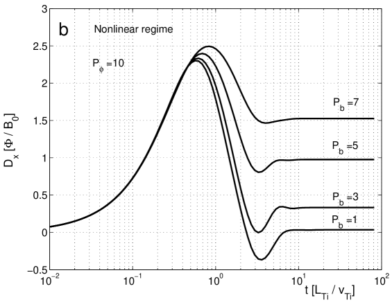
Figure 1: Time dependent diffusion coefficient for $\tau_{c}\rightarrow\infty,$ $\lambda_{z}\rightarrow\infty,$ and the values of the RMP amplitude that label the curves (a) in the quasilinear regime with $P_{\phi}=1$, and (b) in the nonlinear regime with $P_{\phi}=10$. $\overline{V}_{d}=1$.

Typical examples of the time dependent diffusion coefficient in the presence of RMPs are shown in Figure 1.a. for the quasilinear conditions ($P_{\phi}=1),$ and in Figure 1.b. for the nonlinear case $(P_{\phi}=10).$ One can see that the RMPs determine the saturation of $D_{x}(t)$ at finite values in all cases.

In the absence of the RMPs, the transport is subdiffusive in both quasilinear and nonlinear regimes. The RMPs make the transport diffusive, which means that they provide a decorrelation mechanism. Therefore, the RMPs enhance the stochastic aspects of the trajectories by destroying the quasi-coherent structures. The increase of the transport coefficient is expected in such conditions.

Since the RMPs provide a decorrelation mechanism, their effects on the asymptotic diffusion coefficients should be understood from the analysis of the competition with the other decorrelation mechanisms.

The RMPs could produce decorrelation by the average velocity (39) or by trajectory spreading (37) since both processes are induced by RMPs. The examination of the EC of the effective potential (44) shows that the average displacement $\left\langle x_{b}(t)\right\rangle$ does not modify the EC, but it only determines a shift of the EC. The RMP average velocity does not contribute to the decorrelation. It actually determines a radial drift of the stochastic potential.

The asymptotic diffusion coefficient $\chi_{x}$ is shown in Figure 2 as a function of the normalized amplitude of the RMPs for the quasilinear regime (continuous line) and for the nonlinear regime (dashed line). One can see that the transport both regimes is not affected at small $P_{b}$, and that there is a smooth transition to a rather strong degradation of the confinement. At larger amplitudes, the tendency is reversed and the diffusion coefficient decreases.

Similar dependences on $P_{b}$ are found in the quasilinear and nonlinear regimes. There are however some important differences. The maximum diffusion $\chi_{x}^{\max}$ and the corresponding RMP amplitude $P_{b}^{\max}$ do not depend on turbulence amplitude $P_{\phi}$ in the nonlinear transport while they are increasing functions of $P_{\phi}$ in the quasilinear regime. The increase of $\chi_{x}$ in the quasilinear regime is much smaller than in the nonlinear regime. The maximum amplification factor is four times larger in the nonlinear regime in the examples shown in Figure 2. Also the maximum corresponds to smaller amplitudes of the RMPs in the quasilinear case.

The nonlinear dependence of $\chi_{x}$ on $P_{b}$ seen in Figure 2 is explained by the decorrelation effect produced by the RMPs. The decorrelation time $\tau_{b}$ is determined as solution of

$$\left\langle x_{b}^{2}(\tau_{b})\right\rangle=\overline{\lambda}_{x}^{2},$$ (56)

where $\left\langle x_{b}^{2}(t)\right\rangle$ is given by Eq. (37). Since $\left\langle x_{b}^{2}(t)\right\rangle\sim P_{b}^{2},$ $\tau_{b}$ decreases when $P_{b}$ increases. The decorrelation of the turbulence is determined by the parallel motion, and the corresponding decorrelation time $\tau_{z}$ is the solution of

$$\left\langle z^{2}(\tau_{z})\right\rangle=\overline{\lambda}_{z}^{2}.$$ (57)

One obtains $\tau_{z}=$ $\overline{\lambda}_{z}$ if $\tau_{z}\ll 1/P_{c}$ (or $\overline{\lambda}_{z}P_{c}\ll 1),$ and $\tau_{z}=$ $\overline{\lambda}_{z}^{2}P_{c}$ if $\tau_{z}\gg 1/P_{c}$ (or $\overline{\lambda}_{z}P_{c}\gg 1).$ At small $P_{b},$ $\tau_{b}$ is large ($\tau_{z}\ll\tau_{b}),$ which means that the decorrelation is determined by the parallel motion and the RMPs do not influence the diffusion process. As the RMP amplitude increases, $\tau_{b}$  decreases and the RMP decorrelation become dominant. They determine the release of an increasing fraction of trapped trajectories, which contributes to the diffusion and increases $\chi_{x}.$ This tendency is reversed after the release of all trajectories. In these conditions, $\chi_{x}=V_{x}^{2}\tau_{b},$ and it decreases with the increase of $P_{b}.$

Typical values of $P_{b}$ in the present experiments are less than one. In this range, the quasilinear regime is characterized by a stronger influence of the RMPs than the nonlinear transport (Figure 2). The smooth threshold in the dependence of the diffusion coefficient on the amplitude of the RMPs is in agreement with the experiments [7], [4].

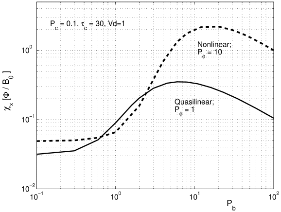
Figure 2: Asymptotic diffusion coefficient as a function of the normalized amplitude of the RMPs for a set of parameters that corresponds to the nonlinear regime.

Figure 3: The average velocity as function of the correlation time for a large domain of the amplitudes of the RMPs, $P_{b}=1,...,50$. The dashed (red) curve is the average velocity in the absence of RMPs.

The gradient of the toroidal magnetic field generates an average velocity (39) of the trajectories $x_{b}(t)$ determined by the RMPs. A similar effect was found in the case of turbulent plasmas [28], [29]. The turbulent pinch velocity is positive in the quasilinear regime corresponding to small $\tau_{c},$ and it becomes negative (directed inward) in the nonlinear regime (large $\tau_{c})$ (see Figure 3, the dashed line).

We determine here the influence of the RMPs on the turbulent pinch velocity. As seen in Figure 3, the effect is complex and it depends on the amplitude of the RMPs, and on the decorrelation time of the turbulence. The RMPs lead to continuous decrease of the quasilinear pinch. In the nonlinear regime, a much more complicated dependence on $P_{b}$ is found. A fast growth of $\left\langle v_{x}\right\rangle$ appears at small $P_{b},$ which reaches positive (outward) values. After a maximum for $P_{b}\simeq 1,$ the pinch decreases and becomes negative. Its minimum decreases and moves toward smaller $\tau_{c}$ as $P_{b}$ increases. The maximum negative velocity is found at $P_{b}\simeq 20$ and $\tau_{c}\simeq 1.$ At very large values of the order $P_{b}>20,$ the absolute value of the minimum $\left\langle v_{x}\right\rangle$ decreases.

The effect of the pinch velocity is determined by the dimensionless parameter $p\equiv L_{T_{i}}\left\langle v_{x}\right\rangle/\chi_{x},$ the peaking factor. It is the estimation of the ratio of the average and the diffusive displacements. The peaking factor for the direct contribution of the RMPs is small $p_{RMP}=L_{T_{i}}/\overline{R}\cong 0.2.$ The turbulent peaking factor decreases due to the RMPs, because the diffusion coefficient increases. However, it can be much larger than $p_{RMP}.$ Values of the order $\gtrsim 1$ can be attained only for $P_{b}\simeq 1$ and for large size plasmas with $a/\rho_{i}\simeq 1000.$ As seen in Figure 3, the pinch is positive at such values, and it contributes to confinement degradation.

5 Conclusions and discussions

The direct effects of the RMPs on turbulent transport were analyzed. The diffusion coefficient and the pinch velocity were determined as functions of the turbulence parameters and of the RMPs amplitude $P_{b}$ in the framework of the test particle approach using a semi-analytical method, the DTM. We underline that the effects of the RMPs on turbulence are neglected in this evaluations. The influence of the stochastic magnetic field generated by the RMPs are rather complex, especially in the nonlinear regime that corresponds to trajectory trapping or eddying. One of the effects, which is well demonstrated and understood, is the attenuation of the modes determined by the increased diffusion, which leads to the decrease of $\Phi$. But other processes could have opposite effects on turbulence amplitude or they can even generate a different type of turbulence.

We have shown that the effects observed in experiments (increased turbulent transport and generation of outward pinch) occur even when the turbulence is not modified by the RMPs. A direct influence of the RMPs on transport is produced through a decorrelation mechanism.

The dependence of the diffusion coefficient on the amplitude of the RMPs is nonlinear (Figure 2). A smooth threshold exists at small $P_{b}.$ It is determined by the condition that the characteristic time of the RMP decorrelation that is a decreasing function on $P_{b}$ should be smaller than the parallel decorrelation time. At larger $P_{b},$ the increase of the transport coefficients appear in both quasilinear and nonlinear regimes, with stronger effect in the first case. The increase is limited, and, after a maximum, the transport enters into a decaying regime. The maximum is very large in the nonlinear regime ($40$ times larger than in the absence of the RMPs) and it appears at very large amplitudes ($P_{b}\simeq 20).$ In the quasilinear regime, the the maximum is much smaller (by a factor five in the example in Figure 2) and the RMP amplitude at the maximum is of the order $P_{b}^{\max}\simeq 5.$ Both $P_{b}^{\max}$ and $\chi_{x}^{\max}$ decrease as the turbulence amplitude decreases.

These results are in agreement with the experiments, which correspond to values of the RMP amplitude $P_{b}\lesssim 1$ and lead to increases of the diffusion coefficients of the order $50-100\%.$ These values of $P_{b}$ are close to the smooth threshold where similar variation of $\chi_{x}$ can be seen in Figure 2. According to our model, the results of the present experiments cannot be extrapolated to ITER conditions. A much faster increase with $P_{b}$ occurs at larger $P_{b}.$ We have found a large difference between the nonlinear and the quasilinear transport at $P_{b}\simeq 10,$ which corresponds to the RMPs of the the order of $1\%$ in ITER plasmas. The confirmation of the transition of the ITG transport from the Bohm to the gyro-Bohm regime and demonstration that the gyro-Bohm transport is of quasilinear type are very important in this context.

We have also analyzed the effect of the RMPs on the turbulent pinch velocity. We have shown that at large correlation times, the negative (inward) drift (dashed curve in Figure 3) is reduced by the RMPs, then they generate a positive (outward) drift that is maximum for $P_{b}\simeq 1.$ At larger $P_{b}$ the average velocity decreases and becomes again negative, which correspond to the prediction of an inward pinch in ITER conditions, but with small values of the peaking.

Acknowledgements

This work was supported by the Romanian Ministry of National Education under the contract 1EU-10 in the Programme of Complementary Research in Fusion. The views presented here do not necessarily represent those of the European Commission.

References

- [1] Evans T. E. 2015 Plasma Phys. Control. Fusion 57 123001
- [2] Kirk A. et al 2013 Plasma Phys. Control. Fusion 55 124003
- [3] Wade M.R. et al 2015 Nucl. Fusion 55 023002
- [4] McKee G.R. et al 2013 Nucl. Fusion 53 113011
- [5] Mordijck S. et al 2010 Nucl. Fusion 50 034006
- [6] Conway G. D. et al 2015 Plasma Phys. Control. Fusion 57 014035
- [7] Mordijck S. et al 2015 Plasma Phys. Control. Fusion 58 014003
- [8] Rea C. et al 2015 Nucl. Fusion 55 113021
- [9] Jakubowski M.W. et al 2013 Nucl. Fusion 53 113012
- [10] Monnier A. et al 2014 Nucl. Fusion 54 064018
- [11] Wingen A., Spatschek K.H. 2010 Nucl. Fusion 50, 034009
- [12] Leconte M. et al 2014 Nucl. Fusion 54 013004
- [13] Vlad M., Spineanu F. 2013 Phys. Plasmas 20 122304
- [14] Vlad M., Spineanu F. 2015 Physics of Plasmas 22 112305
- [15] Vlad M. et al 1998 Phys. Rev. E 58, 7359
- [16] Taylor G. I. 1921 Proc. London Math. Soc. 20 196
- [17] R. Balescu, Aspects of Anomalous Transport in Plasmas, Institute of Physics (IoP), Bristol and Philadelphia, 2005.
- [18] Idomura Y., Nakata M. 2014 Phys. Plasmas 21 020706
- [19] Sarazin Y. et al 2010 Nuclear Fusion 50 054004
- [20] Watanabe T. H. et al 2015 Phys. Plasmas 22 022507
- [21] Xiao Y., Lin Z. 2009 Phys. Rev. Lett. 103, 085004
- [22] Abdullaev S. S. (2012) Nucl. Fusion 52 054002
- [23] Rechester A. B., Rosenbluth M. N. 1978 Phys. Rev. Lett. 40 38
- [24] Vlad M., Spineanu F. 2015 Astrophys. J. (2015) in print
- [25] Vlad M., Spineanu F. 2004 Phys. Rev. E 70, 056304
- [26] Vlad M., Spineanu F. 2015 Romanian Reports in Physics 67 573
- [27] Vlad M. 2013 Phys. Rev. E 87 053105
- [28] Vlad M. et al 2006 Phys. Rev. Lett. 96 085001
- [29] Vlad M. et al 2008 Phys. Plasmas 15 032306