Multilevel Hybrid Split-Step Implicit Tau-Leap

Abstract

In biochemically reactive systems with small copy numbers of one or more reactant molecules, the dynamics is dominated by stochastic effects. To approximate those systems, discrete state-space and stochastic simulation approaches have been shown to be more relevant than continuous state-space and deterministic ones. In systems characterized by having simultaneously fast and slow timescales, existing discrete space-state stochastic path simulation methods, such as the stochastic simulation algorithm (SSA) and the explicit tau-leap (explicit-TL ) method, can be very slow. Implicit approximations have been developed to improve numerical stability and provide efficient simulation algorithms for those systems. Here, we propose an efficient Multilevel Monte Carlo (MLMC) method in the spirit of the work by Anderson and Higham (2012). This method uses split-step implicit tau-leap (SSI-TL ) at levels where the explicit-TL method is not applicable due to numerical stability issues. We present numerical examples that illustrate the performance of the proposed method.

1 Introduction

In his work, we extend the split-step backward-Euler method introduced in [28] to numerically solve stochastic differential equations (SDEs) driven by Brownian motion to the setting of SDEs driven by Poisson random measures [13, 33].

We focus on a particular class of continuous-time Markov chains named stochastic reaction networks (SRNs) (see Section 2.1 for a short introduction). SRNs are employed to describe the time evolution of biochemical reactions, epidemic processes [11, 12], and transcription and translation in genomics and virus kinetics [27, 42], among other important applications. Let $\mathbf{X}$ be an SRN taking values in $\mathbb{Z}_{+}^{d}$ and defined in the time-interval $[0,T]$, where $T>0$ is a user-selected final time. We aim to provide accurate estimations of the expected value, $\mathrm{E}\left[g(\mathbf{X}(T))\right]$, where $g:\mathbb{R}^{d}\to\mathbb{R}$ is a given smooth scalar observable of $\mathbf{X}$.

Many methods have been developed to simulate exact sample paths of SRNs; for instance, the stochastic simulation algorithm (SSA) was introduced by Gillespie in [24] and the modified next reaction method (MNRM) was proposed by Anderson in [7]. It is well known that pathwise exact realizations of SRNs may be computationally very costly when some reaction channels have high reaction rates. To overcome this issue, Gillespie [25] and Aparicio and Solari [30] independently proposed the explicit tau-leap (TL) method (see Section 2.2) to simulate approximate paths of $\mathbf{X}$ by evolving the process with fixed time steps, keeping the reaction rates fixed within each time step.

In this work, we address the problem of producing approximate-path simulations of SRNs for cases in which the set of reaction channels can be clearly classified into two subsets: fast and slow reaction channels (in the literature, this type of problem is called a stiff problem [3, 40]). In this context, the explicit-TL method is hardly adequate because the time step required to maintain the numerical stability can be very small [17, 41] and, as a consequence, simulating explicit-TL paths of process $\mathbf{X}$ may become computationally expensive. For this purpose, different implicit schemes have been suggested, in particular, the drift-implicit tau-leap [40], which uses an implicit discretization for the drift, together with an explicit discretization of the Poissonian noise. Our split-step implicit tau-leap (SSI-TL ), method naturally produces values in the lattice, $\mathbb{Z}_{+}^{d}$. Hence, there is no need for an additional rounding step as in [40] (see Section 2.3).

Other simulation schemes have been proposed to deal with situations with well-separated fast and slow timescales. Cao and Petzold [16] proposed a trapezoidal implicit tau-leap formula that is similar to the trapezoidal rule for solving ordinary differential equations (ODEs). The trapezoidal implicit tau-leap scheme is numerically stable and does not possess the damping effect present in the drift-implicit tau-leap (Section 3 in [17] gives details on the damping effect). In [16], the authors focus on the stability properties of a trapezoidal implicit tau-leap scheme. They provide a posteriori comparisons of moments of order one and two with the SSA, the explicit-TL and the drift-implicit tau-leap methods. To the best of our knowledge, no multilevel version of the trapezoidal tau-leap has been proposed. In [5], Ahn et al. developed fully implicit tau-leap schemes that implicitly treat both the drift and the noise of the Poisson variables. The construction of fully implicit tau-leap schemes is based on adapting weakly convergent discretizations of stochastic differential equations [31] to stochastic chemical kinetic systems. Constructing a multilevel version of the fully implicit tau-leap is still under investigation since it may involve a more complicated way of coupling two consecutive paths than does the SSI-TL presented here. In the same context, Rathinam et al. [39] developed an explicit method that addresses stiffness in small number systems. The reversible-equivalent-monomolecular tau method (REMM-$\tau$) consists of decomposing the system into reversible pairs of reactions and approximating bimolecular reversible pairs by suitable monomolecular reversible pairs. Updating the state of the system involves the use of both binomial and Poisson random variables. The authors in [39] showed that REMM-$\tau$ performs better than the drift-implicit [40] and the trapezoidal implicit [17, 16] tau-leap methods for small number stiff problems, since it avoids the need for an additional rounding step required in the latter methods. Howerver, REMM-$\tau$ does not have a natural multilevel Monte Carlo (MLMC) version (see Section 3.2). Another type of explicit method that addresses stiffness was developed in [3] by Abdulle et al. They proposed $\tau$-ROCK (Orthogonal Runge-Kutta Chebyshev) as an extension of the multi-stage S-ROCK methods [1, 2, 4] for discrete stochastic processes and they derived schemes for processes with discrete Poisson noise. This method can have comparable stability properties to the implicit method while remaining explicit. The stability properties of $\tau$-ROCK can be controlled by increasing the tuning parameter, which is the stage number. Although the $\tau$-ROCK method has the advantage of avoiding the cost of solving nonlinear problems involved in SSI-TL , another cost is included that is related to the selection procedure for the optimal number of stages to obtain a desired stability domain. In [3], Abdulle et al. did not provide an explicit comparison between $\tau$-ROCK and drift-implicit tau-leap in terms of computational time and error control. Furthermore, to the best of our knowledge, no multilevel version of $\tau$-ROCK has been developed for SRNs. The multilevel estimator proposed here is based on the split-step implicit tau-leap (SSI-TL ) rather than on $\tau$-ROCK for two reasons: the first is that coupling two consecutive paths is simpler in the case of the SSI-TL than in the case of the one based on $\tau$-ROCK, which is currently under investigation; the second is that simulating single paths with SSI-TL is more computationally efficient than with $\tau$-ROCK, especially in the case of large time steps (see Section 4). Finally, we mention the so-called integral tau methods proposed in [44], in which the authors developed two variants of tau-leap methods that are adapted to stiff problems, produce nonnegative and lattice valued solutions, and converge to the implicit Euler solution in the fluid limit. This is achieved in two steps: i) a deterministic implicit step that computes the drift update, and ii) a stochastic step based on the search for a set of feasible reaction counts that adds a linear combination of independent binomial and Poisson random variables. Nevertheless, those methods cannot be naturally extended to the MLMC paradigm.

We mention a few works on error analysis and convergence in implicit tau-leap schemes [41, 38]. In [41], Rathinam et al. showed that both the explicit and the implicit tau-leap methods are first-order convergent in all moments under the assumptions of bounded state space and linear propensity functions. This result was generalized for nonlinear propensity functions in [33] but only specifically for the explicit-TL method. This type of method has $1/2$ order of convergence in a strong sense. Discussions of the two existing scalings for the convergence analysis of tau-leap methods can be found in [9, 29]. More general results for the weak convergence were established in [38] for unbounded systems that possess certain moment growth bounds. Rathinam [41] showed that the main convergence result applies to any tau-leap method provided that it produces integer-valued states and satisfies some condition related to the moments, particularly implicit methods.

Inspired by the work of Anderson and Higham [6, 23], we extend the SSI-TL idea to the multilevel setting by introducing a multilevel hybrid SSI-TL estimator (see Section 3) with the aim of reducing the computational work needed to compute an estimate of $\mathrm{E}\left[g(\mathbf{X}(T))\right]$ within a fixed tolerance, $TOL$, with a given level of confidence, and for a class of systems characterized by having simultaneously fast and slow time scales. Our MLMC strategy couples two SSI-TL paths at the coarser levels of discretization until a certain interface level, $L^{\text{int}}$, where we start coupling paths using the explicit-TL method as indicated in [6]. In that sense, our strategy can be considered to be a hybrid algorithm. This strategy is specially relevant when $TOL$ is small, implying that the finest level of the multilevel SSI-TL , $L^{\text{imp}}$, is in the stability regime of the multilevel explicit-TL . For large values of $TOL$, our MLMC estimator reduces to a multilevel SSI-TL estimator.

As noted above, this extension is relevant to systems with slow and fast timescales (see Section 4 for numerical examples). In such situations, the multilevel estimator given in [6] is not computationally efficient due to the numerical stability constraint. In Section 4, we show that the multilevel SSI-TL method has the same order of computational complexity as the multilevel explicit-TL , which is of ${\mathcal{O}}\left(TOL^{-2}\log(TOL)^{2}\right)$ [10], but with a smaller multiplicative constant. We note that here our goal is to provide an estimate of $\mathrm{E}\left[g(\mathbf{X}(T))\right]$ in the probability sense and not in the mean-square sense as in [6].

Recently, adaptive multilevel estimators were proposed to improve the performance of non-adaptive estimators [6] to simulate SRNs with markedly different timescales. In [35], Moraes et al. presented an adaptive MLMC method that uses a low-cost, reaction-splitting heuristic to adaptively classify the set of reaction channels into two subsets, fast and slow, in terms of level of activity. Based on their adaptive reaction-splitting technique and using a hierarchy of non-nested time meshes, they simulate the increments associated with high activity channels (fast reactions) using the explicit-TL method while those associated with low activity channels (slow reactions) are simulated using an exact method. Lester et al. [32] proposed an adaptive MLMC method strongly influenced by [6] that uses a time-stepping strategy based on the concept of the leap condition introduced in [15]. The idea of adaptivity provides possibilities for future research directions, for instance developing efficient, adaptive, hybrid multilevel estimators that would allow us to switch between using SSI-TL , explicit-TL and exact SSA within the course of a single sample path.

The outline of the remainder of this work is as follows: in Section 2, we introduce the mathematical model of SRNs and give the necessary elements to simulate single-level SSI-TL paths in the context of SRNs. In Section 3, we introduce our multilevel hybrid SSI-TL estimator. First, we review the MLMC method and then we show how to couple SSI-TL paths and also a SSI-TL path with another path simulated by the explicit-TL method. This coupling procedure is the main building block for constructing the new MLMC estimator. This section ends with a presentation of the implementation details of the proposed estimator, which involves the procedure to select the levels and number of simulations per level and the switching rule from coupled SSI-TL to explicit-TL . In Section 4, we present some numerical experiments illustrating the performance of the proposed method. Finally, in Section 5, we offer conclusions and suggest directions for future work.

2 Single-Level SSI-TL Path-Simulation of Stochastic Reaction Networks

In this section, we briefly introduce the definition of stochastic reaction networks (SRNs). Then, we review the explicit-TL method. Finally, we present the SSI-TL scheme, which can be seen as an extension of the split-step backward-Euler method [28] to the context of SRNs.

2.1 Stochastic Reaction Networks

We are interested in the time evolution of a homogeneously mixed chemical reacting system described by the Markovian pure jump process, $\mathbf{X}:[0,T]\times\Omega\to\mathbb{Z}_{+}^{d}$, where ($\Omega$, $\mathcal{F}$, $P$) is a probability space. In this framework, we assume that $d$ different species interact through $J$ reaction channels. The $i$-th component, $X_{i}(t)$, describes the abundance of the $i$-th species present in the chemical system at time $t$. Hereafter, $\mathbf{v}^{T}$ denotes the transpose of the vector $\mathbf{v}$. The aim of this work is to study the time evolution of the state vector,

$$\mathbf{X}(t)=(X_{1}(t),\ldots,X_{d}(t))^{T}\in\mathbb{Z}_{+}^{d}.$$

Each reaction channel, $\mathcal{R}_{j}$, is a pair $(a_{j},\boldsymbol{\nu}_{j})$, defined by its propensity function, $a_{j}:\mathbb{R}^{d}\rightarrow\mathbb{R}_{+}$, and its state change vector, $\boldsymbol{\nu}_{j}=(\nu_{j}^{1},\nu_{j}^{2},...,\nu_{j}^{d})^{T}$, satisfying

(1) $$\mathrm{P}\left(\mathbf{X}(t+\Delta t)=\mathbf{x}+\boldsymbol{\nu}_{j}\bigm{|}\mathbf{X}(t)=\mathbf{x}\right)=a_{j}(\mathbf{x})\Delta t+{o}\left(\Delta t\right),\>j=1,2,...,J.$$

Formula (1) states that the probability of observing a jump in the process, $\mathbf{X}$, from state $\mathbf{x}$ to state $\mathbf{x}+\boldsymbol{\nu}_{j}$, a consequence of the firing of the j-th reaction, $\mathcal{R}_{j}$, during a small time interval, $(t,t+\Delta t]$, is proportional to the length of the time interval, $\Delta t$, with $a_{j}(\mathbf{x})$ as the constant of proportionality.

We set $a_{j}(\mathbf{x}){=}0$ for those $\mathbf{x}$ such that $\mathbf{x}{+}\boldsymbol{\nu}_{j}\notin\mbox{$\mathbb{Z}_{+}^{d}$}$ (the non-negativity assumption: the system can never produce negative population values).

As a consequence of relation (1), process $\mathbf{X}$ is a continuous-time, discrete-space Markov chain that can be characterized by the random time change representation of Kurtz [22]:

(2) $$\mathbf{X}(t)=\mathbf{x}_{0}+\sum_{j=1}^{J}Y_{j}\left(\int_{0}^{t}a_{j}(\mathbf{X}(s))\,\mathrm{d}s\right)\boldsymbol{\nu}_{j},$$

where $Y_{j}:\mathbb{R}_{+}{\times}\Omega\to\mathbb{Z}_{+}$ are independent unit-rate Poisson processes. Conditions on the set of reaction channels can be imposed to ensure uniqueness [11] and to avoid explosions in finite time [37, 26, 21]

2.2 The Explicit-TL Approximation

In this section, we briefly review the explicit-TL approximation of the process, $\mathbf{X}$.

The tau-leap is a pathwise-approximate method independently introduced in [25] and [30] to overcome the computational drawback of exact methods, i.e., when many reactions fire during a short time interval. It can be derived from the random time change representation of Kurtz (2) by approximating the integral $\int_{t_{i}}^{t_{i+1}}a_{j}(\mathbf{X}(s))\mathrm{d}s$ by $a_{j}(\mathbf{X}(t_{i}))\,(t_{i+1}-t_{i})$, i.e., using the forward-Euler method with a time mesh $\{t_{0}=0,t_{1},...,t_{N}=T\}$. In this way, the explicit-TL approximation of $\mathbf{X}$ should satisfy for $k\in\{1,2,\ldots,N\}$:

$$\mathbf{Z}^{exp}(t_{k})=\mathbf{x}_{0}+\sum_{j=1}^{J}Y_{j}\left(\sum_{i=0}^{k-1}a_{j}(\mathbf{Z}^{exp}(t_{i}))(t_{i+1}-t_{i})\right)\boldsymbol{\nu}_{j}.$$

By considering a uniform time mesh of size $\tau$, we can simulate a path of $\mathbf{Z}^{exp}$ as follows. Let $\mathbf{Z}^{exp}(t_{0}):=\mathbf{x}_{0}$ and define

(3) $$\mathbf{Z}^{exp}(t_{k}):=\mathbf{z}+\sum_{j=1}^{J}\mathcal{P}_{j}(a_{j}(\mathbf{z})\tau)\boldsymbol{\nu}_{j},$$

iteratively, where $\mathbf{z}=\mathbf{Z}^{exp}(t_{k-1})$ and $\mathcal{P}_{j}(r_{j})$ are independent Poisson random variables with respective rates, $r_{j}$. Notice that the explicit-TL path, $\mathbf{Z}^{exp}$, is defined only at the points of the time mesh, but it can be naturally extended to $[0,T]$ as a piecewise constant path by defining $\mathbf{Z}^{exp}(t_{k-1}+h):=\mathbf{Z}^{exp}(t_{k-1}),\forall\,\,0<h<\tau$.

2.2.1 Numerical Stability of the Explicit-TL Method

The numerical stability of the explicit-TL method is treated in [41] for the case of linear propensities, i.e., $\>a_{j}(\mathbf{X})=\mathbf{c}^{T}_{j}\mathbf{X}$, where $\mathbf{c}_{j}\in\mathbb{R}^{d}$. In this particular case, taking expectations of relation (3) conditional on $\mathbf{z}$ results in

(4) $$\mathrm{E}\left[\mathbf{Z}^{exp}(t_{k})\mid\mathbf{z}\right]=(1+\tau A)\mathbf{z},$$

where the $d\times d$ matrix $\mathbf{A}$ is given by $\mathbf{A}=\sum\limits_{j=1}^{J}\boldsymbol{\nu}_{j}\mathbf{c}_{j}^{T}$.

Taking the expectation of (4), we obtain

(5) $$\mathrm{E}\left[\mathbf{Z}^{exp}(t_{k})\right]=(1+\tau A)\mathrm{E}\left[\mathbf{z}\right],$$

which yields

(6) $$\mathrm{E}\left[\mathbf{Z}^{exp}(t+N\tau)\right]=(1+\tau A)^{N}\mathrm{E}\left[\mathbf{Z}^{exp}(t)\right].$$

Then, from (5), the expectation of the explicit-TL method is asymptotically stable if $\tau$ satisfies

$$\mid 1+\tau\lambda_{i}(\mathbf{A})\mid<1,\>\>i=1,\dots,d,$$

where $\{\lambda_{i}\}_{i=1}^{d}$ are the eigenvalues of the matrix $\mathbf{A}$.

In the general case, the numerical stability limit of the explicit-TL method can be computed by a linearized stability analysis of the forward-Euler method applied to the corresponding deterministic ODE model [40]. In the case of systems having simultaneously fast and slow timescales, this stability limit can be very small, implying an expensive computational cost for simulation. To overcome this issue, the drift-implicit tau-leap idea [40] has been proposed. We should note that using implicit methods is only relevant in the case of negative eigenvalues. In fact, having a positive eigenvalue implies a rapid change in the solution, which requires the use of a small time step. Using explicit methods is more appropriate under such conditions.

2.3 The SSI-TL Approximation

In this section, we define $\mathbf{Z}^{imp}$, the SSI-TL approximation of the process, $\mathbf{X}$.

The explicit-TL scheme (3), where $\mathbf{z}=\mathbf{Z}^{exp}(t)$, can be rewritten as follows:

$$\mathbf{Z}^{exp}(t+\tau) =\mathbf{z}+\sum_{j=1}^{J}\mathcal{P}_{j}\left(a_{j}(\mathbf{z})\tau\right)\boldsymbol{\nu}_{j}$$

$$=\mathbf{z}+\sum_{j=1}^{J}\left(\mathcal{P}_{j}\left(a_{j}(\mathbf{z})\tau\right)-a_{j}(\mathbf{z})\tau+a_{j}(\mathbf{z})\tau\right)\boldsymbol{\nu}_{j}$$

(7) $$=\mathbf{z}+\sum_{j=1}^{J}a_{j}(\mathbf{z})\tau\boldsymbol{\nu}_{j}+\sum_{j=1}^{J}\left(\mathcal{P}_{j}\left(a_{j}(\mathbf{z})\tau\right)-a_{j}(\mathbf{z})\tau\right)\boldsymbol{\nu}_{j}.$$

Let us denote the second and third quantities on the right-hand side of (2.3) by the drift and the zero-mean noise, respectively. The idea of the SSI-TL method is to take only the drift part as implicit while the noise part is left explicit. Let us define $\mathbf{z}=\mathbf{Z}^{imp}(t)$ and define $\mathbf{Z}^{imp}(t+\tau)$ through the following two steps:

(8) $$\mathbf{y} =\mathbf{z}+\sum_{j=1}^{J}a_{j}\left(\mathbf{y}\right)\tau\boldsymbol{\nu}_{j}\text{ (Drift-Implicit step)}$$

$$\mathbf{Z}^{imp}(t+\tau) =\mathbf{y}+\sum_{j=1}^{J}\left(\mathcal{P}_{j}(a_{j}(\mathbf{y})\tau)-a_{j}(\mathbf{y})\tau\right)\boldsymbol{\nu}_{j}$$

$$=\mathbf{z}+\sum_{j=1}^{J}\mathcal{P}_{j}(a_{j}(\mathbf{y})\tau)\boldsymbol{\nu}_{j}\text{ (Tau-leap step)}.$$

Algorithm 1 Algorithm of the SSI-TL method

.

1:  Fix $\tau>0$. Set $\mathbf{Z}(0)=\mathbf{x}_{0}$, $t_{0}=0$, $n=0$ and repeat the following until $t_{n}\geq T$

2:  Set $t_{n+1}=t_{n}+\tau$. If $t_{n+1}\geq T$, set $t_{n+1}=T$ and $\tau=T-t_{n}$

3:  Implicit step: $\mathbf{Y}=\mathbf{Z}(t_{n})+\sum\limits_{j=1}^{J}a_{j}(\mathbf{Y})\tau\boldsymbol{\nu}_{j}$

4:  Explicit step: $\mathbf{Z}(t_{n+1})=\mathbf{Z}(t_{n})+\sum\limits_{j=1}^{J}\left(\text{Poisson}(a_{j}(\mathbf{Y})\tau)\right)\boldsymbol{\nu}_{j}$

5:  Set $n\leftarrow n+1$

Algorithm 1 implements (8).

Notice that the SSI-TL method naturally produces values of $Z^{\text{imp}}$ in the lattice, $\mathbb{Z}_{+}^{d}$, without the need for a final rounding step as in the drift-implicit method [40], which goes as follows: first compute an intermediate state according to relation (9):

(9) $$\mathbf{Z}^{{}^{\prime}} =\mathbf{z}+\sum_{j=1}^{J}a_{j}(\mathbf{Z}^{{}^{\prime}})\>\tau\>\boldsymbol{\nu}_{j}+\sum_{j=1}^{J}\left(\mathcal{P}_{j}\left(a_{j}(\mathbf{z})\tau\right)-a_{j}(\mathbf{z})\tau\right)\boldsymbol{\nu}_{j}.$$

Then approximate the actual number of firings, $K_{j}(\mathbf{z},\tau)$, of reaction channel $R_{j}$ in the time interval $(t,t+\tau]$ by the integer-valued random variable, $\widetilde{K}_{j}(\mathbf{z},\tau)$, defined by

(10) $$\widetilde{K}_{j}(\mathbf{z},\tau) =\left[a_{j}(\mathbf{Z}^{{}^{\prime}})\tau+\mathcal{P}_{j}\left(a_{j}(\mathbf{z})\tau\right)-a_{j}(\mathbf{z})\tau\right],$$

where $[x]$ denotes the nearest nonnegative integer to $x$. Finally, update the state at time $t+\tau$ such that $\mathbf{Z}(t+\tau)=\mathbf{z}+\sum_{j=1}^{J}\widetilde{K}_{j}(\mathbf{z},\tau)\boldsymbol{\nu}_{j}.$ This rounding procedure in relation (10) introduces an error when simulating the path.

3 Multilevel Hybrid SSI-TL 

The goal of this section is to define our multilevel hybrid SSI-TL estimator. First, we quickly review the MLMC method as proposed by Giles [23]. Then, we show how to couple two SSI-TL paths associated with two nested time meshes. This coupling is the main building block for constructing our novel multilevel hybrid SSI-TL estimator. Finally, we present the switching rule that we use to select the time mesh in which we move from the SSI-TL method to the explicit-TL one. For simplicity, in this section, we consider only uniform time meshes in the interval $[0,T]$.

3.1 The Multilevel Monte Carlo (MLMC) Method

Let $\mathbf{X}$ be a stochastic process and $g:\mathbb{R}^{d}\rightarrow\mathbb{R}$ a smooth scalar observable. Let us assume that we want to approximate $\mathrm{E}\left[g(\mathbf{X}(T))\right]$, but instead of sampling directly from $\mathbf{X}(T)$, we sample from $\mathbf{Z}_{h}(T)$, which are random variables generated by an approximate method with step size $h$. Let us assume also that the variates $\mathbf{Z}_{h}(T)$ are generated with an algorithm with weak order, ${\mathcal{O}}\left(h\right)$, i.e., $\mathrm{E}\left[g(\mathbf{X}(T))-g(\mathbf{Z}_{h}(T))\right]={\mathcal{O}}\left(h\right)$.

Let $\mu_{N}$ be the standard Monte Carlo estimator of $\mathrm{E}\left[g(\mathbf{Z}_{h}(T))\right]$ defined by

(11) $$\mu_{N}:=\frac{1}{N}\sum_{n=1}^{N}f(\mathbf{Z}_{h,[n]}(T)),$$

where $\mathbf{Z}_{h,[n]}(T)$ are independent and distributed as $\mathbf{Z}_{h}(T)$.

Consider now the following decomposition of the global error:

(12) $$\mathrm{E}\left[g(\mathbf{X}(T))\right]-\mu_{N}=\left(\mathrm{E}\left[g(\mathbf{X}(T))-g(\mathbf{Z}_{h}(T))\right]\right)+\left(\mathrm{E}\left[g(\mathbf{Z}_{h}(T))\right]-\mu_{N}\right).$$

To have the desired accuracy, $TOL$, it is sufficient to take $h={\mathcal{O}}\left(TOL\right)$ so that the first term on the right is ${\mathcal{O}}\left(TOL\right)$ and, by the Central Limit Theorem, impose $N={\mathcal{O}}\left(TOL^{-2}\right)$ so that the statistical error given by the second term on the right is ${\mathcal{O}}\left(TOL\right)$ [19]. As a consequence, the expected total computational work is ${\mathcal{O}}\left(TOL^{-3}\right)$.

The MLMC estimator, introduced by Giles [23] allows us to reduce the total computational work from ${\mathcal{O}}\left(TOL^{-3}\right)$ to ${\mathcal{O}}\left(TOL^{-2}\log(TOL)^{2}\right)$. The basic idea of MLMC is to generate, and couple in an intelligent manner, paths with different step sizes, which results in

• Stochastically coordinated sequences of paths having different step sizes, where the paths with large step sizes are computationally less expensive than those with very small step sizes.

• A small variance of the difference between two coupled paths with fine step sizes, implying significantly fewer samples in the estimation.

We can construct the MLMC estimator as follows: consider a hierarchy of nested meshes of the time interval $[0,T]$, indexed by $\ell=0,1,\dots,L$. We denote by $h_{0}$ the step size used at level $\ell=0$. The size of the subsequent time steps for levels $\ell\geq 1$ are given by $h_{\ell}=M^{-\ell}h_{0}$, where $M{>}1$ is a given integer constant. In this work, we take $M=2$. To simplify the notation, hereafter $\mathbf{Z}_{\ell}$ denotes the approximate process generated using a step size of $h_{\ell}$.

Consider now the following telescoping decomposition of $\mathrm{E}\left[g(\mathbf{Z}_{L}(T))\right]$:

(13) $$\mathrm{E}\left[g(\mathbf{Z}_{L}(T))\right]=\mathrm{E}\left[g(\mathbf{Z}_{0}(T))\right]+\sum_{\ell=1}^{L}\mathrm{E}\left[g(\mathbf{Z}_{\ell}(T))-g(\mathbf{Z}_{\ell-1}(T))\right].$$

By defining

(14) $$\begin{cases}\hat{Q}_{0}:=\frac{1}{N_{0}}\sum\limits_{n_{0}=1}^{N_{0}}g(\mathbf{Z}_{0,[n_{0}]}(T))\\ \hat{Q}_{\ell}:=\frac{1}{N_{\ell}}\sum\limits_{n_{\ell}=1}^{N_{\ell}}\left(g(\mathbf{Z}_{\ell,[n_{\ell}]}(T))-g(\mathbf{Z}_{\ell-1,[n_{\ell}]}(T))\right),\\ \end{cases}$$

we arrive at the unbiased MLMC estimator, $\hat{Q}$, of $\mathrm{E}\left[g(\mathbf{Z}_{L}(T))\right]$:

(15) $$\hat{Q}:=\sum\limits_{\ell=0}^{L}\hat{Q}_{\ell}.$$

We note that the key point here is that both $\mathbf{Z}_{\ell,[n_{\ell}]}(T)$ and $\mathbf{Z}_{\ell-1,[n_{\ell}]}(T)$ are sampled using different time discretizations but with the same generated randomness. If we simulate the paths with a method having a strong error of order $1/2$, i.e., $\mathrm{E}\left[\mid\mid\mathbf{Z}_{h}(T)-\mathbf{X}(T)\mid\mid^{2}\right]={\mathcal{O}}\left(h\right)$, and we assume that $g$ is Lipschitz, i.e., $\exists\>c\geq 0\>\>\text{s.t}\>\mid g(\mathbf{X})-g(\mathbf{Y})\mid\leq c\mid\mid\mathbf{X}-\mathbf{Y}\mid\mid$, it is straightforward to see that

$$\mathrm{Var}\left[g(\mathbf{Z}_{\ell}(T))-g(\mathbf{Z}_{\ell-1}(T))\right]={\mathcal{O}}\left(h_{l}\right).$$

Therefore, by setting $N_{\ell}={\mathcal{O}}\left(TOL^{-2}\times L\times h_{\ell}\right)$, we obtain $\mathrm{Var}\left[\hat{Q}\right]={\mathcal{O}}\left(TOL^{2}\right)$ but with a total computational complexity of ${\mathcal{O}}\left(TOL^{-2}\log(TOL)^{2}\right)$, which makes the MLMC estimator better than the standard MC estimator (11) for computational purposes.

3.2 Coupling Two SSI-TL Paths

Algorithm 2, inspired by [6], shows how to couple two explicit-TL paths. Note that $d$ is the number of species and $J$ is the number of reactions.

Algorithm 2 Simulation of two coupled SSI-TL paths.

1:  Fix $h_{\ell}>0$ and set $h_{\ell-1}=2\times h_{\ell}$. Set $\mathbf{Z}_{\ell}(0)=\mathbf{Z}_{\ell-1}(0)=\mathbf{x}_{0}$, $t_{0}=0$, $n=0$.

2:  while $t_{n}<T$ do

3:     Implicit step for the finer level: Solve $\widetilde{\mathbf{Z}}_{\ell}(t_{n})=\mathbf{Z}_{\ell}(t_{n})+\sum\limits_{j=1}^{J}a_{j}(\widetilde{\mathbf{Z}}_{\ell}(t_{n}))h_{\ell}\boldsymbol{\nu}_{j}$

4:     Implicit step for the coarser level:

5:     if $(n\>mod\>2)=0$ then

6:        Solve $\widetilde{\mathbf{Z}}_{\ell-1}(t_{n})=\mathbf{Z}_{\ell-1}(t_{n})+\sum\limits_{j=1}^{J}a_{j}(\widetilde{\mathbf{Z}}_{\ell-1}(t_{n}))h_{\ell-1}\boldsymbol{\nu}_{j}$

7:     end if

8:     for $j{=}1$ to $J$ do

9:        $A_{3(j-1)+1}=a_{j}(\widetilde{\mathbf{Z}}(t_{n}))\wedge a_{j}(\widetilde{\mathbf{Z}}_{\ell-1}(t_{n}))$

10:        $A_{3(j-1)+2}=a_{j}(\widetilde{\mathbf{Z}}(t_{n}))-A_{3(j-1)+1}$

11:        $A_{3(j-1)+3}=a_{j}(\widetilde{\mathbf{Z}}_{\ell-1}(t_{n}))-A_{3(j-1)+1}$

12:        $\Lambda_{3(j-1)+1}=\>\text{Poisson}\>(A_{3(j-1)+1}h_{\ell})$

13:        $\Lambda_{3(j-1)+2}=\>\text{Poisson}\>(A_{3(j-1)+2}h_{\ell})$

14:        $\Lambda_{3(j-1)+3}=\>\text{Poisson}\>(A_{3(j-1)+3}h_{\ell})$

15:     end for

16:     State updating (explicit step)

• Set $\boldsymbol{\Gamma}_{\ell}=\boldsymbol{\nu}\otimes[1\>1\>0]$ and $\boldsymbol{\Gamma}_{\ell-1}=\boldsymbol{\nu}\otimes[1\>0\>1]$ ($A\otimes B$ refers to the Kronecker product of the matrices $A$ and $B$, therefore $\boldsymbol{\Gamma}_{\ell}$ and $\boldsymbol{\Gamma}_{\ell-1}$ are $d\times 3J$ matrices. Observe that $A$ and $\Lambda$ are of size $3J\times 1$.

• Update $\mathbf{Z}_{\ell}(t_{n+1})=\mathbf{Z}_{\ell}(t_{n})+h_{\ell}\boldsymbol{\Gamma}_{\ell}\Lambda$

• Update $\mathbf{Z}_{\ell-1}(t_{n+1})=\mathbf{Z}_{\ell-1}(t_{n})+h_{\ell}\boldsymbol{\Gamma}_{\ell-1}\Lambda$

17:     $t_{n+1}=t_{n}+h_{\ell}$

18:     $n\leftarrow n+1$,

19:  end while

We define our multilevel hybrid SSI-TL estimator in the next section based on Algorithm 2.

Remark 3.1.

For solving the implicit steps in Algorithm 2, we use the classic Newton method. As an initial guess, we select $\mathbf{X}(0)$. Regarding the number of iterations, we ideally would like to compute an approximate solution, $\mathbf{y^{*}}$, of $\mathbf{y}$ such that the distribution of $\text{Poisson}(a_{j}(\mathbf{y^{*}})\,h)$ is close to the distribution of $\text{Poisson}(a_{j}(\mathbf{y})\,h)$ for all $j\in\{1,2,\ldots,J\}$. In practice, we usually check that the difference between two consecutive iterations, $h\,\max_{j}\left\|\nu_{j}\right\|_{\infty}\,\left|a_{j}(\mathbf{y_{k-1}^{*}})-a_{j}(\mathbf{y_{k}^{*}})\right|$, is below a certain tolerance.

Remark 3.2.

It is well known that tau-leap methods can produce negative population numbers. Methods for avoiding negative population numbers can roughly be divided into three classes: i) the pre-leap check technique [14, 15, 34]; ii) the post-leap check technique [8]; and iii) the modification of the Poisson distributed increments with bounded increments from binomial or multinomial distributions [43]. The pre-leap check technique computes the largest possible time step satisfying some leap criterion. It is often based on controlling the relative change in the propensity function before taking the step. The post-leap check procedure is applied when a step results in a negative population value. In this case, it retakes a shorter step, conditioned on already sampled data from the failed step, to avoid sampling bias. Finally, the third technique consists of projecting negative values of species numbers to zero at each step and continues the path simulation until $T$. In the future, we intend to investigate these techniques in the context of the SSI-TL method.

3.3 Definition of the Multilevel Hybrid SSI-TL Estimator

Our hybrid MLMC estimator uses the multilevel SSI-TL method only at the coarser levels and then, starting from a certain interface level, $L^{\text{int}}$, it switches to the multilevel explicit-TL method as given in [6]. This strategy is specially relevant when $TOL$ is small, implying that the finest level of the multilevel SSI-TL , $L^{\text{imp}}$, is in the stability regime of the multilevel explicit-TL . On the contrary, for sufficiently large values of the tolerance, $TOL$, our estimator is reduced to a multilevel SSI-TL estimator. For simplicity, let us consider a family of uniform time meshes of $[0,T]$, with size $h_{\ell}=2^{-\ell}T$. Let $L_{c}^{\text{imp}}$ and $L_{c}^{\text{exp}}$ be the coarsest levels in which the SSI-TL and the explicit methods are respectively stable. In the class of problems we are interested in, we have the relation $h_{L_{c}^{\text{exp}}}\ll h_{L_{c}^{\text{imp}}}$, which means that $L_{c}^{\text{imp}}$ is much coarser than $L_{c}^{\text{exp}}$.

Rewriting (15) in our context, we define our multilevel hybrid SSI-TL estimator as

(16) $$\hat{Q}:=\hat{Q}_{L_{c}^{\text{imp}}}+\sum\limits_{\ell=L_{c}^{\text{imp}}+1}^{L^{\text{int}}-1}\hat{Q}_{\ell}+\hat{Q}_{L^{\text{int}}}+\sum\limits_{\ell=L^{\text{int}}+1}^{L}\hat{Q}_{\ell},$$

where

(17) $$\begin{cases}\hat{Q}_{L_{c}^{\text{imp}}}:=\frac{1}{N_{i,L_{c}^{\text{imp}}}}\sum\limits_{n=1}^{N_{i,L_{c}^{\text{imp}}}}g(\mathbf{Z}^{imp}_{L_{c}^{\text{imp}},[n]}(T))\\ \hat{Q}_{\ell}:=\frac{1}{N_{ii,\ell}}\sum\limits_{n_{\ell}=1}^{N_{ii,\ell}}\left(g(\mathbf{Z}^{imp}_{\ell,[n_{\ell}]}(T))-g(\mathbf{Z}^{imp}_{\ell-1,[n_{\ell}]}(T))\right),\>\>L_{c}^{\text{imp}}+1\leq\ell\leq L^{\text{int}}-1\\ \hat{Q}_{L^{\text{int}}}:=\frac{1}{N_{ie,L^{\text{int}}}}\sum\limits_{n=1}^{N_{ie,L^{\text{int}}}}\left(g(\mathbf{Z}^{exp}_{L^{\text{int}},[n]}(T))-g(\mathbf{Z}^{imp}_{L^{\text{int}}-1,[n]}(T))\right)\\ \hat{Q}_{\ell}:=\frac{1}{N_{ee,\ell}}\sum\limits_{n_{\ell}=1}^{N_{ee,\ell}}\left(g(\mathbf{Z}^{exp}_{\ell,[n_{\ell}]}(T))-g(\mathbf{Z}^{exp}_{\ell-1,[n_{\ell}]}(T))\right),\>\>L^{\text{int}}+1\leq\ell\leq L.\\ \end{cases}$$

Remark 3.3.

According to (17), computing our MLMC tau-leap estimator (16) may require three types of coupling: i) coupling two consecutive SSI-TL paths (see section 3.2), ii) coupling a SSI-TL path with an explicit-TL path; this coupling is made in a similar way as in Algorithm 2 but instead of an implicit step for the finer level, we do an explicit step, and iii) coupling two consecutive explicit-TL paths [6].

From relations (16) and (17), we notice that our MLMC estimator requires the specification of the coarsest discretization level, $L_{c}^{\text{imp}}$, the interface level, $L^{\text{int}}$, the finest level of discretization, $L$, and the number of samples per level defined by $\mathbf{N}:=\{N_{i,L_{c}^{\text{imp}}},\{N_{ii,\ell}\}_{\ell=L_{c}^{\text{imp}}+1}^{L^{\text{int}}-1},N_{ie,L^{\text{int}}},\{N_{ee,\ell}\}_{\ell=L^{\text{int}}+1}^{L}\}$.

3.3.1 On the Selection of the Coarsest Discretization Level

We start by defining the criterion that we use to choose the value of the coarsest discretization level, $L_{c}^{\text{imp}}$. In fact, to ensure the numerical stability of our MLMC estimator, two conditions must be satisfied: the first one ensures the stability of a single path, which is related to the coarsest level of discretization, $L_{c}$, and which can be determined by a linearized stability analysis of the backward-Euler method applied to the deterministic ODE model corresponding to our SRN system [40]. The second one ensures the stability of the variance of the coupled paths of our MLMC estimator and can be expressed by $\mathrm{Var}\left[g(\mathbf{Z}_{L_{c}^{\text{imp}}+1}){-}g(\mathbf{Z}_{L_{c}^{\text{imp}}})\right]\ll\mathrm{Var}\left[g(\mathbf{Z}_{L_{c}^{\text{imp}}})\right]$.

3.3.2 On the Selection of the Finest Discretization Level

The total number of levels, $L$, and the set of the number of samples per level, $\mathbf{N}$, are selected to satisfy the accuracy constraint, $\mathrm{P}\left(\left|\mathrm{E}\left[g(\mathbf{X}(T))\right]-\hat{Q}\right|<TOL\right)>1-\alpha$ (typically we choose $\alpha=0.05$), with near-optimal expected computational work. Here, $TOL$ is a user-selected tolerance.

The total error can be split into bias and statistical error such that

(18) $$\left|\mathrm{E}\left[g(\mathbf{X}(T))\right]-\hat{Q}\right|\leq\underbrace{\left|\mathrm{E}\left[g(\mathbf{X}(T))-\hat{Q}\right]\right|}_{\text{Bias}}+\underbrace{\left|\mathrm{E}\left[\hat{Q}\right]-\hat{Q}\right|}_{\text{Statistical error}}.$$

If we use a splitting parameter, $\theta\in(0,1)$, satisfying

$$TOL=\underbrace{(1-\theta)\,\,TOL}_{\text{Bias tolerance}}+\underbrace{\theta\,\,TOL}_{\text{Statistical error tolerance}},$$

then, using the same idea introduced in [18], the MLMC algorithm should bound the bias and the statistical error as follows:

(19) $$\left|\mathrm{E}\left[g(\mathbf{X}(T))-\hat{Q}\right]\right| \leq(1-\theta)\,\,TOL,$$

(20) $$\left|\mathrm{E}\left[\hat{Q}\right]-\hat{Q}\right| \leq\theta\,\,TOL,$$

where the latter bound should hold with probability $1{-}\alpha$. As stated in [18], relation (20) can be achieved if we impose

(21) $$\mathrm{Var}\left[\hat{Q}\right]\leq\left(\frac{\theta\,\,TOL}{C_{\alpha}}\right)^{2}$$

for some given confidence parameter, $C_{\alpha}$, such that $\Phi(C_{\alpha})=1-{\alpha}/{2}$ ; here, $\Phi$ is the cumulative distribution function of a standard normal random variable (see [18] for details).

In our numerical examples, we choose $\theta=0.5$. An optimal split between bias and statistical errors can be reached by assuming the dependence of $\theta$ on $TOL$ and applying the Continuation Multilevel Monte Carlo (CMLMC) algorithm, introduced in [18]. Investigating the optimal split in this context will be left as future work.

In our problem, the finest discretization level, $L$, is determined by satisfying relation (19) for $\theta=0.5$, implying

(22) $$\left|\text{Bias}(L):=\mathrm{E}\left[g(\mathbf{X}(T))-g(\mathbf{Z}_{L}(T))\right]\right|<\frac{TOL}{2}.$$

In our numerical experiments, we use the following approximation (see [23]):

(23) $$\text{Bias}(L)\approx\mathrm{E}\left[g(\mathbf{Z}_{L}(T))-g(\mathbf{Z}_{L-1}(T))\right].$$

Therefore, to determine the value of $L$, we need to have estimates of the bias for different levels of discretization, $\ell$. In our numerical examples if $L\leq L_{c}^{\text{exp}}$: then we estimate the bias of the difference by coupling two SSI-TL paths. Otherwise, the estimation is based on coupling two explicit-TL paths.

Remark 3.4.

Due to the presence of the large kurtosis (see Section 1 of [36]) problem, as the level, $\ell$, increased, we obtained $\mathbf{Z}_{\ell}(T)=\mathbf{Z}_{\ell-1}(T)$ in most of our simulations, while observing differences only in a very small proportion of the simulated coupled paths. For that reason, we extrapolate the bias and the variance of the consecutive differences obtained from the coarsest levels. Establishing dual-weighted formulae for the SSI-TL method, like the one proposed in [36] for the multilevel explicit-TL method, is still under investigation.

3.3.3 On the Selection of the Number of Simulated Tau-Leap Paths and the Optimal Value of the Interface Level

Given $L$, we are now interested in determining a near-optimal number of samples per level given by $\mathbf{N}$ and also the optimal value of the interface level, $L^{\text{int}}$. For this purpose, we define $W_{L^{\text{int}}}$ to be the expected computational cost of the MLMC estimator given that the interface level is $L^{\text{int}}$, given by

$$W_{L^{\text{int}}} :=C_{i,L_{c}^{\text{imp}}}N_{i,L_{c}^{\text{imp}}}h_{L_{c}^{\text{imp}}}^{-1}+\sum_{\ell=L_{c}^{\text{imp}}+1}^{L^{\text{int}}-1}C_{ii,\ell}N_{ii,\ell}h_{\ell}^{-1}+C_{ie,L^{\text{int}}}N_{ie,L^{\text{int}}}h_{L^{\text{int}}}^{-1}$$

(24) $$+\sum_{\ell=L^{\text{int}}+1}^{L}C_{ee,\ell}N_{ee,\ell}h_{\ell}^{-1},$$

where $C_{i}$, $C_{ii}$, $C_{ie}$ and $C_{ee}$ are, respectively, the expected computational costs of simulating a single SSI-TL step, a coupled SSI-TL step, a coupled SSI-TL / explicit-TL step and a coupled explicit-TL step. These costs can be modeled as shown in Table 1.

cost	cost model
$C_{i}$	$C_{P}+C_{N}$
$C_{ii}$	$\gamma(C_{P}+C_{N})$
$C_{ie}$	$\eta(C_{P}+C_{N})$
$C_{ee}$	$\beta C_{P}$

Table 1: Here $C_{P}$ represents the cost of generating $J$ Poisson random variables and $C_{N}$ represents the cost of the Newton iterations. The constants $\gamma$, $\eta$ and $\beta$ depend on the coupling and they are also machine-dependent quantities. We estimated these constants in our numerical experiments and we found that for Example 1: $\gamma\approx\beta\approx 2.6$ and $\eta\approx 1.8$ and for Example 2: $\gamma\approx\beta\approx 2.8$ and $\eta\approx 2$. Examples are in the numerical section (Section 4).

Now we fix the interface level, $L^{\text{int}}$, and see $W_{L^{\text{int}}}$ as a function of the number of samples, $\mathbf{N}$.

The first step is to solve

(25) $$\begin{cases}\underset{\mathbf{N}}{\operatorname{min}}\>W_{L^{\text{int}}}(\mathbf{N})\\ s.t.\>C_{\alpha}\sqrt{\sum\limits_{\ell=L_{c}^{\text{imp}}}^{L}N_{\ell}^{-1}V_{\ell}}\leq\frac{TOL}{2},\end{cases}$$

where $V_{\ell}=\mathrm{Var}\left[g(\mathbf{Z}_{\ell}(T))-g(\mathbf{Z}_{\ell-1}(T)\right]$ is estimated, like the bias, by the extrapolation of the sample variances obtained from the coarsest levels. The confidence level is usually taken as $C_{\alpha}=1.96$ (for $\alpha=0.05$ and assuming a Gaussian distribution of the estimator [18], see figures 10 and 17 in Section 4).

The constraint in the optimization problem (25) aims to control the statistical error of the MLMC estimator, given by relation (21) for $\theta=0.5$, since the variance of this estimator, $\hat{Q}$, is given by $\sum\limits_{\ell=L_{c}^{\text{imp}}}^{L}N_{\ell}^{-1}V_{\ell}$ (the bias has been already controlled).

Remark 3.5.

In our numerical experiments, we notice that we obtain a large number of needed samples for the coarsest level due to the large variance at this discretization level. Reducing this variance, and hence the corresponding computational cost, can be achieved by using the control-variate technique. In our work, we used the idea proposed in [35], where the authors introduced a novel control-variate technique based on the stochastic time change representation by Kurtz [22], which dramatically reduces the variance of the coarsest level of the multilevel Monte Carlo estimator at a negligible computational cost.

Let us denote $\mathbf{N^{*}}(L^{\text{int}})$ as the solution for (25). Then, the optimal value of the switching parameter, $L^{\text{int}}$, should be chosen to minimize the expected computational work; that is, the value ${L^{\text{int}}}^{*}$ that solves

$$\begin{cases}\underset{L^{\text{int}}}{\operatorname{min}}\>W_{L^{\text{int}}}(\mathbf{N^{*}}(L^{\text{int}}))\\ s.t.\>L_{c}^{\text{exp}}\leq L^{\text{int}}\leq L.\end{cases}$$

By analyzing the cost per level, we can conclude that the lowest computational cost is most likely to be achieved for $L^{\text{int}}=L_{c}^{\text{exp}}$, i.e., the same level in which the explicit-TL is stable, see Figures 14 and 20 in Section 4. To motivate this selection of the interface level, we can write

$$W_{L^{\text{int}}+1}^{*}-W_{L^{\text{int}}}^{*} =C_{i}\left(N_{i,L_{c}^{\text{imp}}}^{*}(L^{\text{int}}{+}1)-N_{i,L_{c}^{\text{imp}}}^{*}(L^{\text{int}})\right)h_{L_{c}^{\text{imp}}}^{-1}$$

$$+\sum_{\ell=L_{c}^{\text{imp}}+1}^{L^{\text{int}}-1}C_{ii,\ell}(N_{ii,\ell}^{*}(L^{\text{int}}{+}1)-N_{ii,\ell}^{*}(L^{\text{int}}))h_{\ell}^{-1}$$

$$+\sum_{\ell=L^{\text{int}}+2}^{L}C_{ee,\ell}(N_{ee,\ell}^{*}(L^{\text{int}}{+}1)-N_{ee,\ell}^{*}(L^{\text{int}}))h_{\ell}^{-1}$$

$$+h_{L^{\text{int}}{+}1}^{-1}(C_{ie}N_{ie,L^{\text{int}}{+}1}^{*}(L^{\text{int}}+1)-C_{ee}N_{ee,L^{\text{int}}{+}1}^{*}(L^{\text{int}}))$$

$$+h_{L^{\text{int}}}^{-1}(C_{ii}N_{ii,L^{\text{int}}}^{*}(L^{\text{int}}{+}1)-C_{ie}N_{ie,L^{\text{int}}}^{*}(L^{\text{int}})).$$

In our numerical examples in Section 4, we notice that $N_{\ell,ii}^{*}(L^{\text{int}}+1)\approx N_{\ell,ii}^{*}(L^{\text{int}}),\>\>\>L_{c}^{\text{imp}}\leq\ell\leq L^{\text{int}}-1$ and $N_{\ell,ee}^{*}(L^{\text{int}}+1)\approx N_{\ell,ee}^{*}(L^{\text{int}}),\>\>L^{\text{int}}+2\leq\ell\leq L$, which implies that

$$W_{L^{\text{int}}+1}^{*}-W_{L^{\text{int}}}^{*} \approx\underbrace{h_{L^{\text{int}}+1}^{-1}(C_{ie}N_{ie,L^{\text{int}}+1}^{*}(L^{\text{int}}+1)-C_{ee}N_{ee,L^{\text{int}}+1}^{*}(L^{\text{int}}))}_{c_{1}}$$

(26) $$-\underbrace{h_{L^{\text{int}}}^{-1}(C_{ie}N_{ie,L^{\text{int}}}^{*}(L^{\text{int}})-C_{ii}N_{ii,L^{\text{int}}}^{*}(L^{\text{int}}+1))}_{c_{2}}|,$$

see Figures 12 and 19.

Our numerical experiments in Section 4 show that $c_{1}>c_{2}$, which means that we have $W_{L^{\text{int}}+1}>W_{L^{\text{int}}}$ and thus $L^{\text{int}}\approx L_{c}^{\text{exp}}$, see Figures 14 and 20.

Remark 3.6.

Let us compare the expected computational work of the multilevel explicit-TL and the multilevel hybrid SSI-TL estimators, denoted as $W_{MLMC}^{\text{exp}}(TOL)$ and $W_{MLMC}^{\text{hyb}}(TOL)$, respectively. First, notice that the total number of SSI-TL levels, $L^{\text{int}}$, can be very large depending on how stiff our problem is, but it can not grow to infinity as $TOL\to 0$ because when the time mesh is sufficiently fine, we switch to the explicit method. Second, for a time mesh of size $h_{\ell}$, we know that $V_{\ell}={\mathcal{O}}\left(h_{\ell}\right)$, where the constant depends on if the coupling is between SSI-TL or explicit paths as described in Table 1. As a consequence, for $TOL\to 0$, there is no advantage in using the SSI-TL method; that is:

$$\underset{TOL\rightarrow 0}{\lim}\frac{W_{MLMC}^{\text{hyb}}(TOL)}{W_{MLMC}^{\text{exp}}(TOL)}=1.$$

But let us observe that for strongly stiff problems and reasonable values of $TOL$, we do not expect to switch to the explicit method, i.e., only the first two terms of our estimator, $\hat{Q}$, are non-zero. In those cases,

$$\frac{W_{MLMC}^{\text{hyb}}(TOL)}{W_{MLMC}^{\text{exp}}(TOL)}\ll 1.$$

Remark 3.7.

In Section 4, we show that the asymptotical complexity of our multilevel SSI-TL estimator is ${\mathcal{O}}\left(TOL^{-2}\log(TOL)^{2}\right)$ (see Figures 8 and 15). In principle, this complexity can be improved up to ${\mathcal{O}}\left(TOL^{-2}\right)$ (the optimal one in the context of Monte Carlo sampling). To achieve this optimal complexity, it is enough to couple with a pathwise exact method at the bottom level, but, due to the high computational work of this alternative, the computational complexity of ${\mathcal{O}}\left(TOL^{-2}\right)$ may not be observed in stiff problems.

4 Numerical Examples

In this section, we present our numerical results from tests of the performance of our multilevel hybrid SSI-TL estimator on two examples.

4.1 Example 1: The Decaying-Dimerizing Reaction Example

The decaying-dimerizing reaction [25] consists of three species, $S_{1}$, $S_{2}$, and $S_{3}$, and four reaction channels:

$$S_{1} \overset{c_{1}}{\rightarrow}0$$

$$S_{1}+S_{1} \overset{c_{2}}{\rightarrow}S_{2}$$

$$S_{2} \overset{c_{3}}{\rightarrow}S_{1}+S_{1}$$

(27) $$S_{2} \overset{c_{4}}{\rightarrow}S_{3}$$

We take the same values for the different parameters as in [40]: $c_{1}=1$, $c_{2}=10$, $c_{3}=10^{3}$ and $c_{4}=10^{-1}$. The stoichiometric vectors are $\boldsymbol{\nu}_{1}=(-1,0,0)^{T}$, $\boldsymbol{\nu}_{2}=(-2,1,0)^{T}$, $\boldsymbol{\nu}_{3}=(2,-1,0)^{T}$, and $\boldsymbol{\nu}_{4}=(0,-1,1)^{T}$. The corresponding propensity functions are

(28) $$a_{1}(\mathbf{X})=X_{1},\>a_{2}(\mathbf{X})=5X_{1}(X_{1}-1),\>a_{3}(\mathbf{X})=1000X_{2},\>a_{4}(\mathbf{X})=0.1X_{2},$$

where $X_{i}$ denotes the number of molecules of species $S_{i}$ and the initial condition is $\mathbf{X}(0)=(400,798,0)^{T}$ [molecules]. We consider the final time, $T=0.2$ seconds. In the following numerical experiments, we are interested in approximating $\mathrm{E}\left[X_{3}(T)\right]$. This setting implies that the stability limit of the explicit-TL is $\tau_{\text{exp}}^{\text{lim}}\approx 2.3\times 10^{-4}$ (computed using a linearized stability analysis of the forward-Euler method applied to the deterministic ODE model corresponding to this system [40]).

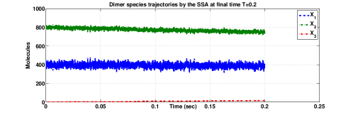
Fig. 1: Trajectories of dimer species trajectories simulated by SSA at the final time, $T=0.2$. This system has multiple timescales. The step size, $\tau^{\text{exp}}$, is therefore taken to be extremely small to ensure the numerical stability of the explicit-TL method ($\tau_{\text{exp}}^{\text{lim}}\approx 2.3\times 10^{-4})$.

Figure (1) shows the trajectories of dimer species with the reaction set (4.1) solved with the original SSA.

4.1.1 Coupling Results

The first step to construct our multilevel hybrid SSI-TL estimator is to check that the coupling procedure is correct in terms of convergence properties. The convergence tests that we did for the coupling algorithm indicate that the global weak convergence and the global convergence of the variance are approximately of order $1$ (see Figures 2 and 3). These results validate our coupling algorithm, which can be used to construct the corresponding MLMC estimator.

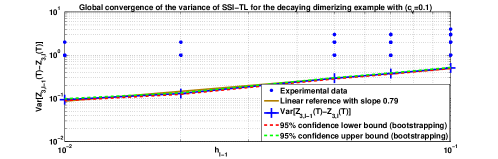
Fig. 2: Global Convergence of the variance of SSI-TL for the decaying dimerizing example. The blue dots correspond to the observed data (each realization of $Z_{3,\ell}-Z_{3,\ell-1}$). We fit $\mathrm{Var}\left[Z_{3,\ell}-Z_{3,\ell-1}\right]$ using a bootstrapping technique [20] with a coefficient of variation, $c_{v}=0.1$. There are some outliers due to the large kurtosis problem (see Section 1 of [36]).

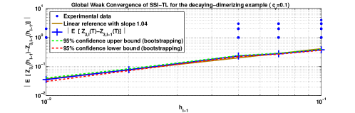
Fig. 3: Global weak convergence SSI-TL for the decaying-dimerizing example. Here, we fit $\mathrm{E}\left[Z_{3,\ell}-Z_{3,\ell-1}\right]$ using a bootstrapping technique with a coefficient of variation, $c_{v}=0.1$.

4.1.2 Multilevel Hybrid SSI-TL Results ($L\leq L_{c}^{\text{exp}}$)

Now, we compare the performance of our multilevel hybrid SSI-TL algorithm, reduced to the multilevel SSI-TL algorithm when $L\leq L_{c}^{\text{exp}}$, to the performance of the multilevel explicit-TL and MC SSI-TL methods. First, we should mention that to ensure the numerical stability of the multilevel explicit-TL estimator, we should be restricted to the stability limit given by $\tau_{\text{exp}}^{\text{lim}}\approx 2.3\times 10^{-4}$. However, in the implicit case, we do not have any stability restriction. Therefore, in our numerical experiments, we started with $L_{c}^{\text{exp}}=10$ for the multilevel explicit-TL estimator ($L_{c}^{\text{exp}}$ satisfies $h_{L_{c}^{\text{exp}}}=2^{-L_{c}^{\text{exp}}}T<2.3\times 10^{-4}$). We also varied the prescribed tolerance, $TOL$, to investigate its effect on the performance of the tested methods.

The finest level of discretization, $L$, given in Figure 6, is obtained by extrapolating the weak error and deduced from Figures 4 and 5 . The value of the finest level satisfies $Bias(L)<\frac{TOL}{2}$. From Figure 6, we notice that to achieve the same weak error, we use seven more levels for the explicit-TL compared to those for SSI-TL . As a consequence, the weak error for the implicit scheme is a factor of $2^{7}=128$ smaller than for the explicit method. Even though this high gain in discretization is deteriorated by the additional cost of Newton iterations at each level, it is still one of the main factors that explains the great advantage of the multilevel SSI-TL over the explicit version as we will see later.

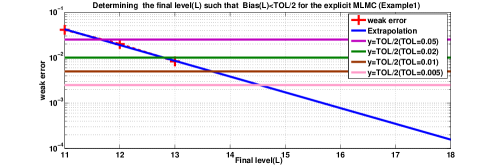
Fig. 4: Determining the final level (L) such that $Bias(L)<TOL/2$ for the multilevel explicit-TL (Example 1). We estimate the bias for small values of level $\ell$ and then we extrapolate to obtain final level $L$.

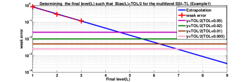
Fig. 5: Determining the final level(L) such that $Bias(L)<TOL/2$ for the multilevel SSI-TL (Example 1).

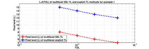
Fig. 6: The finest level (L) as a function of tolerance, $TOL$, for multilevel SSI-TL and multilevel explicit-TL methods for Example 1. These values are obtained as a result of figures (4 and 5).

The variances, $\{V_{\ell}\}_{\ell=L_{c}^{\text{imp}}=0}^{L^{\text{imp}}}$, used in the optimization problem (25) are obtained by the extrapolation of the estimated variances of the first three levels and given in Table 2.

explicit-TL		SSI-TL
level	variance	level	variance
$11$	$4.1\times 10^{-2}$	$1$	$3.1$
$12$	$1.9\times 10^{-2}$	$2$	$1.7$
$13$	$8.2\times 10^{-3}$	$3$	$9\times 10^{-1}$
$14$	$3.7\times 10^{-3}$	$4$	$4.9\times 10^{-1}$
$15$	$1.6\times 10^{-3}$	$5$	$2.6\times 10^{-1}$
$16$	$7\times 10^{-4}$	$6$	$1.4\times 10^{-1}$
$17$	$3\times 10^{-4}$	$7$	$7.7\times 10^{-2}$
$18$	$10^{-4}$	$8$	$4.1\times 10^{-2}$

Table 2: Extrapolation for the estimated variances, $\mathrm{Var}\left[Z_{\ell,3}-Z_{\ell-1,3}\right]\>(\ell=11,12,13)$ for the multilevel explicit-TL and $(\ell=1,2,3)$ for multilevel SSI-TL (Example 1).

To obtain the optimal number of samples per level for the multilevel SSI-TL estimator, we followed the procedure described in Section 3.3 and our numerical results are presented in Tables 7 and 8 in the Appendix. These tables show the optimal number of samples for each estimator per level and for different values of tolerances, $TOL=\{0.05,\>0.02,\>0.01,\>0.005\}$. From the previous tables and Figure 7, we see that the optimal number of samples increases as we decrease the tolerance. It decreases with respect to the level, $\ell$, due to the decrease in both $V_{\ell}$ and $h_{\ell}$. We also mention that the value of the finest level, $L$, the maximum level of time step refinement, increases as the value of the tolerance decreases. The control-variate technique that we used allowed us to reduce the number of samples at the coarsest level by a factor of six (see Tables 8 and 9).

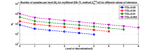
Fig. 7: Optimal number of samples per level for the multilevel SSI-TL method ($L_{c}^{\text{imp}}=0$) for Example 1. These values are obtained by solving the optimization problem (25). The optimal number of samples increases as we decrease the tolerance. It decreases with respect to the level, $\ell$, due to the decrease of both $V_{\ell}$ and $h_{\ell}$. Note that the value of the finest level, $L$, the maximum level of time step refinement, increases as the value for the tolerance decreases.

To compare the computational work of the different methods, $100$ sets of multilevel calculations were performed for each value of tolerance, $TOL$. The actual work (runtime) was obtained using a 12-core Intel GLNXA64 architecture and MATLAB version R2014a. The results, given in Table 3, indicate that we achieve the lowest computational cost using the multilevel SSI-TL estimator, which outperforms by about three times both the multilevel explicit-TL estimator and the MC SSI-TL estimator in terms of computational work. In addition, Figure 8 shows that we achieve computational work, $W$, of ${\mathcal{O}}\left(TOL^{-2}(\log(TOL))^{2}\right)$ for both multilevel SSI-TL and multilevel explicit-TL methods. This result confirms the computational advantage of MLMC over MC.

Method / TOL	$0.05$	$0.02$	$0.01$	$0.005$
Multilevel explicit-TL	500 (7)	3900 (21)	1.7+e04 (80)	8.6+e04 (570)
Multilevel SSI-TL	150 (3)	1300 (15)	5.9+e03 (47)	3.1+e04 (265)
MC SSI-TL	87 (1)	1400 (16)	1.1+e04 (72)	8.9+e04 (589)
$W_{\text{MLMC}}^{\text{exp}}/W_{\text{MLMC}}^{\text{SSI}}$	3.30	2.97	2.85	2.80
$W_{\text{MC}}^{\text{SSI}}/W_{\text{MLMC}}^{\text{SSI}}$	0.58	1.10	1.84	2.91

Table 3: Comparison of the expected total work for the different methods (in seconds) using $100$ multilevel runs for Example 1 $(L_{c}^{\text{exp}}=10\;\text{and}\;L_{c}^{\text{imp}}=0)$. The quantity in parentheses, i.e., $(\cdot)$, refers to the standard deviation. The speedup factors given in the last two rows show that the multilevel SSI-TL performs faster than the multilevel explicit-TL and the MC SSI-TL methods.

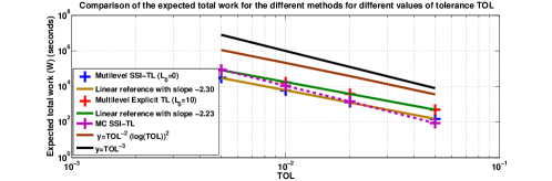
Fig. 8: Comparison of the expected total work for the different methods with different values of tolerance ($TOL$) for Example 1 using $100$ multilevel runs. The computational work, $W$, of both multilevel SSI-TL and multilevel explicit-TL methods is of ${\mathcal{O}}\left(TOL^{-2}(\log(TOL))^{2}\right)$ compared to ${\mathcal{O}}\left(TOL^{-3}\right)$ for the MC SSI-TL method.

This computational gain by the multilevel SSI-TL method over the multilevel explicit-TL method is due to the lower cost of constructing single and coupled paths for the SSI-TL method compared with the explicit one as illustrated by Figure 9. This figure shows that this computational gain, due to using coarse time discretization in the SSI-TL method, deteriorates due to the cost of Newton iterations. This is illustrated by having the same computational cost to generate coupled paths of explicit-TL and SSI-TL while using different time step sizes (comparing the time to generate the coupled paths corresponding to level $\ell=8$ for the SSI-TL and the paths corresponding to level $\ell=13$ for the explicit-TL ). This observation motivated our idea of switching from the multilevel SSI-TL to the multilevel explicit-TL method, particularly when the value of $TOL$ is very small, implying a large value of the finest level of the drift-implicit MLMC, $L^{\text{imp}}$, such that $L^{\text{imp}}\geq L_{c}^{\text{exp}}$ ($L_{c}^{\text{exp}}$ refers to the first level of discretization from which the multilevel explicit-TL method becomes stable).

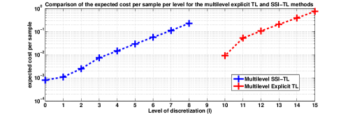
Fig. 9: Comparison of the expected cost per sample per level of the different methods for Example 1 using $10^{5}$ samples. The first observation corresponds to the time of a single path for the coarsest level and the other observations correspond to the time of the coupled paths per level. The computational gain due to using coarse-time discretization for SSI-TL deteriorates due to the cost of Newton iterations as level $\ell$ increases. We note that we use a fixed number of Newton iterations equal to 3.

Remark 4.1.

In future work, we will implement the method entirely in C++ to confirm the computational work gains.

The QQ-plot and probability mass function plot in Figure 10 show, for the smallest considered TOL, $100$ independent realizations of the multilevel SSI-TL estimator. These plots, complemented by a Shapiro-Wilk normality test, validate our assumption about the Gaussian distribution of the statistical error. In Figure (11), we show TOL versus the actual computational error. The prescribed tolerance is achieved with the required confidence of $95\%$.

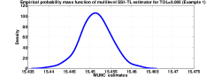
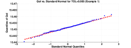
Fig. 10: Left: Empirical probability mass function for $100$ multilevel SSI-TL estimates. Right: QQ-plot for the multilevel SSI-TL estimates in Example 1.

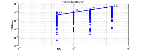
Fig. 11: TOL versus the actual computational error for Example 1. The numbers above the straight line show the percentage of runs that had errors larger than the required tolerance. We observe that in all cases, except for the smallest tolerance, the computational error follows the imposed tolerance with the expected confidence of $95\%.$

4.1.3 Multilevel Hybrid SSI-TL Results ($L\geq L_{c}^{\text{exp}}$)

Here, we show results for our multilevel hybrid SSI-TL estimator for different values of the interface level $L^{\text{int}}$. Table 4 shows that we achieve the lowest computational cost for $L^{\text{int}}=L_{c}^{\text{exp}}$. This can be explained by analyzing the cost per level of the multilevel hybrid SSI-TL estimator (see Figure 14 and using relation (3.3.3)). Table 4 also shows that our estimator outperforms the explicit one by about three times. This gain can be more important for very small values of tolerance, $TOL$. Figure 12 shows the optimal number of samples in our SSI-TL setting. We observe jumps at the interface level, $L^{\text{int}}$, which are a consequence of jumps in the variance of the coupled paths. This is due to the fact that the variance of coupled paths, for the same discretization level, simulated by the SSI-TL is smaller than the variance simulated either by the explicit or the coupling of the SSI-TL with the explicit-TL method (see Figure 13).

Method / TOL	$0.01$	$0.005$
Multilevel explicit-TL $(L_{c}^{\text{exp}}=10)$	1.7e+04(80)	8.6e+04 (570)
Multilevel Hybrid SSI-TL $(L_{c}^{\text{imp}}=0,L^{\text{int}}=10)$	7.2e+03 (52)	2.8e+04 (239)
Multilevel Hybrid SSI-TL $(L_{c}^{\text{imp}}=0,L^{\text{int}}=11)$	8.7e+03 (55)	3.2e+04 (271)
Multilevel Hybrid SSI-TL $(L_{c}^{\text{imp}}=0,L^{\text{int}}=12)$	1.1e+04 (69)	3.9e+04 (246)
$W_{\text{MLMC}}^{\text{exp}}/W_{\text{MLMC}}^{\text{hyb}}(L^{\text{int}}=10)$	2.36	3.07

Table 4: Comparison of the expected total work for the different methods (in seconds) using $100$ multilevel runs for Example 1. The quantity in parentheses refers to the standard deviation. The optimal value of the interface level is $L^{\text{int}}=L_{c}^{\text{exp}}$. The speedup factor, represented by the last row, can reach a factor of $3$.

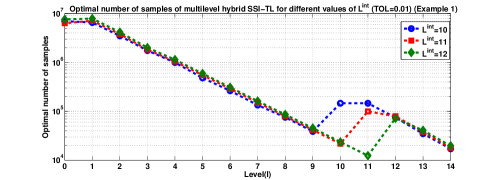
Fig. 12: Optimal number of samples of multilevel hybrid SSI-TL estimator for different values of $L^{\text{int}}$ ($TOL=0.01$) (Example 1). We observe jumps at the interface level, $L^{\text{int}}$.

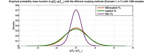
Fig. 13: Empirical probability mass function of $g(\mathbf{Z}_{\ell})-g(\mathbf{Z}_{\ell-1})$ simulated by the different coupling methods (Example 1, $\ell=11$) with $10^{3}$ samples. The variance of the difference between coupled paths simulated by the SSI-TL method is smaller than the variance simulated either by the explicit or the coupling of the SSI-TL with the explicit-TL method.

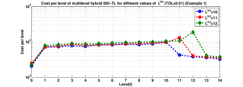
Fig. 14: Cost per level of the multilevel hybrid SSI-TL estimator for different values of $L^{\text{int}}$ ($TOL=0.01$) (Example 1). This figure explains why the lowest computational cost is most likely to be achieved for $L^{\text{int}}=L_{c}^{\text{exp}}$ (see analysis in Section 3.3).

4.2 Example 2

This example was studied in [40] and is given by the following reaction set

$$S_{1} \overset{c_{1}}{\rightarrow}S_{3},$$

$$S_{3} \overset{c_{2}}{\rightarrow}S_{1}$$

(29) $$S_{1}+S_{2} \overset{c_{3}}{\rightarrow}S_{1}+S_{4}.$$

Since the total number of $S_{1}$ and $S_{3}$ molecules is constant (say $K$), and since we can ignore the by-product, $S_{4}$, this system can be represented by three reactions and two variables, $\mathbf{X}=(X_{1},X_{2})$, which are numbers of $S_{1}$ and $S_{2}$ molecules, respectively. The stoichiometric vectors are $\boldsymbol{\nu}_{1}=(-1,0)^{T}$, $\boldsymbol{\nu}_{2}=(1,0)^{T}$, and $\boldsymbol{\nu}_{3}=(0,-1)^{T}$ and the corresponding propensity functions are

(30) $$a_{1}(\mathbf{X})=c_{1}X_{1},\>a_{2}(\mathbf{X})=c_{2}(K-X_{1}),\>a_{3}(\mathbf{X})=c_{3}X_{1}X_{2}.$$

We chose the same values for the different parameters as in [40]: $c_{1}=c_{2}=10^{5}$, $c_{3}=5\times 10^{-3}$, $K=2\times 10^{4}$ and initial condition $\mathbf{X}(0)=(10^{4},10^{2})^{T}$. This setting implies that the stability limit of the explicit-TL is $\tau_{\text{exp}}^{\text{lim}}\approx 10^{-5}$. We consider the final time, $T=0.01$ seconds. In the following numerical experiments, we are interested in approximating $\mathrm{E}\left[X_{2}(T)\right]$.

4.2.1 Multilevel SSI-TL Results ($L\leq L_{c}^{\text{exp}}$)

Similarly to what we did in the first example, we checked whether the coupling procedure is reliable in terms of convergence properties and we followed the same steps shown in Example 1. Now, we want to compare the performance of our multilevel hybrid SSI-TL algorithm, reduced to the multilevel SSI-TL algorithm when $L\leq L_{c}^{\text{exp}}$, to the performance of the multilevel explicit-TL and MC SSI-TL methods. Here, we fix $L_{c}^{\text{exp}}=11$ for the multilevel explicit-TL estimator to ensure the numerical stability ($2^{-L_{c}^{\text{exp}}}T<10^{-5}$). We also vary the prescribed tolerance, $TOL$, to investigate its effect on the performance of the tested methods. We note that, in this example, we use a fixed number of Newton iterations equal to 3 for the SSI-TL method.

To compare the computational work of the different methods, $100$ sets of multilevel calculations were performed for each value of tolerance $TOL$. The results presented in Table 5 and Figure 15 indicate that we achieve the lowest computational cost with the multilevel SSI-TL estimator, which outperforms by about $40$ times the multilevel explicit-TL estimator and by about $11$ times the MC SSI-TL estimator in terms of computational work. Similarly to the first example, Figure 8 shows that we achieve computational work, $W$, of ${\mathcal{O}}\left(TOL^{-2}(\log(TOL))^{2}\right)$ for both multilevel SSI-TL and multilevel explicit-TL methods. This result confirms the computational advantage of MLMC over MC.

Method / TOL	$0.04$	$0.02$	$0.01$	$0.005$
Multilevel explicit-TL	170 (4)	890 (9)	5300 (45)	2.2e+04 (96)
Multilevel SSI-TL	5 (0.2)	240 (0.8)	110 (3)	5.3e+02 (7)
MC SSI-TL	18 (0.6)	140 (3)	770 (8)	6e+03 (48)
$W_{\text{MLMC}}^{\text{exp}}/W_{\text{MLMC}}^{\text{SSI}}$	33.40	37.04	47.33	41.27
$W_{\text{MC}}^{\text{SSI}}/W_{\text{MLMC}}^{\text{SSI}}$	3.60	5.70	6.84	11.37

Table 5: Comparison of the expected total work for the different methods (in seconds) using $100$ multilevel runs for Example 2 $(L_{c}^{\text{exp}}=11\>\>\text{and}\>\>L_{c}^{\text{imp}}=0)$. The quantity in parentheses refers to the standard deviation. The speedup factors are more important in this example. From the last two rows, we notice that the multilevel SSI-TL estimator outperforms by about $40$ times the multilevel explicit-TL estimator and by about $11$ times the MC SSI-TL estimator in terms of computational work.

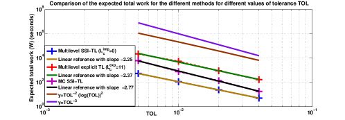
Fig. 15: Comparison of the expected total work for the different methods with different values of tolerance ($TOL$) for Example 2 using $100$ multilevel runs. The computational work, $W$, of both multilevel SSI-TL and multilevel explicit-TL methods is ${\mathcal{O}}\left(TOL^{-2}(\log(TOL))^{2}\right)$ compared to ${\mathcal{O}}\left(TOL^{-3}\right)$ for the MC SSI-TL .

This computational gain of the multilevel SSI-TL method over the multilevel explicit-TL method is, as in the previous example, due to the lower cost of constructing single and coupled paths by SSI-TL compared to the cost by the explicit method as illustrated by Figure 16. Similarly to the first example, we can notice from this figure that the computational gain due to using coarse-time discretization for the SSI-TL method deteriorates due to the cost of Newton iterations.

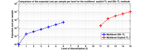
Fig. 16: Comparison of the expected cost per sample per level for the different methods for Example 2 using $10000$ samples. The first observation corresponds to the time of a single path for the coarsest level and the other observations correspond to the time of the coupled paths per level.

The QQ-plot and probability mass function plot in Figure 17 show, for the smallest considered TOL, $100$ independent realizations of the multilevel SSI-TL estimator. These plots, complemented with a Shapiro-Wilk normality test, validates our assumption about the Gaussian distribution of the statistical error. In Figure 18, we show TOL versus the actual computational error. The prescribed tolerance is achieved with the required confidence of $95\%$.

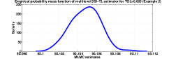
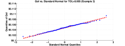
Fig. 17: Left: Empirical probability mass function for $100$ multilevel SSI-TL estimates. Right: QQ-plot for the multilevel SSI-TL estimates in Example 2.

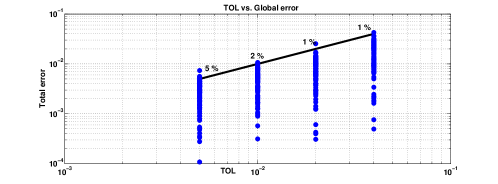
Fig. 18: TOL versus the actual computational error for Example 2. The numbers above the straight line show the percentage of runs that had errors larger than the required tolerance. We observe that in all cases, except for the smallest tolerance, the computational error follows the imposed tolerance with the expected confidence of $95\%.$

4.2.2 Multilevel Hybrid SSI-TL Results ($L\geq L_{c}^{\text{exp}}$)

Here, we present the results of the multilevel hybrid SSI-TL estimator for different values of the interface level $L^{\text{int}}$. Table 6 shows that we achieve the lowest computational cost for, $L^{\text{int}}=L_{c}^{\text{exp}}$. This can be explained by analyzing the cost per level of the multilevel hybrid SSI-TL estimator (see Figure 20 and using relation (3.3.3)). Table 6 also shows that our multilevel estimator outperforms the explicit one by about seven times. This gain can be more important for very small values of tolerance, $TOL$. Figure 19 shows the optimal number of samples in the SSI-TL setting. We observe jumps at the interface level, $L^{\text{int}}$, which are a consequence of jumps in the variance of the coupled paths.

Method / TOL	$0.01$	$0.005$
Multilevel explicit-TL $(L_{c}^{\text{exp}}=11)$	5.3e+03 (45)	2.2e+04 (96)
Multilevel Hybrid SSI-TL $(L_{c}^{\text{imp}}=0,L^{\text{int}}=11)$	9.4e+02 (11)	3.2e+03 (15)
Multilevel Hybrid SSI-TL $(L_{c}^{\text{imp}}=0,L^{\text{int}}=12)$	9.9e+02 (12)	3.3e+03 (15)
Multilevel Hybrid SSI-TL $(L_{c}^{\text{imp}}=0,L^{\text{int}}=13)$	1.3e+03 (13)	3.6e+03 (19)
$W_{\text{MLMC}}^{\text{exp}}/W_{\text{MLMC}}^{\text{hyb}}(L^{\text{int}}=11)$	5.64	6.87

Table 6: Comparison of the expected total work for the different methods (in seconds) using $100$ multilevel runs for Example 2. The quantity in parentheses refers to the standard deviation. The optimal value of the interface level is $L^{\text{int}}=L_{c}^{\text{exp}}$. The speedup factor, given in the last row, can reach a factor of $7$.

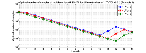
Fig. 19: Optimal number of samples of multilevel hybrid SSI-TL for different values of $L^{\text{int}}$ ($TOL=0.01$) (Example 2). We observe jumps at the interface level, $L^{\text{int}}$.

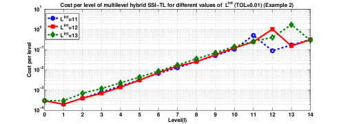
Fig. 20: Cost per level of the multilevel hybrid SSI-TL estimator for different values of $L^{\text{int}}$ ($TOL=0.01$) (Example 2). This figure explains why the lowest computational cost is most likely to be achieved for $L^{\text{int}}=L_{c}^{\text{exp}}$ (see analysis in Section 3.3).

Remark 4.2.

As we argued in the introduction, from Figure 21, we check that simulating single paths with the SSI-TL method is more computationally efficient than with the $\tau$-ROCK method, especially in the case of large time steps.

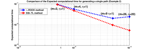
Fig. 21: Comparison between the SSI-TL and the $\tau$-ROCK methods in terms of the expected computational time, using $10^{5}$ samples, for generating a single path (Example 2 in Section 4). The parameters $m$ ( the stage number that controls the stability region) and $\eta$ (the damping parameter that controls the damping effect of the variance) are chosen in such a way that we obtain nearly optimal work for the $\tau$-ROCK method except for $\tau=10^{-3}$. For the sake of comparison, we also show the same values given in [3]

.

5 Conclusions and Future Work

In this work, we adapt the idea of split-step backward-Euler [28] for Brownian SDEs to SDEs driven by Poisson random measures. We extend the SSI-TL idea to the multilevel setting and introduce the multilevel hybrid SSI-TL estimator with the aim of reducing the computational work needed to produce an estimate of $\mathrm{E}\left[g(\mathbf{X}(T))\right]$, within a fixed tolerance, $TOL$, with a given level of confidence. Our estimator couples SSI-TL paths at the coarser discretization levels until a certain interface level, $L^{\text{int}}$, is reached. The $L^{\text{int}}$ level can be reached or not, depending on user-selected tolerance requirements. When the required number of levels is greater than $L^{\text{int}}$, our estimator couples explicit-TL paths at the finer levels and can be even become unbiased by coupling the finest level with a modified next reaction method [7].

Our proposed estimator is useful in systems with the presence of slow and fast timescales (stiff systems). In such situations, the multilevel estimator given in [6] is not computationally efficient due to numerical stability constraints. Through our numerical experiments, we obtained substantial gains with respect to both the multilevel explicit-TL and the single-level SSI-TL methods. We also showed, that for large values of $TOL$, the multilevel hybrid SSI-TL method has the same order of computational work as does the multilevel explicit-TL method, which is of ${\mathcal{O}}\left(TOL^{-2}\log(TOL)^{2}\right)$ [10], but with a smaller constant. Although it is possible to obtain a computational work of ${\mathcal{O}}\left(TOL^{-2}\right)$ by coupling with a pathwise exact path at the deepest level, this is of little help in the class of stiff problems due to the high number of exact steps. As we stressed in Section 3.3, one potential direction of future research is applying the CMLMC algorithm, introduced in [18], in our context. In fact, it may provide an optimal split between bias and statistical errors, implying an improvement in the the computational complexity of our MLMC estimator. Future extensions may also involve hybridization techniques involving methods that deal with non-negativity of species (see [36]). These hybridization techniques can be improved by using the idea of adaptivity introduced in [35, 32], which allows us to construct adaptive hybrid multilevel estimators by switching between SSI-TL , explicit-TL and exact SSA within the course of a single sample. We also intend to extend the $\tau$-ROCK method [3] to the multilevel setting and compare it with the multilevel hybrid SSI-TL method. The main challenge of this task is to couple two consecutive paths based on the $\tau$-ROCK method. Finally, our techniques can be extended to the context of spatial inhomogeneities described, for instance, by graphs and/or continuum volumes.

Appendix A Results of MLMC for Example 1

Level / tol	$0.05$	$0.02$	$0.01$	$0.005$
$15$	-	-	-	$2.5\times 10^{4}$
$14$	-	-	$3.6\times 10^{4}$	$5.3\times 10^{4}$
$13$	-	$1.8\times 10^{4}$	$7.3\times 10^{4}$	$3.1\times 10^{5}$
$12$	$4.5\times 10^{3}$	$3.4\times 10^{4}$	$1.4\times 10^{5}$	$5.3\times 10^{5}$
$11$	$9.6\times 10^{3}$	$7.9\times 10^{4}$	$3.3\times 10^{5}$	$1.3\times 10^{6}$
$10$	$1.6\times 10^{5}$	$1.2\times 10^{6}$	$5.0\times 10^{6}$	$2.1\times 10^{7}$

Table 7: Optimal number of samples per level for the multilevel explicit-TL for example 1 $(L_{0}=10)$

Level / tol	$0.05$	$0.02$	$0.01$	$0.005$
$8$	-	-	-	$2.0\times 10^{5}$
$7$	-	-	$8.7\times 10^{4}$	$3.9\times 10^{5}$
$6$	-	$3.5\times 10^{4}$	$1.7\times 10^{5}$	$7.3\times 10^{5}$
$5$	$8.8\times 10^{3}$	$7.0\times 10^{4}$	$3.1\times 10^{5}$	$1.4\times 10^{6}$
$4$	$1.7\times 10^{4}$	$1.3\times 10^{5}$	$6.1\times 10^{5}$	$2.7\times 10^{6}$
$3$	$3.3\times 10^{4}$	$2.6\times 10^{5}$	$10^{6}$	$5.2\times 10^{6}$
$2$	$5.8\times 10^{4}$	$4.6\times 10^{5}$	$1.9\times 10^{6}$	$9.3\times 10^{6}$
$1$	$1.2\times 10^{5}$	$9.4\times 10^{5}$	$3.9\times 10^{6}$	$1.9\times 10^{7}$
$0$	$6.7\times 10^{5}$	$3.5\times 10^{6}$	$2.4\times 10^{7}$	$10^{8}$

Table 8: Optimal number of samples per level for the multilevel SSI-TL for example 1 $(L_{0}=0)$

Level / tol	$0.05$	$0.02$	$0.01$	$0.005$
$8$	-	-	-	$1.9\times 10^{5}$
$7$	-	-	$7.7\times 10^{4}$	$3.6\times 10^{5}$
$6$	-	$3.1\times 10^{4}$	$1.5\times 10^{5}$	$6.7\times 10^{5}$
$5$	$8.0\times 10^{3}$	$6.1\times 10^{4}$	$2.9\times 10^{5}$	$1.3\times 10^{6}$
$4$	$1.6\times 10^{4}$	$1.2\times 10^{5}$	$5.5\times 10^{5}$	$2.6\times 10^{6}$
$3$	$2.8\times 10^{4}$	$2.1\times 10^{5}$	$10^{6}$	$4.6\times 10^{6}$
$2$	$5.7\times 10^{4}$	$4.4\times 10^{5}$	$2.0\times 10^{6}$	$10^{7}$
$1$	$1.1\times 10^{5}$	$8.5\times 10^{5}$	$3.9\times 10^{6}$	$1.9\times 10^{7}$
$0$	$1.1\times 10^{5}$	$8.1\times 10^{5}$	$4.0\times 10^{6}$	$1.7\times 10^{7}$

Table 9: Optimal number of samples per level for the multilevel SSI-TL for example 1 with control-variate technique.

tol	$0.5$	$0.2$	$0.1$	$0.05$
Needed number of samples	$1.3\times 10^{5}$	$10^{6}$	$4.2\times 10^{6}$	$1.7\times 10^{7}$

Table 10: Needed number of samples for the MC SSI-TL for Example 1.

References

- [1] A. Abdulle and S. Cirilli. Stabilized methods for stiff stochastic systems. Comptes Rendus Mathematique, 345(10):593–598, 2007.
- [2] A. Abdulle and S. Cirilli. S-rock: Chebyshev methods for stiff stochastic differential equations. SIAM Journal on Scientific Computing, 30(2):997–1014, 2008.
- [3] A. Abdulle, Y. Hu, and T. Li. Chebyshev methods with discrete noise: the tau-rock methods. J. Comput. Math, 28(2):195–217, 2010.
- [4] A. Abdulle and T. Li. S-rock methods for stiff sdes. Commun. Math. Sci., 6(4):845–868, 12 2008.
- [5] T. Ahn, A. Sandu, and X. Han. Implicit simulation methods for stochastic chemical kinetics. CoRR, abs/1303.3614, 2013.
- [6] D. Anderson and D. Higham. Multilevel Monte Carlo for continuous Markov chains, with applications in biochemical kinetics. SIAM Multiscal Model. Simul., 10(1), 2012.
- [7] D. F. Anderson. A modified next reaction method for simulating chemical systems with time dependent propensities and delays. The Journal of Chemical Physics, 127(21):214107, 2007.
- [8] D. F. Anderson. Incorporating postleap checks in tau-leaping. The Journal of chemical physics, 128(5):054103, 2008.
- [9] D. F.Anderson, A. Ganguly, and T. G.Kurtz. Error analysis of tau-leap simulation methods The Annals of Applied Probability., 2226–2262, 2011.
- [10] D. F. Anderson, D. J. Higham, and Y. Sun. Complexity of multilevel Monte Carlo tau-leaping. SIAM Journal on Numerical Analysis, 52(6):3106–3127, 2014.
- [11] D. F. Anderson and T. G. Kurtz. Stochastic analysis of biochemical systems. Springer, 2015.
- [12] F. Brauer and C. Castillo-Chavez. Mathematical Models in Population Biology and Epidemiology (Texts in Applied Mathematics). Springer, 2nd edition, 2011.
- [13] E. Cinlar. Probability and stochastics, volume 261 of Graduate texts in Mathematics. Springer, 2011.
- [14] Y. Cao, D. T. Gillespie, and L. R. Petzold. Avoiding negative populations in explicit Poisson tau-leaping. Journal of Chemical Physics, 123(5):054104+, Aug. 2005.
- [15] Y. Cao, D. T. Gillespie, and L. R. Petzold. Efficient step size selection for the tau-leaping simulation method. The Journal of Chemical Physics, 124(4):044109, 2006.
- [16] Y. Cao and L. Petzold. Trapezoidal tau-leaping formula for the stochastic simulation of biochemical systems. In Foundations of Systems Biology in Engineering (FOSBE), pages 149–152, 2005.
- [17] Y. Cao, L. Petzold, M. Rathinam, and D. Gillespie. The numerical stability of leaping methods for stochastic simulation of chemically reacting systems. Journal of Chemical Physics, 121(24):12169–12178, DEC 22 2004.
- [18] N. Collier, A.-L. Haji-Ali, F. Nobile, E. von Schwerin, and R. Tempone. A continuation multilevel Monte Carlo algorithm. BIT Numerical Mathematics, 55(2):399–432, 2014.
- [19] D. Duffie and P. Glynn. Efficient Monte Carlo simulation of security prices. The Annals of Applied Probability, pages 897–905, 1995.
- [20] B. Efron and R. J. Tibshirani. An Introduction to the Bootstrap. Chapman & Hall, New York, 1993.
- [21] S. Engblom. On the stability of stochastic jump kinetics. Appl. Math., 5:3217–3239, 2014.
- [22] S. N. Ethier and T. G. Kurtz. Markov Processes: Characterization and Convergence (Wiley Series in Probability and Statistics). Wiley-Interscience, 2nd edition, 9 2005.
- [23] M. Giles. Multi-level Monte Carlo path simulation. Operations Research, 53(3):607–617, 2008.
- [24] D. T. Gillespie. A general method for numerically simulating the stochastic time evolution of coupled chemical reactions. Journal of Computational Physics, 22:403–434, 1976.
- [25] D. T. Gillespie. Approximate accelerated stochastic simulation of chemically reacting systems. Journal of Chemical Physics, 115:1716–1733, July 2001.
- [26] A. Gupta, C. Briat, and M. Khammash. A scalable computational framework for establishing long-term behavior of stochastic reaction networks. PLOS Computational Biology, 10(6):e1003669, 2014.
- [27] S. Hensel, J. Rawlings, and J. Yin. Stochastic kinetic modeling of vesicular stomatitis virus intracellular growth. Bulletin of Mathematical Biology, 71(7):1671–1692, 2009.
- [28] D. J. Higham, X. Mao, and A. M. Stuart. Strong convergence of Euler-type methods for nonlinear stochastic differential equations SIAM Journal on Numerical Analysis.,40(3):1041–1063, 2002.
- [29] Y. Hu, T. Li, and B. Min. The weak convergence analysis of tau-leaping methods: revisited Commun Math Sci., 2011.
- [30] H. S. J. Aparicio. Population dynamics: Poisson approximation and its relation to the Langevin process. Physical Review Letters, page 4183, 2001.
- [31] P. E. Kloeden and E. Platen. Numerical Solution of Stochastic Differential Equations. Springer, New York, corrected edition, June 2011.
- [32] C. Lester, C. A. Yates, M. B. Giles, and R. E. Baker. An adaptive multi-level simulation algorithm for stochastic biological systems. The Journal of chemical physics, 142(2):024113, 2015.
- [33] T. Li. Analysis of explicit tau-leaping schemes for simulating chemically reacting systems Multiscale Modeling & Simulation., 6(2):417–436, 2007.
- [34] A. Moraes, R. Tempone, and P. Vilanova. Hybrid Chernoff tau-leap. Multiscale Modeling & Simulation, 12(2):581–615, 2014.
- [35] A. Moraes, R. Tempone, and P. Vilanova. Multilevel adaptive reaction-splitting simulation method for stochastic reaction networks. preprint arXiv:1406.1989, 2015.
- [36] A. Moraes, R. Tempone, and P. Vilanova. Multilevel hybrid Chernoff tau-leap. BIT Numerical Mathematics, pages 1–51, 2015.
- [37] M. Rathinam. Moment growth bounds on continuous time Markov processes on non-negative integer lattices. Quart. of Appl. Math., 73:347–364, 2015.
- [38] M. Rathinam. Convergence of moments of tau leaping schemes for unbounded Markov processes on integer lattices SIAM Journal on Numerical Analysis., 54(1):415–439, 2016.
- [39] M. Rathinam, and H. El-Samad. Reversible-equivalent-monomolecular tau: A leaping method for ”small number and stiff” stochastic chemical systems J. Comput. Physics., 224(2):897–923, 2007.
- [40] M. Rathinam, L. Petzold, Y. Cao, and D. T. Gillespie. Stiffness in stochastic chemically reacting systems: the implicit tau-leaping method. Journal of Chemical Physics, 119(24):12784–12794, Dec 2003.
- [41] M. Rathinam, L. R. Petzold, Y. Cao, and D. T. Gillespie. Consistency and stability of tau-leaping schemes for chemical reaction systems. Multiscale Model. Simul., 4(3):867–895 (electronic), 2005.
- [42] R. Srivastava, L. You, J. Summers, and J. Yin. Stochastic vs. deterministic modeling of intracellular viral kinetics. Journal of Theoretical Biology, 218(3):309–321, 2002.
- [43] T. Tian and K. Burrage. Binomial leap methods for simulating stochastic chemical kinetics. J. Chem. Phys., 121(21):10356–10364, 2004.
- [44] Y. Yang, M. Rathinam, and J. Shen. Integral tau methods for stiff stochastic chemical systems J. Chem. Phys., 134(4), 2011.