A Shallow Water Model for Hydrodynamic Processes on Vegetated Hillslope. Water Flow Modulus.

Abstract

The hillslope hydrological processes are very important in watershed hydrology research. In this paper we focus on the water flow over the soil surface with vegetation in a hydrographic basin. We introduce a PDE model based on general principles of fluid mechanics where the unknowns are water depth and water velocity. The influence of the plant cover to the water dynamics is given by porosity (a quantity related to the density of the vegetation), which is a function defined over the hydrological basin. Using finite volume method for approximating the spatial derivatives, we build an ODE system which constitutes the base of the discrete model we will work with. We discuss and investigate several physical relevant properties of this model. Finally, we use numerical results to validate the model.

Keywords: hydrological process, balance equations, shallow water equations, finite volume method, well balanced scheme, porosity

MSC[2010]: 35Q35, 74F10, 65M08

1 Introduction

Mathematical modeling of the hydrodynamic processes in hydrographic basins is of great interest. The subject is very rich in practical applications and there is not yet a satisfactory model to enhance the entire complexity of these processes. However, there are plenty of performant models dedicated to some specific aspects of the hydrodynamic processes only. To review the existent mathematical models is beyond the purposes of this paper, but we can group them into two large classes: physical base models and regression models. The most known regression models are the unit hydrograph [5] and universal soil loss [19, 23]. From the first class, we mention here a few well known models: SWAT [22], SWAP [21] and KINEROS [24]. Due to the complexity and heterogeneity of the processes (see [15]), models in this class are not purely physical because they need additional empirical relations. The main difference between models here is given by the nature of the empirical relations. For example, in order to model the surface of the water flow, SWAP and KINEROS use a mass balance equation and a closure relation, while SWAT combines the mass balance equation with the momentum balance equation. A very special class of models are cellular automata which combine microscale physical laws with empirical closure relations in a specific way to build up a macroscale model, e.g. CAESAR [4, 9].

In this paper, we introduce a physical model described by shallow water type equations. This model is obtained from general principles of fluid mechanics using a space average method and takes into consideration topography, water-soil and water-plant interactions. To numerically integrate the equations, we first apply a finite volume method to approximate the spatial derivatives and then use a type of fractional time-step method to gain the evolution of the water depth and velocity field.

After introducing the PDE model in Section 2, we perform the Finite Volume Method approximation in Section 3 and obtain an ODE [Aversion of Shallow Water Equations. In Section 4, we investigate some physical relevant qualitative properties of this ODE system: monotonicity of the energy, positivity of the water depth function $h$, well balanced properties of the scheme. In Section 5, we obtain the full discrete version of our continuous model; we tackle on the validation method and give some numerical results in the last section.

2 Shalow Water Equations

The model we discuss here is a simplified version a more general model of water flow on a hillslope introduced in [8]. Assume that the soil surface is represented by

$$x^{3}=z(x^{1},x^{2}),\quad(x^{1},x^{2})\in\Omega,$$

and the first derivatives of the function $z(\cdot,\cdot)$ are small quantities. The unknown variables of the model are the water depth $h(t,x)$ and the two components $v_{a}(t,x)$ of the water velocity $\boldsymbol{v}$. The density of the plant cover is quantified by a porosity function $\theta(x)$. The model reads as

$$\begin{array}[]{rl}\partial_{t}\theta h+\partial_{b}(\theta hv^{b})=&\mathfrak{M},\\ \partial_{t}(\theta hv_{a})+\partial_{b}(hv_{a}v^{b})+\theta h\partial_{a}w=&-{\cal K}(h,\theta)|\boldsymbol{v}|v_{a},\quad a=1,2.\end{array}$$ (1)

The term ${\cal K}(h,\theta)|\boldsymbol{v}|v_{a}$ quantifies the interactions water-soil and water-plants [1, 17]. The function ${\cal K}(h,\theta)$ is given by

$${\cal K}(h,\theta)=\alpha_{p}h\left(1-\theta\right)+\theta\alpha_{s},$$ (2)

where $\alpha_{p}$ and $\alpha_{s}$ are two characteristic parameters of the strength of the water-plant and water-soil interactions, respectively. The contribution of rain and infiltration to the water mass balance is taken into account by $\mathfrak{M}$. In (1), $w=g\left[z(x^{1},x^{2})+h\right]$ stands for the free surface level, and $g$ for the gravitational acceleration.

It is important to note that there is an energy function ${\cal E}$ given by

$${\cal E}:=\frac{1}{2}|\boldsymbol{v}|^{2}+g\left(x^{3}+\frac{h}{2}\right)$$ (3)

that satisfies a conservative equation

$$\partial_{t}(\theta h{\cal E})+\partial_{b}\left(\theta hv^{b}\left({\cal E}+g\frac{h}{2}\right)\right)=\mathfrak{M}\left(-\frac{1}{2}|\boldsymbol{v}|^{2}+w\right)-{\cal K}|\boldsymbol{v}|^{3}.$$ (4)

In the absence of the mass source, the system preserves the steady state of a lake

$$\partial_{a}(x^{3}+h)=0,\quad v_{a}=0,\quad a=1,2.$$ (5)

The model (1) is a hyperbolic system of equations with source term, see [11].

Among different features we ask from our approximation scheme, we want the numerical solutions to preserve the lake, the scheme to be well balanced and energetic conservative. These last two properties of a numerical algorithm for the shallow water equation are very important, especially for the case of hydrographic basin applications, because they allow the lake formation and prevent the numerical solution to oscillate in the neighborhood of a lake. In the absence of vegetation, one can find many such schemes, see [3, 18, 6], for example.

3 Finite Volume Method Approximation of 2D Model

Let $\Omega$ be the domain of the space variables $x^{1}$, $x^{2}$ and $\Omega=\cup_{i}\omega_{i},i=\overline{1,N}$ an admissible polygonal partition, [14]. To build a spatial discrete approximation of the model (1), one integrates the continuous equations on each finite volume $\omega_{i}$ and then defines an approximation of the integrals.

Let $\omega_{i}$ be an arbitrary element of the partition. Relatively to it, the integral form of (1) reads as

$$\begin{array}[]{rl}\displaystyle\partial_{t}\int\limits_{\omega_{i}}\theta h{\rm d}x+\int\limits_{\partial\omega_{i}}\theta h\boldsymbol{v}\cdot\boldsymbol{n}{\rm d}s=&\displaystyle\int\limits_{\omega_{i}}\mathfrak{M}{\rm d}x,\\ \displaystyle\partial_{t}\int\limits_{\omega_{i}}\theta hv_{a}{\rm d}x+\int\limits_{\partial\omega_{i}}\theta hv_{a}\boldsymbol{v}\cdot\boldsymbol{n}{\rm d}s+\int\limits_{\omega_{i}}\theta h\partial_{a}w{\rm d}x=&\displaystyle-\int\limits_{\omega_{i}}{\cal K}|\boldsymbol{v}|v_{a}{\rm d}x,\quad a=1,2.\end{array}$$ (6)

Now, we build a discrete version of the integral form by introducing some quadrature formulas. With $\psi_{i}$ standing for some approximation of $\psi$ on $\omega_{i}$, we introduce the approximations

$$\int\limits_{\omega_{i}}\theta h{\rm d}x\approx\sigma_{i}\theta_{i}h_{i},\quad\int\limits_{\omega_{i}}\theta hv_{a}{\rm d}x\approx\sigma_{i}\theta_{i}h_{i}v_{a\,i},\quad\int\limits_{\omega_{i}}{\cal K}|\boldsymbol{v}|v_{a}{\rm d}x\approx\sigma_{i}{\cal K}_{i}|\boldsymbol{v}|_{i}v_{a\,i},$$ (7)

where $\sigma_{i}$ denotes the area of the polygon $\omega_{i}$.

For the integrals of the gradient of the free surface, we start from the identity

$$\int\limits_{\omega_{i}}\theta h\partial_{a}w{\rm d}x=-\int\limits_{\omega_{i}}w\partial_{a}\theta h{\rm d}x+\int\limits_{\partial_{i}\omega_{i}}w\theta hn_{a}{\rm d}s.$$ (8)

Assume that $w$ is constant and equal to $w_{i}$ on $\omega_{i}$ to approximate the first integral on the r.h.s. of (8). Then, we obtain:

$$\int\limits_{\omega_{i}}\theta h\partial_{a}w{\rm d}x\approx\int\limits_{\partial_{i}\omega_{i}}(w-w_{i})\theta hn_{a}{\rm d}s.$$ (9)

Note that if $\omega_{i}$ is a regular polygon and $w_{i}$ is the cell-centered value of $w$, then the approximation is of second order accuracy for smooth fields and it preserves the null value in the case of constant fields $w$.

We introduce the notation

$$\widetilde{\psi}|_{\partial\omega(i,j)}:=\int\limits_{\partial\omega(i,j)}\psi{\rm d}s.$$ (10)

Using the approximations (7) and (9) and keeping the boundary integrals, one can write

$$\begin{array}[]{rl}\sigma_{i}\partial_{t}\theta_{i}h_{i}+\sum\limits_{j\in{\cal N}(i)}\widetilde{\theta hv_{n}}|_{\partial\omega(i,j)}=&\sigma_{i}\mathfrak{M}_{i},\\ \sigma_{i}\partial_{t}\theta_{i}h_{i}v_{a\,i}+\sum\limits_{j\in{\cal N}(i)}\widetilde{\theta hv_{a}v_{n}}|_{\partial\omega(i,j)}+\sum\limits_{j\in{\cal N}(i)}\widetilde{(w-w_{i})\theta h}n_{a}|_{\partial\omega(i,j)}=&-\sigma_{i}{\cal K}_{i}|\boldsymbol{v}|_{i}v_{a\,i},\end{array}$$ (11)

where ${\cal N}(i)$ denotes the set of all the neighbors of $\omega_{i}$ and $\partial\omega(i,j)$ is the common boundary of $\omega_{i}$ and $\omega_{j}$.

The next step is to define the approximations of the boundary integrals in (11). We approximate an integral $\widetilde{\psi}|_{\partial\omega(i,j)}$ of the form (10) by considering the integrand $\psi$ to be a constant function $\psi_{(i,j)}(\psi_{i},\psi_{j})$, where $\psi_{i}$ and $\psi_{j}$ are some fixed values of $\psi$ on the adjacent cells $\omega_{i}$ and $\omega_{j}$, respectively. Thus,

$$\begin{array}[]{l}\widetilde{\theta hv_{n}}|_{\partial\omega(i,j)}\approx l_{(i,j)}\theta h_{(i,j)}(v_{n})_{(i,j)},\\ \widetilde{\theta hv_{a}v_{n}}|_{\partial\omega(i,j)}\approx l_{(i,j)}\theta h_{(i,j)}(v_{a})_{(i,j)}(v_{n})_{(i,j)},\\ \widetilde{(w-w_{i})\theta h}n_{a}|_{\partial\omega(i,j)}\approx l_{(i,j)}(w_{(i,j)}-w_{i})\theta h^{s}_{(i,j)}(n_{a})_{(i,j)},\end{array}$$ (12)

where $\boldsymbol{n}_{(i,j)}$ denotes the unitary normal to the common side of $\omega_{i}$ and $\omega_{j}$ pointing towards $\omega_{j}$, and $l_{(i,j)}$ is the length of this common side.

The issue is to define the interface value functions $\psi_{(i,j)}(\psi_{i},\psi_{j})$ so that the resulting scheme is well balanced and energetically stable.

Well balanced and energetically stable scheme. For any internal interface $(i,j)$, we define the following quantities:

$$\begin{array}[]{l}(v_{a})_{(i,j)}=\displaystyle\frac{v_{a\,i}+v_{a\,j}}{2},\quad a=1,2,\\ (v_{n})_{(i,j)}=\boldsymbol{v}_{(i,j)}\cdot\boldsymbol{n}_{(i,j)},\\ w_{(i,j)}=\displaystyle\frac{w_{i}+w_{j}}{2},\end{array}$$ (13)

and

$$\theta h^{s}_{(i,j)}=\left\{\begin{array}[]{ll}\theta h_{(i,j)},&{\rm if}\;(v_{n})_{(i,j)}\neq 0,\\ \theta_{i}h_{i},&{\rm if}\;(v_{n})_{(i,j)}=0\;{\rm and}\;w_{i}>w_{j},\\ \theta_{j}h_{j},&{\rm if}\;(v_{n})_{(i,j)}=0\;{\rm and}\;w_{i}\leq w_{j}.\end{array}\right.$$ (14)

$h$-positivity. In order to preserve the positivity of $h$, we define $\theta h_{(i,j)}$ as

$$\theta h_{(i,j)}=\left\{\begin{array}[]{ll}\theta_{i}h_{i},&{\rm if}\;(v_{n})_{(i,j)}>0,\\ \theta_{j}h_{j},&{\rm if}\;(v_{n})_{(i,j)}<0.\end{array}\right.$$ (15)

The semidiscrete scheme takes now the form of the following system of ODEs

$$\begin{array}[]{rl}\sigma_{i}\displaystyle\frac{\rm d}{{\rm d}t}\theta_{i}h_{i}+\sum\limits_{j\in{\cal N}(i)}l_{(i,j)}\theta h_{(i,j)}(v_{n})_{(i,j)}=&\sigma_{i}\mathfrak{M}_{i},\\ \sigma_{i}\displaystyle\frac{\rm d}{{\rm d}t}\theta_{i}h_{i}v_{a\,i}+\sum\limits_{j\in{\cal N}(i)}l_{(i,j)}\theta h_{(i,j)}(v_{a})_{(i,j)}(v_{n})_{(i,j)}+&\\ +\displaystyle\frac{1}{2}\sum\limits_{j\in{\cal N}(i)}l_{(i,j)}(w_{j}-w_{i})(\theta h)^{s}_{(i,j)}n_{a}|_{(i,j)}&=-\sigma_{i}{\cal K}_{i}|\boldsymbol{v}|_{i}v_{a\,i}.\end{array}$$ (16)

Boundary conditions. Free discharge. We need to define the values of $h$ and $\boldsymbol{v}$ on the external sides of $\Omega$. For each side in $\Gamma=\partial\Omega$ we introduce a new cell (“ghost” element) adjacent to the polygon $\omega_{i}$ corresponding to that side. For each “ghost” element, one must somehow define its altitude and then we set zero values to its water depth. We can now define $h$ and $\boldsymbol{v}$ on the external sides of $\Omega$ by

$$\begin{array}[]{l}\boldsymbol{v}_{\partial\omega_{i}\cap\Gamma}=\boldsymbol{v}_{i},\\ h_{\partial\omega_{i}\cap\Gamma}=\left\{\begin{array}[]{ll}h_{i},&{\rm if}\;\boldsymbol{v}_{i}\cdot\boldsymbol{n}|_{\partial\omega_{i}\cap\Gamma}>0,\\ 0,&{\rm if}\;\boldsymbol{v}_{i}\cdot\boldsymbol{n}|_{\partial\omega_{i}\cap\Gamma}<0.\end{array}\right.\end{array}$$ (17)

Now, the solution is sought inside the positive cone $h_{i}>0,\;i=\overline{1,N}$.

4 Properties of the semidiscrete scheme

The ODE model (16) can have discontinuities in the r.h.s. and therefore it is possible that the solution in the classical sense of this system might not exist for some initial data. However, the solution in Filipov sense [7] exists for any initial data.

There are initial data for which the solution in the classical sense exists only locally in time. Since the numerical scheme is a time approximation of the semidiscrete form (16), it is worthwhile to analyze the properties of these classical solutions. Numerical schemes preserving properties of some particular solutions of the continuum model were and are intensively investigated in the literature [2, 3, 6, 16]. In the present section we investigate such properties for the semidiscrete scheme and the next section is dedicated to the properties of the complete discretized scheme.

4.1 Energy balance

Definition (13) yields a dissipative conservative equation for the cell energy ${\cal E}_{i}$,

$${\cal E}_{i}(h_{i},\boldsymbol{v}_{i})=\theta_{i}\left(\frac{1}{2}{|\boldsymbol{v}|^{2}_{i}}{h_{i}}+\frac{1}{2}gh^{2}_{i}+gx^{3}_{i}h_{i}\right).$$ (18)

The time derivative of ${\cal E}_{i}$ can be written as

$$\sigma_{i}\displaystyle\frac{{\rm d}{{\cal E}_{i}}}{{\rm d}t}=\sigma_{i}\left(\left(w_{i}-\frac{1}{2}|\boldsymbol{v}|^{2}_{i}\right)\displaystyle\frac{{\rm d}{\theta_{i}h_{i}}}{{\rm d}t}+\left<\boldsymbol{v}_{i},\displaystyle\frac{{\rm d}{\theta_{i}h_{i}\boldsymbol{v}_{i}}}{{\rm d}t}\right>\right),$$ (19)

where $\left<\cdot,\cdot\right>$ denotes the euclidean scalar product in $\mathbb{R}^{2}$.

Proposition 4.1 (Cell energy equation).

In the absence of mass source, one has

$$\sigma_{i}\displaystyle\frac{\rm d}{{\rm d}t}{\cal E}_{i}+\sum\limits_{j\in{\cal N}(i)}l_{(i,j)}\left<{\cal H}_{(i,j)},\boldsymbol{n}_{(i,j)}\right>=-\sigma_{i}{\cal K}_{i}|\boldsymbol{v}|^{3}_{i},$$ (20)

where

$${\cal H}_{(i,j)}=\frac{1}{2}\theta h_{(i,j)}\left(w_{i}\boldsymbol{v}_{i}+w_{j}\boldsymbol{v}_{j}+\left<\boldsymbol{v}_{i},\boldsymbol{v}_{j}\right>\boldsymbol{v}_{(i,j)}\right).$$

Remark 4.1.

If $(\theta h,v,w)_{j}=(\theta h,v,w)_{i}$ for any $j\in{\cal N}(i)$, then

$${\cal H}=\theta h\boldsymbol{v}\left(\frac{1}{2}|\boldsymbol{v}|^{2}+w\right)$$

is the continuous flux energy in (4).

Proof.

Using the equality (19), we can write

$$\begin{array}[]{rcl}\sigma_{i}\displaystyle\frac{\rm d}{{\rm d}t}{\cal E}_{i}&=&-(w_{i}-\displaystyle\frac{1}{2}|\boldsymbol{v}|_{i}^{2})\sum\limits_{j\in{\cal N}(i)}l_{(i,j)}\theta h_{(i,j)}(v_{n})_{(i,j)}-\\ &&-\left<\boldsymbol{v}_{i},\sum\limits_{j\in{\cal N}(i)}l_{(i,j)}\theta h_{(i,j)}\boldsymbol{v}_{(i,j)}(v_{n})_{(i,j)}\right>-\\ &&-\displaystyle\frac{1}{2}\left<\boldsymbol{v}_{i},\sum\limits_{j\in{\cal N}(i)}l_{(i,j)}(w_{j}-w_{i})(\theta h)^{s}_{(i,j)}\boldsymbol{n}_{(i,j)}\right>-\\ &&-\sigma_{i}{\cal K}_{i}|\boldsymbol{v}|_{i}^{3}.\end{array}$$

Now, one has the identities

$$\begin{array}[]{rcl}w_{i}\displaystyle\sum\limits_{j\in{\cal N}(i)}l_{(i,j)}\theta h_{(i,j)}(v_{n})_{(i,j)}&=&\displaystyle\sum\limits_{j\in{\cal N}(i)}l_{(i,j)}\theta h_{(i,j)}(v_{n})_{(i,j)}\displaystyle\frac{w_{i}+w_{j}}{2}+\\ &&+\displaystyle\sum\limits_{j\in{\cal N}(i)}l_{(i,j)}\theta h_{(i,j)}(v_{n})_{(i,j)}\displaystyle\frac{w_{i}-w_{j}}{2}\end{array}$$

and

$$\begin{array}[]{l}\left<\boldsymbol{v}_{i},\displaystyle\sum\limits_{j\in{\cal N}(i)}l_{(i,j)}(w_{j}-w_{i})(\theta h)^{s}_{(i,j)}\boldsymbol{n}_{(i,j)}\right>=\\ =\displaystyle\sum\limits_{j\in{\cal N}(i)}l_{(i,j)}(w_{j}-w_{i})(\theta h)^{s}_{(i,j)}\left<\displaystyle\frac{\boldsymbol{v}_{i}+\boldsymbol{v}_{j}}{2}+\displaystyle\frac{\boldsymbol{v}_{i}-\boldsymbol{v}_{j}}{2},\boldsymbol{n}_{(i,j)}\right>.\end{array}$$

Therefore

$$\begin{array}[]{r}w_{i}\displaystyle\sum\limits_{j\in{\cal N}(i)}l_{(i,j)}\theta h_{(i,j)}(v_{n})_{(i,j)}+\displaystyle\frac{1}{2}\left<\boldsymbol{v}_{i},\displaystyle\sum\limits_{j\in{\cal N}(i)}l_{(i,j)}(w_{j}-w_{i})(\theta h)^{s}_{(i,j)}\boldsymbol{n}_{(i,j)}\right>=\\ =\displaystyle\sum\limits_{j\in{\cal N}(i)}l_{(i,j)}\theta h_{(i,j)}\left<w_{i}\boldsymbol{v}_{i}+w_{j}\boldsymbol{v}_{j},\boldsymbol{n}_{(i,j)}\right>.\end{array}$$

Similarly, one obtains the identity

$$\begin{array}[]{r}-\displaystyle\frac{1}{2}|\boldsymbol{v}|_{i}^{2}\sum\limits_{j\in{\cal N}(i)}l_{(i,j)}\theta h_{(i,j)}(v_{n})_{(i,j)}+\left<\boldsymbol{v}_{i},\sum\limits_{j\in{\cal N}(i)}l_{(i,j)}\theta h_{(i,j)}\boldsymbol{v}_{(i,j)}(v_{n})_{(i,j)}\right>=\\ =\displaystyle\frac{1}{2}\sum\limits_{j\in{\cal N}(i)}l_{(i,j)}\theta h_{(i,j)}\left<\boldsymbol{v}_{i},\boldsymbol{v}_{j}\right>\left<\displaystyle\frac{\boldsymbol{v}_{i}+\boldsymbol{v}_{j}}{2},\boldsymbol{n}_{(i,j)}\right>.\end{array}$$

∎

Taking out the mass exchange through the boundary, the definitions of the interface values ensure the monotonicity of the energy with respect to time.

4.2 h-positivity and critical points

Proposition 4.2 (h-positivity).

The ODE system (16) with (13), (14), (15) and (17) preserves the positivity of the water depth function $h$.

Proof.

One can rewrite the mass balance equations as

$$\sigma_{i}\displaystyle\frac{\rm d}{{\rm d}t}\theta_{i}h_{i}=-(\theta h)_{i}\sum\limits_{j\in{\cal N}(i)}l_{(i,j)}(v_{n})^{+}_{(i,j)}+\sum\limits_{j\in{\cal N}(i)}l_{(i,j)}(\theta h)_{j}(v_{n})^{-}_{(i,j)}.$$

Observe that if $h_{i}=0$ for some $i$, then $\sigma_{i}\displaystyle\frac{\rm d}{{\rm d}t}\theta_{i}h_{i}\geq 0$. ∎

There are two kinds of stationary points for the ODE model: the lake and uniform flow on an infinitely extended plan with constant vegetation density.

Proposition 4.3 (Stationary point. Uniform flow.).

Consider $\{\omega_{i}\}_{i=\overline{1,N}}$ to be a regular partition of $\Omega$ with $\omega_{i}$ regular polygons. Let $z-z_{0}=\xi_{b}x^{b}$ be a representation of the soil plane surface. Assume that the discretization of the soil surface is given by

$$z_{i}-z_{0}=\xi_{b}\overline{x}^{b}_{i},$$ (21)

where $\overline{x}^{b}_{i}$ is the mass center of the $\omega_{i}$ and $\theta_{i}=\theta$. Then, given a value $h$, there is $\boldsymbol{v}$ so that the state $(h_{i},\boldsymbol{v}_{i})=(h,\boldsymbol{v})$, $i=\overline{1,N}$ is a stationary point of the ODE (16).

Proof.

For any constant state $h_{i}=h$ and $(v_{a})_{i}=v_{a}$, the ODE (16) reduces to

$$\frac{1}{2}\theta hg\sum\limits_{j\in{\cal N}(i)}l_{(i,j)}(z_{j}-z_{i})n_{a}|_{(i,j)}=-\sigma{\cal K}|\boldsymbol{v}|v_{a}.$$

Introducing the representation (21), one writes

$$\frac{1}{2}\theta hg\sum\limits_{j\in{\cal N}(i)}l_{(i,j)}\xi_{b}(\overline{x}^{b}_{j}-\overline{x}^{b}_{i})n_{a}|_{(i,j)}=-\sigma{\cal K}|\boldsymbol{v}|v_{a}.$$

Note that for a regular partition one has the identity

$$\overline{x}^{b}_{j}-\overline{x}^{b}_{i}=2(y_{(i,j)}-\overline{x}^{b}_{i}),$$

where $y_{(i,j)}$ is the midpoint of the common side $\overline{\omega}_{i}\cap\overline{\omega}_{j}$. Taking into account that

$$\begin{array}[]{ll}\displaystyle\frac{1}{2}\theta hg\sum\limits_{j\in{\cal N}(i)}l_{(i,j)}(z_{j}-z_{i})n_{a}|_{(i,j)}&=\displaystyle\theta hg\sum\limits_{j\in{\cal N}(i)}l_{(i,j)}\xi_{b}y^{b}_{(i,j)}n_{a}|_{(i,j)}\\ &=\displaystyle\theta hg\int\limits_{\partial\omega_{i}}\xi_{b}x^{b}(s)n_{a}(s){\rm d}s\\ &=\displaystyle\theta hg\int\limits_{\omega_{i}}\xi_{b}\partial_{a}x^{b}{\rm d}x\\ &=\sigma\theta hg\xi_{a},\end{array}$$

we obtain that the velocity is a constant field

$$v_{a}=\xi_{a}\left(\frac{\theta hg}{{\cal K}|\xi|}\right)^{1/2}.$$ (22)

∎

A lake is a stationary point characterized by a constant value of the free surface and a null velocity field over connected regions. A lake for which $h_{i}>0$ for any $i\in\{1,2,\ldots,N\}$ will be named regular stationary point and a lake that occupies only a part of a domain flow will be named singular stationary point.

Proposition 4.4 (Stationary point. Lake.).

In the absence of mass source, the following properties hold:

(a) Regular stationary point: the state

$$w_{i}=w\;\;\&\;\;\boldsymbol{v}_{i}=0,\;\forall i=\overline{1,N}$$

is a stationary point of ODE (16).

(b) Singular stationary point: the state

$$\boldsymbol{v}_{i}=0,\;\forall i=\overline{1,N}\;\;\&\;\;w_{i}=w,\;\forall i\in{\cal I}\;\;\&\;\;h_{i}=0,\;z_{i}>w,\;\forall i\in\complement{\cal I},$$

for some ${\cal I}\subset\{1,2,\ldots,N\}$ is a stationary point. ($\complement{\cal I}$ is the complement of ${\cal I}$.)

Proof.

For the sake of simplicity, in the case of the singular stationary point, we consider that $\displaystyle\Omega_{\cal I}=\cup_{i\in{\cal I}}\omega_{i}$ is a connected domain. Since the velocity field is zero, it only remains to verify that

$$\sum\limits_{j\in{\cal N}(i)}l_{(i,j)}(w_{j}-w_{i})(\theta h)^{s}_{(i,j)}n_{a}|_{(i,j)}=0,$$

for any cell $\omega_{i}$. If $i\in\complement{\cal I}$, then the above sum equals zero since $h^{s}_{(i,j)}=0$, for all $j\in{\cal N}(i)$. If $i\in{\cal I}$, then the sum is again zero because either $h^{s}_{(i,j)}=0$, for $j\in\complement{\cal I}$ or $w_{j}=w_{i}$, for $j\in{\cal I}$. ∎

5 Fractional Step-time Schemes

In what follows we discuss different explicit or semi-implicit schemes in order to integrate the ODE (16).

We introduce some notations

$$\begin{array}[]{ll}{\cal J}_{a\,i}(h,\boldsymbol{v}):=&-\displaystyle\sum\limits_{j\in{\cal N}(i)}l_{(i,j)}\theta h_{(i,j)}(v_{a})_{(i,j)}(v_{n})_{(i,j)},\\ {\cal S}_{a\,i}(h,w):=&-\displaystyle\frac{1}{2}\sum\limits_{j\in{\cal N}(i)}l_{(i,j)}(w_{j}-w_{i})(\theta h)^{s}_{(i,j)}n_{a}|_{(i,j)},\\ {\cal L}_{i}((h,\boldsymbol{v})):=&-\displaystyle\sum\limits_{j\in{\cal N}(i)}l_{(i,j)}\theta h_{(i,j)}(v_{n})_{(i,j)}.\end{array}$$ (23)

Now, (16) becomes

$$\begin{array}[]{rl}\sigma_{i}\displaystyle\frac{\rm d}{{\rm d}t}\theta_{i}h_{i}&={\cal L}_{i}(h,\boldsymbol{v})+\sigma_{i}\mathfrak{M}(t,h),\\ \sigma_{i}\displaystyle\frac{\rm d}{{\rm d}t}\theta_{i}h_{i}v_{a\,i}&={\cal J}_{a\,i}(h,\boldsymbol{v})+{\cal S}_{a\,i}(h,w)-{\cal K}(h)|\boldsymbol{v}_{i}|v_{a\,i}.\end{array}$$ (24)

Source mass. We assume that the source mass $\mathfrak{M}$ is of the form

$$\mathfrak{M}(x,t,h)=r(t)-\theta(x)\iota(t,h),$$ (25)

where $r(t)$ quantifies the rate of the rain and $\iota(t,h)$ quantifies the infiltration rate. The infiltration rate is a continuous function and satisfies the following condition

$$\iota(t,h)<\iota_{m},\quad{\rm if}\;h\geq 0.$$ (26)

The basic idea of a fractional time method is to split the initial ODE into two sub-models, integrate them separately, and then combine the two solutions [13, 20].

We split the ODE (16) into

$$\begin{array}[]{rl}\sigma_{i}\displaystyle\frac{\rm d}{{\rm d}t}\theta_{i}h_{i}&={\cal L}_{i}(h,\boldsymbol{v}),\\ \sigma_{i}\displaystyle\frac{\rm d}{{\rm d}t}\theta_{i}h_{i}v_{a\,i}&={\cal J}_{a\,i}(h,\boldsymbol{v})+{\cal S}_{a\,i}(h,w),\end{array}$$ (27)

and

$$\begin{array}[]{rl}\sigma_{i}\displaystyle\frac{\rm d}{{\rm d}t}\theta_{i}h_{i}&=\sigma_{i}\mathfrak{M}_{i}(t,h),\\ \sigma_{i}\displaystyle\frac{\rm d}{{\rm d}t}\theta_{i}h_{i}v_{a\,i}&=-{\cal K}(h)|\boldsymbol{v}_{i}|v_{a\,i}.\end{array}$$ (28)

A first order fractional step time accuracy reads as

$$\begin{array}[]{rl}\sigma(\theta h)^{*}&=\sigma(\theta h)^{n}+\triangle t_{n}{\cal L}((h,\boldsymbol{v})^{n}),\\ \sigma(\theta hv_{a})^{*}&=\sigma(\theta hv_{a})^{n}+\triangle t_{n}\left({\cal J}_{a}((h,\boldsymbol{v})^{n})+{\cal S}_{a}((h,w)^{n})\right),\\ \end{array}$$ (29)

$$\begin{array}[]{rl}\sigma(\theta h)^{n+1}&=\sigma(\theta h)^{*}+\sigma\triangle t_{n}\mathfrak{M}(t^{n+1},h^{n+1}),\\ \sigma(\theta hv_{a})^{n+1}&=\sigma(\theta hv_{a})^{*}-\triangle t_{n}{\cal K}(h)|\boldsymbol{v}^{n+1}|v^{n+1}_{a}.\\ \end{array}$$ (30)

The steps (29) and (30) lead to

$$\begin{array}[]{rl}\sigma(\theta h)^{n+1}=&\sigma(\theta h)^{n}+\triangle t_{n}{\cal L}((h,\boldsymbol{v})^{n})+\sigma\triangle t_{n}\mathfrak{M}(t^{n+1},h^{n+1}),\\ \sigma(\theta hv_{a})^{n+1}=&\sigma(\theta hv_{a})^{n}+\triangle t_{n}\left({\cal J}_{a}((h,\boldsymbol{v})^{n})+{\cal S}_{a}((h,w)^{n})\right)-\\ &-\triangle t_{n}\sigma{\cal K}(h)|\boldsymbol{v}^{n+1}|v^{n+1}_{a}.\\ \end{array}$$ (31)

To advance a time step, one needs to solve a scalar nonlinear equation for $h$ and a 2D nonlinear system of equations for velocity $\boldsymbol{v}$.

In what follows, we investigate some important physical properties of the numerical solution given by (31): $h$-positivity, well balanced property and monotonicity of the energy.

5.1 h-positivity. Stationary points

Proposition 5.1 ($h$-positivity).

There exists an upper bound $\tau_{n}$ for the time step $\triangle t_{n}$ such that if $\triangle t_{n}<\tau_{n}$ and $h^{n}>0$, then $h^{n+1}\geq 0$.

Proof.

For any cell $i$ one has

$$\begin{array}[]{ll}\sigma_{i}\theta_{i}h^{n+1}_{i}+\triangle t_{n}\iota(t^{n+1},h^{n+1}_{i})=&\sigma_{i}\theta_{i}h^{n}_{i}\left(1-\displaystyle\frac{\triangle t_{n}}{\sigma_{i}}\sum\limits_{j\in{\cal N}(i)}l_{(i,j)}(v_{n})^{n,+}_{(i,j)}\right)+\\ &\displaystyle+\triangle t_{n}\sum\limits_{j\in{\cal N}(i)}l_{(i,j)}(\theta h^{n})_{j}(v_{n})^{n,-}_{(i,j)}+\triangle t_{n}r(t^{n+1}).\end{array}$$

A choice for the upper bound $\tau_{n}$ is given by

$$\tau_{n}=\displaystyle\frac{1}{v^{n}_{\rm max}}\min_{i}\left\{\displaystyle\frac{\sigma_{i}}{\sum\limits_{j\in{\cal N}(i)}l_{(i,j)}}\right\}.$$ (32)

∎

Proposition 5.2 (Well balanced).

The lake and the uniform flow are stationary points of the scheme (31).

Proof.

One can prove this result similarly as in propositions 4.3 and 4.4. ∎

Unfortunately, the semi-implicit scheme (31) does not preserve the monotonicity of the energy.

5.2 Discrete energy

The variation of the energy between two consecutive time steps can be written as

$$\begin{array}[]{rl}{\cal E}^{n+1}-{\cal E}^{n}&=\displaystyle\sum\limits_{i}\theta_{i}\sigma_{i}(h_{i}^{n+1}-h^{n})(w_{i}^{n}-\displaystyle\frac{|\boldsymbol{v}^{n}_{i}|^{2}}{2})+\\ &+\displaystyle\sum\limits_{i}\theta_{i}\sigma_{i}\left<(h\boldsymbol{v})^{n+1}_{i}-(h\boldsymbol{v})^{n}_{i},\boldsymbol{v}^{n}_{i}\right>+\\ &+g\displaystyle\sum\limits_{i}\theta_{i}\sigma_{i}\displaystyle\frac{(h_{i}^{n+1}-h^{n})^{2}}{2}+\sum\limits_{i}\theta_{i}\sigma_{i}\displaystyle\frac{h_{i}^{n+1}}{2}\left|\boldsymbol{v}^{n+1}_{i}-\boldsymbol{v}^{n}_{i}\right|^{2}.\end{array}$$ (33)

If the sequence $(h,\boldsymbol{v})^{n}$ is given by the scheme (31), we obtain

$$\begin{array}[]{rl}{\cal E}^{n+1}-{\cal E}^{n}&=-\displaystyle\triangle t_{n}\sum\limits_{i}\sigma_{i}{\cal K}(h^{n+1})|\boldsymbol{v}^{n+1}_{i}|^{2}\left<\boldsymbol{v}_{i}^{n+1},\boldsymbol{v}^{n}_{i}\right>+\\ &+\displaystyle g\sum\limits_{i}\theta_{i}\sigma_{i}\displaystyle\frac{(h_{i}^{n+1}-h^{n})^{2}}{2}+\sum\limits_{i}\theta_{i}\sigma_{i}\displaystyle\frac{h_{i}^{n+1}}{2}\left|\boldsymbol{v}^{n+1}_{i}-\boldsymbol{v}^{n}_{i}\right|^{2}+\\ &+TS+TB,\end{array}$$ (34)

where $TB$ and $TS$ stand for the contribution of boundary and mass source to the energy production.

Note that, in the absence of $TB$ and $TS$ we cannot conclude from (34) that the energy is decreasing in time. Our numerical computations emphasize that the scheme introduces spurious oscillations in the neighborhood of the lake points. In order to decrease a possible increase of energy added by the semi-implicit scheme (31) and to eliminate these oscillations, we introduce an artificial viscosity in the scheme [14, 12]. Adding a “viscous” contribution to the term ${\cal J}$,

$${\cal J}^{\boldsymbol{v}}_{a\,i}={\cal J}_{a\,i}(h,\boldsymbol{v})+\displaystyle\sum\limits_{j\in{\cal N}(i)}l_{(i,j)}\mu_{(i,j)}((v_{a})_{j}-(v_{a})_{i}),$$ (35)

the variation of energy is now given by

$${\cal E}^{n+1}_{\boldsymbol{v}}-{\cal E}_{\boldsymbol{v}}^{n}={\cal E}^{n+1}-{\cal E}^{n}-\triangle t_{n}\displaystyle\sum\limits_{s(i,j)}l_{(i,j)}\mu_{(i,j)}\left|\boldsymbol{v}_{i}-\boldsymbol{v}_{j}\right|^{2},$$ (36)

where $\mu_{(i,j)}>0$ is the artificial viscosity.

5.3 Stability

The stability of any numerical scheme ensures that errors in data at a time step are not further amplified along the next steps. To acquire the stability of our scheme, we have investigated several time-bounds $\tau_{n}$ and different formulas for the viscosity $\nu$. The best results were obtained with

$$\tau_{n}=\displaystyle\frac{\phi_{\rm min}}{c^{n}_{\rm max}},\quad\mu_{(i,j)}=(\theta h)_{(i,j)}c_{(i,j)},$$ (37)

where

$$\begin{array}[]{l}c_{i}=|\boldsymbol{v}|_{i}+\sqrt{gh_{i}},\\ c_{\rm max}=\max\limits_{i}\{c_{i}\},\\ c_{(i,j)}=\max\{c_{i},c_{j}\},\\ \phi_{\rm min}=\min\limits_{i}\left\{\displaystyle\frac{\sigma_{i}}{\sum\limits_{j\in{\cal N}(i)}l_{(i,j)}}\right\}.\end{array}$$ (38)

Remark 5.1.

An upper bound, as (37), for the time-step is well known in the theory of hyperbolic system, CFL condition [2, 14].

6 Validation

A rough classification of validation methods splits them into two classes: internal and external. For the internal validation, one analyses the numerical results into a theoretical frame: comparison to analytical results, sensibility to the variation of the parameters, robustness, stability with respect to the errors in the input data etc. These methods validate the numerical results with respect to the mathematical model and not with the physical processes; this type of validation is absolutely necessary to ensure the mathematical consistency of the method.

The external validation methods assume a comparison of the numerical data with measured real data. The main advantage of these methods is that a good consistency of data validates both the numerical data and the mathematical model. In the absence of measured data, one can do a qualitative analysis: the evolution given by the numerical model is similar to the observed one, without pretending quantitative estimations.

6.1 Internal validation

We compare numerical results given by a 1-D version of our model with the analytical solution for a Riemann Problem . Figure 1 shows a very good agreement when the porosity is constant and a good one when the porosity (cover plant density) varies.

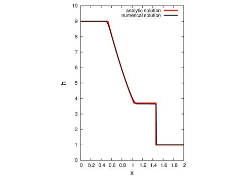
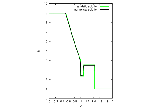
Figure 1: Comparison of the numerical and analytical solutions for the Riemann Problem. The surface is described by $z=1$; at the initial moment we have the velocity field $\boldsymbol{v}=\boldsymbol{0}$ and a discontinuity in the water-depth $h$: $\left\{h=9,\;{\rm for}\;x<1\right\}$, $\left\{h=1,\;{\rm for}\;x>1\right\}$. Left picture - constant porosity: $\theta=1$. Right picture - variable porosity: $\left\{\theta=0.8,\;{\rm for}\;x<1\right\}$, $\left\{\theta=1,\;{\rm for}\;x>1\right\}$.

Also, in Figure 2 we analyze the response of our model to the variation of the parameters.

6.2 External validation

Unfortunately, we do not have data for the water distribution, plant cover density and measured velocity field in a hydrographic basin to compare our numerical results with. However, to be closer to reality, we have used GIS data for the soil surface of Paul’s Valley and accomplished a theoretical experiment: starting with a uniform water depth on the entire basin and using different cover plant densities, we run our model, ASTERIX based on a hexagonal cellular automaton [10]. Figure 2 shows that the numerical results are consistent with direct observations concerning the water time residence in the hydrographic basin.

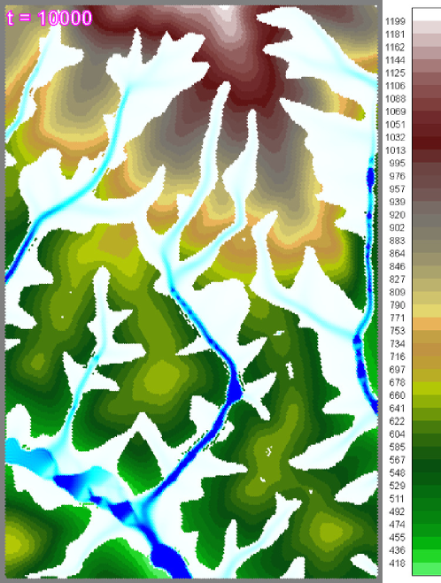
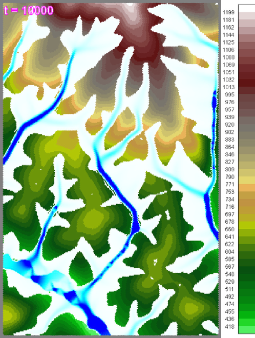
Figure 2: Snapshot of water distribution in Paul’s Valley hydrographic basin. Direct observations indicate that the water time residence depends on the density of the cover plant. Our numerical data are consistent with terrain observations: the water drainage time is bigger for the case of higher cover plant density. $\theta=3\%$ and $\theta=35\%$ for the left and right picture, respectively.

Figure 3 shows the results for the water content in Paul’s Valley basin obtained with our models ASTERIX and CAESAR-Lisflood-OSE [10, 9]. This variable $q$ is in fact the relative amount of water in the basin at the moment of time $t$:

$$q(t)=\displaystyle\frac{\displaystyle\int_{\Omega}h(t,x){\rm d}x}{\displaystyle\int_{\Omega}h(0,x){\rm d}x}.$$

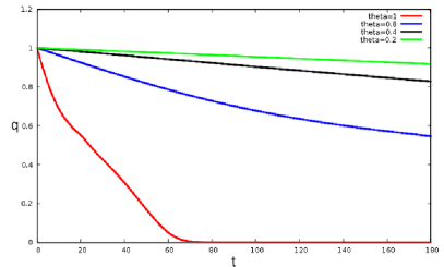
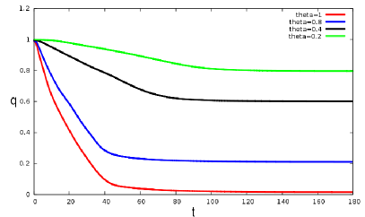
Figure 3: Time evolution of the water content in Paul’s Valley hydrographic basin with ASTERIX (left picture) and CAESAR (right picture).

This variable is also a measure of the amount of water leaving the basin. A general issue relates to whether higher cover plant densities can prevent soil erosion and flood or not. Both pictures show that if the cover plant density is increasing then the decreasing rate $\dot{q}$ of $q$ is smaller. We can think at a “characteristic velocity” of the water movement in the basin and this velocity is in a direct relation with $\dot{q}$. We can now speculate that smaller values of $\dot{q}$ imply softer erosion processes.

This valley belongs to Ampoi’s catchment basin. Flood generally appears when the discharge capacity of a river is overdue by the water coming from the river catchment area. Our pictures show that higher cover plant densities imply smaller values of $\dot{q}$ which in turn give Ampoi River the time to evacuate the water amount flowing from the valley.

References

• [1] M J Baptist, V Babovic, J Rodriguez Uthurburu, M Keijzer, R E Uittenbogaard, A Mynett, and A Verwey. On inducing equations for vegetation resistance. Journal of Hydraulic Research, 45(4):435–450, 2007.
• [2] F Bouchut. Nonlinear Stability of Finite Volume Methods for Hyperbolic Conservation Laws. Birkhäuser, Basel, 2004.
• [3] A Chinnayya, A Y LeRoux, and N Seguin. A well-balanced numerical scheme for the approximation of the shallow-water equations with topography: the resonance phenomenon. International Journal on Finite Volumes, 1:1–33, 2004.
• [4] TJ Coulthard, JC Neal, PD Bates, J Ramirez, GAM De Almeida, and GR Hancock. Integrating the LISFLOOD-FP 2d hydrodynamic model with the caesar model: implications for modelling landscape evolution. Earth Surface Processes and Landforms, 38:1897–1906, 2013.
• [5] J C I Dooge. A general theory of the unit hydrograph. Journal of Geophysical Research, 64(2):241–256, 1959.
• [6] U S Fjordholm, S Mishra, and E Tadmor. Well-balanced and energy stable schemes for the shallow water equations with discontinuous topography. Journal of Computational Physics, 230(14):5587–5609, 2011.
• [7] O Hájek. Discontinuous differential equations. Journal of Differential Equations, 32(2):149–170, 1979.
• [8] S Ion, D Marinescu, and S G Cruceanu. Overland flow in the presence of vegetation, 2013.
• [9] S Ion, D Marinescu, and S G Cruceanu. CAESAR-LISFLOOD-OSE, 2014.
• [10] S Ion, D Marinescu, S G Cruceanu, and V Iordache. A data porting tool for coupling models with different discretization needs. Environmental Modelling & Software, 62:240–252, 2014.
• [11] S Ion, D Marinescu, A-V Ion, S G Cruceanu, and V Iordache. Water flow on vegetated hill. 1d shalow water type equation type model. An. St. Univ. Ovidius, 23(3):83–96, 2015.
• [12] A Kurganov and G Petrova. A second-order well-balanced positivity preserving central-upwind scheme for the saint-venant system. Communications in Mathematical Sciences, 5(1):133–160, 2007.
• [13] R L LeVeque. Time-Split Methods for Partial Differential Equations. PhD thesis, Stanford University, Stanford, California, USA, 1982.
• [14] R L LeVeque. Finite Volume Methods for Hyperbolic Problems. Cambridge University Press, Cambridge, UK, 2002.
• [15] J J McDonnell, M Sivapalan, K Vachéand S Dunn, G Grant, R Haggerty, C Hinz, R Hooper, J Kirchner, M L Roderick, J Selker, and M Weiler. Moving beyond heterogeneity and process complexity: A new vision for watershed hydrology. Water Resources Research, 43(7):W07301, 1–6, 2007.
• [16] V Michel-Dansaca, C Berthon, S Clain, and F Foucher. A well-balanced scheme for the shallow-water equations with topography. Computers & Mathematics with Applications, 72(3):568–593, 2016.
• [17] H M Nepf. Drag, turbulence, and diffusion in flow through emergent vegetation. Water Resources Research, 35(2):479–489, 1999.
• [18] S Noelle, N Pankratz, G Puppo, and J R Natvig. Well-balanced finite volume schemes of arbitrary order of accuracy for shallow water flows. Journal of Computational Physics, 213(2):474–499, 2006.
• [19] K G Renard, G R Foster, G A Weesies, and J P Porter. Rusle: Revised universal soil loss equation. Journal of Soil and Water Conservation, 46(1):30–33, 1991.
• [20] G Strang. On the construction and comparison of difference schemes. SIAM Journal on Numerical Analysis, 5(3):506–517, 1968.
• [21] SWAP: Soil water atmosphere plant.
• [22] SWAT: Soil and water assessment tool.
• [23] W H Wischmeier. A rainfall erosion index for a universal soil-loss equation. Soil Science Society of America Journal, 23(3):246–249, 1959.
• [24] D A Woolhiser, R E Smith, and D C Goodrich. KINEROS: A kinematic runoff and erosion model: documentation and user manual. Technical report, ARS-77, U.S. Government, Washinton, D.C., USA, 1990.