Scattering of solutions to the defocusing energy sub-critical semi-linear wave equation in 3D

Abstract

In this paper we consider a semi-linear, energy sub-critical, defocusing wave equation $\partial_{t}^{2}u-\Delta u=-|u|^{p-1}u$ in the 3-dimensional space with $p\in[3,5)$. We prove that if initial data $(u_{0},u_{1})$ are radial so that $\|\nabla u_{0}\|_{L^{2}({\mathbb{R}}^{3};d\mu)},\|u_{1}\|_{L^{2}({\mathbb{R}}^{3};d\mu)}\leq\infty$, where $d\mu=(|x|+1)^{1+2\varepsilon}$ with $\varepsilon>0$, then the corresponding solution $u$ must exist for all time $t\in{\mathbb{R}}$ and scatter. The key ingredients of the proof include a transformation $\mathbf{T}$ so that $v=\mathbf{T}u$ solves the equation $v_{\tau\tau}-\Delta_{y}v=-\left(\frac{|y|}{\sinh|y|}\right)^{p-1}e^{-(p-3)\tau}|v|^{p-1}v$ with a finite energy, and a couple of global space-time integral estimates regarding a solution $v$ as above.

1 Introduction

The defocusing semi-linear wave equation

$$\left\{\begin{array}[]{ll}\partial_{t}^{2}u-\Delta u=-|u|^{p-1}u,&(x,t)\in{\mathbb{R}}^{3}\times{\mathbb{R}};\\ u(\cdot,0)=u_{0};&\\ u_{t}(\cdot,0)=u_{1}&\end{array}\right.\quad(CP1)$$

has been extensively studied in the past few decades. This problem is locally well-posed if initial data $(u_{0},u_{1})$ are contained in the critical Sobolev space $\dot{H}^{s_{p}}\times\dot{H}^{s_{p}-1}({\mathbb{R}}^{3})$ with $s_{p}\doteq 3/2-2/(p-1)$. Please see [14] for more details on the local theory. Suitable solutions also satisfy an energy conservation law:

$$E(u,u_{t})=\int_{{\mathbb{R}}^{3}}\left(\frac{1}{2}|\nabla u(\cdot,t)|^{2}+\frac{1}{2}|u_{t}(\cdot,t)|^{2}+\frac{1}{p+1}|u(\cdot,t)|^{p+1}\right)\,dx=\hbox{Const}.$$

The problem of global existence and scattering is much more difficult. In the energy critical case $p=5$, M. Grillakis [7] proved that any solution with initial data in the space $\dot{H}^{1}\times L^{2}({\mathbb{R}}^{3})$ must scatter in both two time directions. In other words, the asymptotic behaviour of any solution mentioned above resembles that of a free wave. It is conjectured that a similar result holds for other exponents $p$ as well: Any solution to (CP1) with initial data $(u_{0},u_{1})\in\dot{H}^{s_{p}}\times\dot{H}^{s_{p}-1}$ must exist for all time $t\in{\mathbb{R}}$ and scatter in both two time directions. This conjecture has not been proved yet, as far as the author knows, in spite of some progress:

• It has been proved that if a radial solution $u$ with a maximal lifespan $I$ satisfies an a priori estimate

  $$\sup_{t\in I}\left\|(u(\cdot,t),u_{t}(\cdot,t))\right\|_{\dot{H}^{s_{p}}\times\dot{H}^{s_{p}-1}({\mathbb{R}}^{3})}<+\infty,$$ (1)

  then $u$ is a global solution in time and scatters. The proof uses the standard compactness-rigidity argument, where the radial assumption plays a crucial role in the rigidity part. The details can be found in [12] for $p>5$, [15] for $3<p<5$ and [2] for $1+\sqrt{2}<p\leq 3$. The author would also like to mention that the same result still holds in the non-radial case if $p>5$, see [13]. Please note that our assumption (1) is automatically true in the energy critical case $p=5$, thanks to the conservation law of energy. When $p$ is other than $5$, however, nobody has ever found a way to actually prove this a priori estimate without additional assumptions on initial data.

• In the energy sub-critical case, the scattering result can be proved via conformal conservation laws if initial data satisfy an additional regularity-decay condition

  $$\int_{{\mathbb{R}}^{3}}\left[(|x|^{2}+1)(|\nabla u_{0}(x)|^{2}+|u_{1}(x)|^{2})+|u_{0}(x)|^{2}\right]dx<\infty.$$ (2)

  See [5, 8] for more details. Please pay attention that the radial assumption is not necessary in this argument.

Main Result

In this work we assume that initial data are still radial but satisfy a weaker decay condition than (2) and prove that the corresponding solution to (CP1) scatters. Let us first introduce our main theorem

Theorem 1.1.

Assume that $A,\varepsilon$ are positive constants and $3\leq p<5$. Let $(u_{0},u_{1})\in\dot{H}^{1}\times L^{2}$ be radial initial data so that

$$\|\nabla u_{0}\|_{L^{2}({\mathbb{R}}^{3};d\mu)},\|u_{1}\|_{L^{2}({\mathbb{R}}^{3};d\mu)}\leq A, d\mu=(|x|+1)^{1+2\varepsilon}dx.$$

Then the corresponding solution $u$ to (CP1) scatters in both two time directions with

$$\|u\|_{L^{2(p-1)}L^{2(p-1)}({\mathbb{R}}\times{\mathbb{R}}^{3})}\leq C(A,\varepsilon,p)<\infty.$$

Here the upper bound $C(A,\varepsilon,p)$ are solely determined by the values of $A$, $\varepsilon$ and $p$.

Here are some remarks regarding the initial data in the main theorem.

Remark 1.2.

The initial data $(u_{0},u_{1})$ satisfy the inequality

$$\int_{{\mathbb{R}}^{3}}\!\left(|\nabla u_{0}|^{\frac{3}{2}}+|u_{1}|^{\frac{3}{2}}\right)dx\leq 2\left[\int_{{\mathbb{R}}^{3}}\!\left(|\nabla u_{0}|^{2}+|u_{1}|^{2}\right)(1+|x|)^{1+2\varepsilon}\,dx\right]^{3/4}\left[\int_{{\mathbb{R}}^{3}}\!(1+|x|)^{-3-6\varepsilon}\,dx\right]^{1/4}$$

$$\leq C(A,\varepsilon)<\infty.$$

In other words we have $(u_{0},u_{1})\in\dot{W}^{1,3/2}\times L^{3/2}$. It immediately follows that $(u_{0},u_{1})\in\dot{H}^{s_{p}}\times\dot{H}^{s_{p}-1}$ by the Sobolev embedding $\dot{W}^{1,3/2}\times L^{3/2}\hookrightarrow\dot{H}^{1/2}\times\dot{H}^{-1/2}$ and an interpolation.

Remark 1.3.

The radial assumption implies that the initial data $(u_{0},u_{1})$ satisfy

$$\int_{0}^{\infty}\left(|\partial_{r}u_{0}(r)|^{2}+|u_{1}(r)|^{2}\right)r^{3+2\varepsilon}dr\leq(1/4\pi)A^{2}.$$

Remark 1.4.

Any pair $(u_{0},u_{1})$ as in Theorem 1.1 comes with a finite energy

$$E(u_{0},u_{1})=\int_{{\mathbb{R}}^{3}}\left[\frac{1}{2}|\nabla u_{0}(x)|^{2}+\frac{1}{2}|u_{1}(x)|^{2}+\frac{1}{p+1}|u_{0}(x)|^{p+1}\right]dx\leq C(A)<\infty.$$

In addition, $u_{0}$ satisfies a point-wise estimate $|u_{0}(x)|\leq A|x|^{-1-\varepsilon}$.

Proof.

By Remark 1.3 we have ($0<r_{1}<r_{2}<\infty$)

$$\left|u_{0}(r_{1})-u_{0}(r_{2})\right| \leq\int_{r_{1}}^{r_{2}}|\partial_{r}u_{0}(r)|dr\leq\left(\int_{r_{1}}^{r_{2}}|\partial_{r}u_{0}(r)|^{2}r^{3+2\varepsilon}dr\right)^{1/2}\left(\int_{r_{1}}^{r_{2}}r^{-3-2\varepsilon}dr\right)^{1/2}$$

$$\leq Ar_{1}^{-1-\varepsilon}.$$ (3)

Next we recall the point-wise estimate for radial $\dot{H}^{1}$ functions $|u_{0}(x)|\leq C\|u_{0}\|_{\dot{H}^{1}}|x|^{-1/2}$ as given in Lemma 3.2 of [12], make $r_{2}\rightarrow\infty$ in the inequality (3) above and obtain a point-wise estimate $|u_{0}(x)|\leq A|x|^{-1-\varepsilon}$. Furthermore, we can combine this point-wise estimate with the Sobolev embedding $\dot{H}^{1}({\mathbb{R}}^{3})\hookrightarrow L^{6}({\mathbb{R}}^{3})$ to conclude $\|u_{0}\|_{L^{p+1}({\mathbb{R}}^{3})}\leq C(A)$. This immediately gives a finite upper bound on the energy. ∎

The idea

In order to prove the main theorem, we need to show the following step by step.

• The solution $u$ is defined for all time $t\in{\mathbb{R}}$.

• The function $v=\mathbf{T}u$ defined by ($t_{0}$ is a time to be determined)

  $$v(y,\tau)=\frac{\sinh|y|}{|y|}e^{\tau}u\left(e^{\tau}\frac{\sinh|y|}{|y|}\cdot y,t_{0}+e^{\tau}\cosh|y|\right),\quad(y,\tau)\in{\mathbb{R}}^{3}\times{\mathbb{R}}$$

  solves the following non-linear wave equation with a finite energy

  $$v_{\tau\tau}-\Delta_{y}v=-\left(\frac{|y|}{\sinh|y|}\right)^{p-1}e^{-(p-3)\tau}|v|^{p-1}v.\quad(\hbox{CP2})$$

• The solution $v$ satisfies a few space-time integral estimates.

• We rewrite the information about $v$ obtained in the previous step in term of $u$ and finally conclude $\|u\|_{L^{2(p-1)}L^{2(p-1)}({\mathbb{R}}\times{\mathbb{R}}^{3})}<\infty$. This is equivalent to the scattering of $u$, as shown in Subsection 3.4.

The transformation from $u$ to $v$ above is one of the key ingredients of our proof. Its validity can be verified by a basic calculation, as given in Section 5. The author would also like to mention that the transformation can be constructed via two different routes:

Route 1

We can write $\mathbf{T}=\mathbf{T}_{2}\circ\mathbf{T}_{1}$. Here $\mathbf{T}_{1}$ is a transformation from the set of functions defined on the forward light cone $\{(x,t):t-t_{0}>|x|\}$ to the set of functions defined on ${\mathbb{H}}^{3}\times{\mathbb{R}}$, whose formula has been given by D. Tataru in the work [18]:

$$(\mathbf{T}_{1}u)(s,\Theta,\tau)=e^{\tau}u(e^{\tau}\sinh s\cdot\Theta,t_{0}+e^{\tau}\cosh s).$$

Here $(s,\Theta)\in[0,\infty)\times{\mathbb{S}}^{2}$ are polar coordinates on the hyperbolic space ${\mathbb{H}}^{3}$. One can demonstrate the importance of this transformation by the fact

$$(\partial_{\tau}^{2}-\Delta_{{\mathbb{H}}^{3}}-1)\circ\mathbf{T}_{1}=e^{2\tau}\mathbf{T}_{1}\circ(\partial_{t}^{2}-\Delta).$$

As a result, if $u$ is a solution to (CP1), then the function $v_{1}=\mathbf{T}_{1}u$ solves the non-linear shifted wave equation on ${\mathbb{H}}^{3}$ (See [1, 16, 17] for Strichartz estimates and local theory on this type of equations)

$$\partial_{\tau}^{2}v_{1}-(\Delta_{{\mathbb{H}}^{3}}+1)v_{1}=-e^{-(p-3)\tau}|v_{1}|^{p-1}v_{1}.$$ (4)

Next we introduce the second transformation $(\mathbf{T}_{2}v_{1})(y,\tau)=\frac{\sinh|y|}{|y|}v_{1}(|y|,\tau)$, whose domain is the set of radial functions on ${\mathbb{H}}^{3}\times{\mathbb{R}}$ and whose range is the set of radial functions on ${\mathbb{R}}^{3}\times{\mathbb{R}}$. This transformation satisfies $(\partial_{\tau}^{2}-\Delta_{y})\circ\mathbf{T}_{2}=\mathbf{T}_{2}\circ(\partial_{\tau}^{2}-\Delta_{{\mathbb{H}}^{3}}-1)$. A basic calculation shows that if $v_{1}$ solves (4), then $v=\mathbf{T}_{2}v_{1}$ satisfies (CP2).

Route 2

We have another decomposition $\mathbf{T}=\mathbf{T}_{3}^{-1}\circ\mathbf{T}_{4}\circ\mathbf{T}_{3}$, where

$$(\mathbf{T}_{3}u)(|x|,t)=|x|u(x,t); (\mathbf{T}_{4}w)(s,\tau)=w(e^{\tau}\sinh s,t_{0}+e^{\tau}\cosh s).$$

Both $\mathbf{T}_{3}u$ and $\mathbf{T}_{4}w$ are functions defined on $[0,\infty)\times{\mathbb{R}}$. These two transformations satisfy the commutator identities

$$(\partial_{t}^{2}-\partial_{r}^{2})\circ\mathbf{T}_{3}=\mathbf{T}_{3}\circ(\partial_{t}^{2}-\Delta_{x}); (\partial_{\tau}^{2}-\partial_{s}^{2})\circ\mathbf{T}_{4}=e^{2\tau}\mathbf{T}_{4}\circ(\partial_{t}^{2}-\partial_{r}^{2}).$$

As a result, if $u$ is a radial solution to (CP1), then $w=\mathbf{T}_{3}u$ and $w_{1}=\mathbf{T}_{4}w$ solve the non-linear wave equations $\partial_{t}^{2}w-\partial_{r}^{2}w=-\frac{1}{r^{p-1}}|w|^{p-1}w$ and $\partial_{\tau}^{2}w_{1}-\partial_{s}^{2}w_{1}=-e^{-(p-3)\tau}\frac{1}{\sinh^{p-1}s}|w_{1}|^{p-1}w_{1}$, respectively.

The structure of this paper

This paper is organized as follows. In section 2 we collect notations, recall the Strichartz estimates and introduce a local theory for a class of wave equations in the form of $\partial_{t}^{2}u-\Delta u=-\phi(x)e^{-\kappa t}|u|^{p-1}u$ with a function $\phi:{\mathbb{R}}^{3}\rightarrow[-1,1]$ and a constant $\kappa\geq 0$. In particular, we combine the energy conservation law with our local theory to conclude that any solution to (CP1) with a finite energy is defined for all time. Next in Section 3 we discuss the global behaviour of solutions to the wave equation above with a suitable coefficient function $\phi(x)$. More precisely, we prove a few global space-time integral estimates if the initial data come with a finite energy, one of which is a Morawetz-type estimate. After all of these preparation work is finished, we prove the main theorem in the last three sections. In Section 4 we start by proving a few preliminary estimates on the solutions $u$ to (CP1). Then we apply the transformation $\mathbf{T}$ and show that $v=\mathbf{T}u$ is indeed a solution to (CP2) in Section 5. In the final section we verify that $v$ has a finite energy, take advantage of the space-time integral estimates we obtained in Section 3, rewrite them in term of $u$ and eventually finish the proof.

2 Preliminary Results

2.1 Notations

The $\lesssim$ symbol

We use the notation $A\lesssim B$ if there exists a constant $c$, so that the inequality $A\leq cB$ always holds. In addition, a subscript of the symbol $\lesssim$ indicates that the constant $c$ is determined by the parameter(s) mentioned in the subscript but nothing else. In particular, $\lesssim_{1}$ means that the constant $c$ is an absolute constant.

Radial functions

Let $u(x,t)$ be a spatially radial function. By convention $u(r,t)$ represents the value of $u(x,t)$ when $|x|=r$.

Linear wave propagation

Given a pair of initial data $(u_{0},u_{1})$, we define $\mathbf{S}_{L,0}(t)(u_{0},u_{1})$ to be the solution $u$ of the free linear wave equation $u_{tt}-\Delta u=0$ with initial data $(u,u_{t})|_{t=0}=(u_{0},u_{1})$. If we are also interested in the velocity $u_{t}$, we can use the notation

$$\mathbf{S}_{L}(t)(u_{0},u_{1})\doteq(u(\cdot,t),u_{t}(\cdot,t)), \mathbf{S}_{L}(t)\begin{pmatrix}u_{0}\\ u_{1}\end{pmatrix}\doteq\begin{pmatrix}u(\cdot,t)\\ u_{t}(\cdot,t)\end{pmatrix}.$$

2.2 Local theory

In this subsection we consider the local theory of the equation

$$\left\{\begin{array}[]{ll}\partial_{t}^{2}v-\Delta v=-\phi(x)e^{-\kappa t}|v|^{p-1}v,&(x,t)\in{\mathbb{R}}^{3}\times{\mathbb{R}};\\ v(\cdot,t_{0})=v_{0}\in\dot{H}^{1}({\mathbb{R}}^{3});&\\ v_{t}(\cdot,t_{0})=v_{1}\in L^{2}({\mathbb{R}}^{3}).&\end{array}\right.$$ (5)

Here $\phi:{\mathbb{R}}^{3}\rightarrow[-1,1]$ is a measurable function, $\kappa$ is a nonnegative constant and $p\in[3,5)$. This covers both equations (CP1) and (CP2).

Definition 2.1.

We say that a solution $v$ solves the equation (5) in a time interval $I$ containing $t_{0}$, if $v$ satisfies

• $(v(\cdot,t),v_{t}(\cdot,t))\in C(I;\dot{H}^{1}\times L^{2}({\mathbb{R}}^{3}))$;

• The norm $\|v\|_{L^{2p/(p-3)}L^{2p}(J\times{\mathbb{R}}^{3})}$ is finite for any bound closed interval $J\subseteq I$;

• The integral equation

  $$v(\cdot,t)=\mathbf{S}_{L,0}(t-t_{0})(v_{0},v_{1})+\int_{t_{0}}^{t}\frac{\sin((t-\tau)\sqrt{-\Delta})}{\sqrt{-\Delta}}G(\cdot,\tau,v(\cdot,\tau))d\tau$$

  holds for all $t\in I$, here $G(x,t,v)=-\phi(x)e^{-\kappa t}|v|^{p-1}v$.

Strichartz estimates

The basis of our local theory is the following generalized Strichartz estimates. (Please see Proposition 3.1 of [6], here we use the Sobolev version in ${\mathbb{R}}^{3}$)

Proposition 2.2.

Let $2\leq q_{1},q_{2}\leq\infty$, $2\leq r_{1},r_{2}<\infty$ and $\rho_{1},\rho_{2},s\in{\mathbb{R}}$ with

$$1/{q_{i}}+1/{r_{i}}\leq 1/2,\quad i=1,2;$$

$$1/{q_{1}}+3/{r_{1}}=3/2-s^{\prime}+\rho_{1}; 1/{q_{2}}+3/{r_{2}}=1/2+s^{\prime}+\rho_{2}.$$

Let $v$ be the solution of the following linear wave equation ($t_{0}\in I$)

$$\left\{\begin{array}[]{ll}\partial_{t}^{2}v-\Delta v=F(x,t),&(x,t)\in{\mathbb{R}}^{3}\times I;\\ (v,v_{t})|_{t=t_{0}}=(v_{0},v_{1})\in\dot{H}^{s^{\prime}}({\mathbb{R}}^{3})\times\dot{H}^{s^{\prime}-1}({\mathbb{R}}^{3}).\end{array}\right.$$ (6)

Then there exists a constant independent of $I$ and initial data $(u_{0},u_{1})$, so that

$$\|(v(\cdot,t),v_{t}(\cdot,t))\|_{C(I;\dot{H}^{s^{\prime}}\times\dot{H}^{s^{\prime}-1})}+\|D_{x}^{\rho_{1}}v\|_{L^{q_{1}}L^{r_{1}}(I\times{\mathbb{R}}^{3})}$$

$$\qquad\leq C\left(\|(v_{0},v_{1})\|_{\dot{H}^{s^{\prime}}\times\dot{H}^{s^{\prime}-1}}+\|D_{x}^{-\rho_{2}}F(x,t)\|_{L^{\bar{q}_{2}}L^{\bar{r}_{2}}(I\times{\mathbb{R}}^{3})}\right).$$

A fixed-point argument

We first choose specific coefficients $\rho_{1}=\rho_{2}=0$, $s^{\prime}=1$, $(q_{1},r_{1})=(2p/(p-3),2p)$, $(q_{2},r_{2})=(\infty,2)$ in the Strichartz estimates

$$\left\|(v(\cdot,t),v_{t}(\cdot,t))\right\|_{C([t_{1},t_{2}];\dot{H}^{1}\times L^{2})}+\|v\|_{L^{\frac{2p}{p-3}}L^{2p}([t_{1},t_{2}]\times{\mathbb{R}}^{3})}$$

$$\qquad\quad\leq C_{p}\left[\|(v(\cdot,t_{1}),v_{t}(\cdot,t_{1}))\|_{\dot{H}^{1}\times L^{2}}+\|(\partial_{t}^{2}-\Delta)v\|_{L^{1}L^{2}([t_{1},t_{2}]\times{\mathbb{R}}^{3})}\right],$$

and observe the inequalities

$$\|G(\cdot,\cdot,v)\|_{L^{1}L^{2}([t_{1},t_{2}]\times{\mathbb{R}}^{3})} \leq e^{-\kappa t_{1}}(t_{2}-t_{1})^{\frac{5-p}{2}}\|v\|_{L^{\frac{2p}{p-3}}L^{2p}([t_{1},t_{2}]\times{\mathbb{R}}^{3})}^{p};$$

$$\|G(\cdot,\cdot,v_{1})-G(\cdot,\cdot,v_{2})\|_{L^{1}L^{2}([t_{1},t_{2}]\times{\mathbb{R}}^{3})} \leq\left[\|v_{1}\|_{L^{\frac{2p}{p-3}}L^{2p}([t_{1},t_{2}]\times{\mathbb{R}}^{3})}^{p-1}+\|v_{2}\|_{L^{\frac{2p}{p-3}}L^{2p}([t_{1},t_{2}]\times{\mathbb{R}}^{3})}^{p-1}\right]$$

$$\qquad\times e^{-\kappa t_{1}}(t_{2}-t_{1})^{\frac{5-p}{2}}\|v_{1}-v_{2}\|_{L^{\frac{2p}{p-3}}L^{2p}([t_{1},t_{2}]\times{\mathbb{R}}^{3})}.$$

A fixed-point argument then shows (Our argument is similar to a lot of earlier works. See [9, 14], for instance.)

Theorem 2.3 (Local solution).

Given a time $t_{0}$ and a pair $(v_{0},v_{1})\in\dot{H}^{1}\times L^{2}$, then there is a maximal time interval $(t_{0}-T_{-}(v_{0},v_{1},t_{0}),t_{0}+T_{+}(v_{0},v_{1},t_{0}))$ in which the equation (5) with the initial condition $(v,v_{t})|_{t=t_{0}}=(v_{0},v_{1})$ has a unique solution $v(x,t)$. In addition we have

$$T_{+}(v_{0},v_{1},t_{0})>T_{1} \doteq C_{1}(p)e^{2\kappa t_{0}/(5-p)}\|(v_{0},v_{1})\|_{\dot{H}^{1}\times L^{2}({\mathbb{R}}^{3})}^{-2(p-1)/(5-p)};$$

$$\|v(x,t)\|_{L^{2p/(p-3)}L^{2p}([t_{0},t_{0}+T_{1}]\times{\mathbb{R}}^{3})} \leq C_{2}(p)\|(v_{0},v_{1})\|_{\dot{H}^{1}\times L^{2}({\mathbb{R}}^{3})}.$$

Remark 2.4.

If $v$ is a solution to (5), then we have $\|D^{1/2}v\|_{L^{4}L^{4}([a,b]\times{\mathbb{R}}^{3})}<+\infty$ for any finite bounded interval $[a,b]$ contained in the maximal lifespan of $v$ by the Strichartz estimates.

Proposition 2.5.

Any solution $u$ to (CP1) is global in time, i.e. it has a maximal lifespan ${\mathbb{R}}$.

Proof.

The conservation law of energy guarantees that the norm $\|(u(\cdot,t),u_{t}(\cdot,t))\|_{\dot{H}^{1}\times L^{2}}\lesssim E^{1/2}$ is uniformly bounded for all time $t$ in the maximal lifespan of $u$. The combination of this fact and Theorem 2.3 implies that $u$ is well-defined for all $t>0$. Since (CP1) is time-invertible, we are able to conclude that the maximal lifespan of $u$ must be ${\mathbb{R}}$. ∎

Perturbation theory

Next let us consider the continuous dependence of the solutions to (5) on the initial data. The special case with $\phi(x)\equiv 1$ and $\kappa=0$ has been proved in Appendix of [15]. We can prove the general case in exactly the same way.

Theorem 2.6.

Let $\tilde{v}$ be a solution of equation (5) in a bounded time interval $I$ with initial data $(\tilde{v}_{0},\tilde{v}_{1})$, so that

$$\|(\tilde{v}_{0},\tilde{v}_{1})\|_{\dot{H}^{1}\times L^{2}}<\infty; \|\tilde{v}\|_{L^{2p/(p-3)}L^{2p}(I\times{\mathbb{R}}^{3})}<M.$$

There exist two constants $\varepsilon_{0}(I,M),C(I,M)>0$, such that if $(v_{0},v_{1})\in\dot{H}^{1}\times L^{2}$ satisfy

$$\|(v_{0}-\tilde{v}_{0},v_{1}-\tilde{v}_{1})\|_{\dot{H}^{1}\times L^{2}}<\varepsilon_{0}(I,M),$$

then the corresponding solution $v$ of (5) with initial data $(v_{0},v_{1})$ is well-defined in $I$ so that

$$\|v-\tilde{v}\|_{L^{2p/(p-3)}L^{2p}(I\times{\mathbb{R}}^{3})} \leq C(I,M)\|(v_{0}-\tilde{v}_{0},v_{1}-\tilde{v}_{1})\|_{\dot{H}^{1}\times L^{2}};$$

$$\left\|\begin{pmatrix}v(\cdot,t)\\ v_{t}(\cdot,t)\end{pmatrix}-\begin{pmatrix}\tilde{v}(\cdot,t)\\ \tilde{v}_{t}(\cdot,t)\end{pmatrix}\right\|_{C(I;\dot{H}^{1}\times L^{2})} \leq C(I,M)\|(v_{0}-\tilde{v}_{0},v_{1}-\tilde{v}_{1})\|_{\dot{H}^{1}\times L^{2}}.$$

3 A Wave Equation with a Time Dependent Nonlinearity

In this section we discuss the global behaviour of the solutions to the equation

$$\left\{\begin{array}[]{ll}v_{tt}-\Delta u=-\phi(x)e^{-\kappa t}|v|^{p-1}v,&(x,t)\in{\mathbb{R}}^{3}\times{\mathbb{R}};\\ v(\cdot,t_{0})=v_{0}\in\dot{H}^{1}({\mathbb{R}}^{3})\cap L^{p+1}({\mathbb{R}}^{3};\phi(x)dx);&\\ v_{t}(\cdot,t_{0})=v_{1}\in L^{2}({\mathbb{R}}^{3}).&\end{array}\right.$$ (7)

Here we assume that $p\in[3,5)$, $\kappa\geq 0$ are constants and $\phi:{\mathbb{R}}^{3}\rightarrow[0,1]$ is a measurable function. The equation (CP2) corresponds to the case with $\kappa=p-3$ and $\phi(x)=\left(\frac{|x|}{\sinh|x|}\right)^{p-1}$. In this case the parameter $\kappa>0$ whenever $p>3$.

3.1 Monotonicity of the Energy

Now let us consider the “energy” defined by

$$E(t)=\int_{{\mathbb{R}}^{3}}\left[\frac{1}{2}|\nabla_{x}v(x,t)|^{2}+\frac{1}{2}|v_{t}(x,t)|^{2}+e^{-\kappa t}\phi(x)\frac{|v(x,t)|^{p+1}}{p+1}\right]dx.$$

If $u$ is sufficiently smooth and decays sufficiently fast near infinity, we can differentiate and obtain

$$E^{\prime}(t)= \int_{{\mathbb{R}}^{3}}\left[\nabla v\nabla v_{t}+v_{t}v_{tt}+e^{-\kappa t}\phi(x)|v|^{p-1}vv_{t}-\kappa e^{-\kappa t}\phi\frac{|v|^{p+1}}{p+1}\right]dx$$

$$= \int_{{\mathbb{R}}^{3}}v_{t}\left(-\Delta v+v_{tt}+e^{-\kappa t}\phi|v|^{p-1}v\right)dx-\frac{\kappa}{p+1}\int_{{\mathbb{R}}^{3}}e^{-\kappa t}\phi|v|^{p+1}dx$$

$$= -\frac{\kappa}{p+1}\int_{{\mathbb{R}}^{3}}e^{-\kappa t}\phi(x)|v(x,t)|^{p+1}dx\leq 0.$$

One can verify that this formula of $E^{\prime}(t)$ works for general solutions $v$ of the Cauchy problem (7) as well by standard smooth approximation and cut-off techniques. Therefore we have

Proposition 3.1.

Let $v$ be a solution to the Cauchy problem (7) in a time interval $[t_{0},t_{0}+T_{+})$ with $E(t_{0})<\infty$.

• If $\kappa>0$, then $E(t)$ is a non-increasing function of $t\in[t_{0},t_{0}+T_{+})$. In addition, we have the integral estimate

  $$\int_{t_{0}}^{t_{0}+T_{+}}\!\!\int_{{\mathbb{R}}^{3}}e^{-\kappa t}\phi(x)|v(x,t)|^{p+1}dx\,dt\leq\frac{p+1}{\kappa}E(t_{0}).$$

• If $\kappa=0$, then $E(t)$ is a constant independent of $t$.

3.2 Global behaviour in the positive time direction

Assume that $v$ is a solution to the Cauchy problem (7) with a maximal lifespan $(t_{0}-T_{-},t_{0}+T_{+})$. Given any $t\in I_{+}\doteq[t_{0},t_{0}+T_{+})$, Proposition 3.1 implies

$$\|(v(\cdot,t),v_{t}(\cdot,t))\|_{\dot{H}^{1}\times L^{2}}\leq\left[2E(t)\right]^{1/2}\leq\left[2E(t_{0})\right]^{1/2}.$$

According to Theorem 2.3, this means that there are two positive constants $T_{1}$ and $N_{1}$, such that if $t\in I_{+}$, then we have $[t,t+T_{1}]\subseteq I_{+}$ and $\|v\|_{L^{2p/(p-3)}L^{2p}([t,t+T_{1}])}\leq N_{1}$. It immediately follows that $T_{+}=+\infty$. Namely the solution $u$ is defined for all time $t>t_{0}$. Furthermore, if $\kappa>0$ we have

$$\left\|G(x,t,v)\right\|_{L_{t}^{1}L_{x}^{2}([t_{0},\infty)\times{\mathbb{R}}^{3})}= \sum_{j=0}^{\infty}\left\|e^{-\kappa t}\phi(x)|v|^{p-1}v\right\|_{L^{1}L^{2}([t_{0}+jT_{1},t_{0}+(j+1)T_{1}]\times{\mathbb{R}}^{3})}$$

$$= \sum_{j=0}^{\infty}e^{-\kappa t_{0}-j\kappa T_{1}}T_{1}^{(5-p)/2}\|v\|_{L^{2p/(p-3)}L^{2p}([t_{0}+jT_{1},t_{0}+(j+1)T_{1}]\times{\mathbb{R}}^{3})}^{p}$$

$$= \sum_{j=0}^{\infty}e^{-\kappa t_{0}-j\kappa T_{1}}T_{1}^{(5-p)/2}N_{1}^{p}<\infty.$$

Recalling the Strichartz estimates and the fact that the linear wave propagation preserves the $\dot{H}^{1}\times L^{2}$ norm, we obtain

$$\lim_{t_{1},t_{2}\rightarrow+\infty}\left\|\mathbf{S}_{L}(-t_{1})\begin{pmatrix}v(\cdot,t_{1})\\ v_{t}(\cdot,t_{1})\end{pmatrix}-\mathbf{S}_{L}(-t_{2})\begin{pmatrix}v(\cdot,t_{2})\\ v_{t}(\cdot,t_{2}))\end{pmatrix}\right\|_{\dot{H}^{1}\times L^{2}}$$

$$= \lim_{t_{1},t_{2}\rightarrow+\infty}\left\|\mathbf{S}_{L}(t_{2}-t_{1})\begin{pmatrix}v(\cdot,t_{1})\\ v_{t}(\cdot,t_{1})\end{pmatrix}-\begin{pmatrix}v(\cdot,t_{2})\\ v_{t}(\cdot,t_{2}))\end{pmatrix}\right\|_{\dot{H}^{1}\times L^{2}}$$

$$\leq \lim_{t_{1},t_{2}\rightarrow+\infty}\|G(x,t,v)\|_{L_{t}^{1}L_{x}^{2}([t_{1},t_{2}]\times{\mathbb{R}}^{3})}=0.$$

As a result, the pair $\mathbf{S}_{L}(-t)(v(\cdot,t),v_{t}(\cdot,t))$ converges in the space $\dot{H}^{1}\times L^{2}$ as $t\rightarrow\infty$. Let us assume $\mathbf{S}_{L}(-t)(v(\cdot,t),v_{t}(\cdot,t))\rightarrow(v_{0}^{+},v_{1}^{+})$. This is equivalent to saying

$$\lim_{t\rightarrow+\infty}\left\|(v(\cdot,t),v_{t}(\cdot,t))-\mathbf{S}_{L}(t)(v_{0}^{+},v_{1}^{+})\right\|_{\dot{H}^{1}\times L^{2}}=0.$$

We summarize our results below

Theorem 3.2 (Global behaviour).

Let $v$ be a solution to the Cauchy problem (7) with a finite energy $E(t_{0})<\infty$. Then $v$ is well-defined for all $t\geq t_{0}$. If we also have $\kappa>0$, then there exists a pair $(v_{0}^{+},v_{1}^{+})\in\dot{H}^{1}\times L^{2}$ so that

$$\lim_{t\rightarrow\infty}\left\|(v(\cdot,t),v_{t}(\cdot,t))-\mathbf{S}_{L}(t)(v_{0}^{+},v_{1}^{+})\right\|_{\dot{H}^{1}\times L^{2}}=0.$$

A combination of Theorem 3.2 and Proposition 3.1 immediately gives

Corollary 3.3.

Let $v$ be a solution to the Cauchy problem (7) with $\kappa>0$ and a finite energy $E(t_{0})<\infty$. Then we have

$$\int_{t_{0}}^{\infty}\int_{{\mathbb{R}}^{3}}e^{-\kappa t}\phi(x)|v(x,t)|^{p+1}dx\,dt\leq\frac{p+1}{\kappa}E(t_{0}).$$

3.3 A Morawetz-type Inequality

Proposition 3.4.

Let $v$ be a solution to the Cauchy problem (7) in a time interval $[t_{0},t_{0}+T_{+})$ so that

• $E(t_{0})<\infty$;

• The inequalities $0\leq\phi(x)\leq 1$ and $(p-1)\phi-x\cdot\nabla\phi\geq 0$ hold for all $x\in{\mathbb{R}}^{3}$.

Then we have the following Morawetz-type inequality

$$\int_{t_{0}}^{t_{0}+T_{+}}\!\!\int_{{\mathbb{R}}^{3}}e^{-\kappa t}\cdot\frac{(p-1)\phi-x\cdot\nabla\phi}{|x|}\cdot|v|^{p+1}dx\,dt\lesssim_{1}E(t_{0}).$$

Outline of the proof

Let us consider a function $a(x)=|x|$ and define

$$M(t)=\int_{{\mathbb{R}}^{3}}v_{t}(x,t)\left(\nabla v(x,t)\cdot\nabla a(x)+\frac{1}{2}\Delta a(x)v(x,t)\right)dx.$$

A basic calculation shows

$$\nabla a=\frac{x}{|x|}, \Delta a=\frac{2}{|x|}, \mathbf{D}^{2}a\geq 0, \Delta\Delta a\leq 0.$$

As a result, we obtain an upper bound on $|M(t)|$ by Hardy’s inequality $\|v/|x|\|_{L^{2}}\lesssim\|\nabla v\|_{L^{2}}$:

$$\left|M(t)\right|\leq\|v_{t}(\cdot,t)\|_{L^{2}}\left(\|\nabla v(\cdot,t)\|_{L^{2}}+\|v(x,t)/|x|\|_{L_{x}^{2}({\mathbb{R}}^{3})}\right)\lesssim_{1}E(t).$$ (8)

Next we calculate the derivative $M^{\prime}(t)$ informally

$$M^{\prime}(t)= \int_{{\mathbb{R}}^{3}}v_{tt}\left(\nabla v\cdot\nabla a+\frac{1}{2}v\Delta a\right)dx+\int_{{\mathbb{R}}^{3}}v_{t}\left(\nabla v_{t}\cdot\nabla a+\frac{1}{2}v_{t}\Delta a\right)dx$$

$$= \int_{{\mathbb{R}}^{3}}\Delta v\left(\nabla v\cdot\nabla a+\frac{1}{2}v\Delta a\right)dx-\int_{{\mathbb{R}}^{3}}\phi(x)e^{-\kappa t}|v|^{p-1}v\left(\nabla v\cdot\nabla a+\frac{1}{2}v\Delta a\right)dx$$

$$\qquad+\int_{{\mathbb{R}}^{3}}v_{t}\left(\nabla v_{t}\cdot\nabla a+\frac{1}{2}v_{t}\Delta a\right)dx$$

$$= I_{1}+I_{2}+I_{3}.$$

Let us start with $I_{1}$. For simplicity we use lower indices to represent partial derivatives.

$$I_{1}= \int_{{\mathbb{R}}^{3}}\left(\sum_{i,j=1}^{3}v_{ii}v_{j}a_{j}\right)dx-\frac{1}{2}\int_{{\mathbb{R}}^{3}}|\nabla v|^{2}\Delta a\,dx-\frac{1}{2}\int_{{\mathbb{R}}^{3}}v\nabla v\cdot\nabla\Delta a\,dx$$

$$= -\int_{{\mathbb{R}}^{3}}\left(\sum_{i,j=1}^{3}a_{ij}v_{i}v_{j}\right)dx-\int_{{\mathbb{R}}^{3}}\left(\sum_{i,j=1}^{3}a_{j}v_{i}v_{ij}\right)dx-\frac{1}{2}\int_{{\mathbb{R}}^{3}}|\nabla v|^{2}\Delta a\,dx+\frac{1}{4}\int_{{\mathbb{R}}^{3}}|v|^{2}\Delta\Delta a\,dx$$

$$\leq -\frac{1}{2}\int_{{\mathbb{R}}^{3}}\nabla a\cdot\nabla(|\nabla v|^{2})dx-\frac{1}{2}\int_{{\mathbb{R}}^{3}}|\nabla v|^{2}\Delta a\,dx$$

$$= 0.$$

Here we use the facts $\mathbf{D}^{2}a\geq 0$ and $\Delta\Delta a\leq 0$. In addition we have

$$I_{2}= -\frac{1}{p+1}\int_{{\mathbb{R}}^{3}}\phi(x)e^{-\kappa t}\nabla(|v|^{p+1})\cdot\nabla a\,dx-\frac{1}{2}\int_{{\mathbb{R}}^{3}}\phi(x)e^{-\kappa t}|v|^{p+1}\Delta a\,dx$$

$$= \frac{1}{p+1}\int_{{\mathbb{R}}^{3}}e^{-\kappa t}|v|^{p+1}\nabla\phi\cdot\nabla adx+\left(\frac{1}{p+1}-\frac{1}{2}\right)\int_{{\mathbb{R}}^{3}}e^{-\kappa t}|v|^{p+1}\phi\Delta a\,dx$$

$$= \frac{1}{p+1}\int_{{\mathbb{R}}^{3}}e^{-\kappa t}|v|^{p+1}\left(\nabla\phi\cdot\nabla a-\frac{p-1}{2}\phi\Delta a\right)dx$$

$$= \frac{-1}{p+1}\int_{t_{1}}^{t_{2}}\!\!\int_{{\mathbb{R}}^{3}}e^{-\kappa t}\cdot\frac{(p-1)\phi-x\cdot\nabla\phi}{|x|}\cdot|v|^{p+1}dx\,dt.$$

Finally

$$I_{3}=\frac{1}{2}\int_{{\mathbb{R}}^{3}}\nabla(|\partial_{t}v|^{2})\cdot\nabla a\,dx+\frac{1}{2}\int_{{\mathbb{R}}^{3}}|\partial_{t}v|^{2}\Delta a\,dx=0.$$

Now we collect all the terms above and then integrate from $t=t_{1}$ to $t=t_{2}$:

$$M(t_{2})-M(t_{1})\leq \frac{-1}{p+1}\int_{t_{1}}^{t_{2}}\!\!\int_{{\mathbb{R}}^{3}}e^{-\kappa t}\cdot\frac{(p-1)\phi-x\cdot\nabla\phi}{|x|}\cdot|v|^{p+1}dx\,dt.$$

We plug the upper bound on $|M(t)|$ as given in (8) into the left hand side above, recall the monotonicity of $E(t)$ and finally complete our proof.

Remark 3.5.

The argument above works only for solutions $v$ that satisfies certain regularity conditions. However, Proposition 3.4 still holds for all solutions $v$ with a finite energy $E(t_{0})<\infty$. This can be proved via standard smooth approximation and cut-off techniques. Please refer to Section 4 of [16] for more details about this type of argument.

3.4 An Equivalent Condition of Scattering

Let us start by a technical result.

Proposition 3.6.

Let $v$ be a solution to the Cauchy problem (7) in a bounded closed time interval $I=[a,b]$ with initial data $(v_{0},v_{1})\in(\dot{H}^{1}\cap\dot{H}^{s_{p}})\times(L^{2}\cap\dot{H}^{s_{p}-1})$. Then we have $(v(\cdot,t),v_{t}(\cdot,t))\in C(I;\dot{H}^{s_{p}}\times\dot{H}^{s_{p}-1})$ and

$$\|D^{s_{p}-1/2}v\|_{L^{4}L^{4}([a,b]\times{\mathbb{R}}^{3})}<+\infty.$$

Proof.

Let us recall the Strichartz estimate

$$\|(v(\cdot,t),v_{t}(\cdot,t))\|_{C(I;\dot{H}^{s_{p}}\times\dot{H}^{s_{p}-1})} +\|D^{s_{p}-1/2}v\|_{L^{4}L^{4}([a,b]\times{\mathbb{R}}^{3})}$$

$$\lesssim\|(v_{0},v_{1})\|_{\dot{H}^{s_{p}}\times\dot{H}^{s_{p}-1}}+\|(\partial_{t}^{2}-\Delta)v\|_{L^{\frac{2}{1+s_{p}}}L^{\frac{2}{2-s_{p}}}(I\times{\mathbb{R}}^{3})}.$$

As a result, it suffices to show

$$\left\|-e^{-\kappa t}\phi(x)|v|^{p-1}v\right\|_{L^{\frac{2}{1+s_{p}}}L^{\frac{2}{2-s_{p}}}(I\times{\mathbb{R}}^{3})}<\infty\Leftrightarrow\left\|\phi^{1/p}v\right\|_{L^{\frac{4(p-1)p}{5p-9}}L^{\frac{4(p-1)p}{p+3}}(I\times{\mathbb{R}}^{3})}<\infty.$$ (9)

On one hand, the monotonicity of $E(t)$ implies

$$\sup_{t\in I}\int_{{\mathbb{R}}^{3}}e^{-\kappa t}\phi(x)|v(x,t)|^{p+1}dx\,dt<\infty\Rightarrow\left\|\phi^{1/p}v\right\|_{L^{\infty}L^{p+1}(I\times{\mathbb{R}}^{3})}<\infty.$$

On the other hand, the Strichartz estimates give

$$\|v\|_{L^{5}L^{10}(I\times{\mathbb{R}}^{3})}<\infty\Longrightarrow\left\|\phi^{1/p}v\right\|_{L^{5}L^{10}(I\times{\mathbb{R}}^{3})}<\infty.$$

We combine these two inequalities via an interpolation (with ratio $(5-p)(2p+3)(p+1):5(p-3)(3p+1)$) to obtain

$$\left\|\phi^{1/p}v\right\|_{L^{\frac{2p(p-1)(9-p)}{(p-3)(3p+1)}}L^{\frac{4(p-1)p}{p+3}}(I\times{\mathbb{R}}^{3})}<+\infty.$$

This is a sufficient condition of (9) because $I$ is a finite interval and $\frac{2p(p-1)(9-p)}{(p-3)(3p+1)}\geq\frac{4(p-1)p}{5p-9}$. ∎

Proposition 3.7 (Scattering with a finite $L^{2(p-1)}L^{2(p-1)}$ norm).

Let $u$ be a solution to (CP1) with initial data $(u_{0},u_{1})\in(\dot{H}^{1}\cap\dot{H}^{s_{p}})\times(L^{2}\cap\dot{H}^{s_{p}-1})$. If $\|u\|_{L^{2(p-1)}L^{2(p-1)}({\mathbb{R}}\times{\mathbb{R}}^{3})}<\infty$, then $u$ scatters in both two time directions. More precisely, there exist two pairs $(u_{0}^{\pm},u_{1}^{\pm})\in(\dot{H}^{1}\cap\dot{H}^{s_{p}})\times(L^{2}\cap\dot{H}^{s_{p}-1})$, so that the following limit holds for each $s^{\prime}\in[s_{p},1]$

$$\lim_{t\rightarrow\pm\infty}\left\|(u(\cdot,t),u_{t}(\cdot,t))-\mathbf{S}_{L}(t)(u_{0}^{\pm},u_{1}^{\pm})\right\|_{\dot{H}^{s^{\prime}}\times\dot{H}^{s^{\prime}-1}({\mathbb{R}}^{3})}=0.$$

Proof.

Since the equation is time-invertible, it suffices to consider the case $t\rightarrow+\infty$. In the argument below, we temporarily assume that $s^{\prime}$ is either $1$ or $s_{p}$. We start by picking up an arbitrary finite time interval $[a,b]$ and applying the Strichartz estimates

$$\|D_{x}^{s^{\prime}-1/2}u\|_{L^{4}L^{4}([a,b]\times{\mathbb{R}}^{3})}$$

$$\quad\leq C\|(u(\cdot,a),u_{t}(\cdot,a))\|_{\dot{H}^{s^{\prime}}\times\dot{H}^{s^{\prime}-1}}+C\|D_{x}^{s^{\prime}-1/2}(-|u|^{p-1}u)\|_{L^{4/3}L^{4/3}([a,b]\times{\mathbb{R}}^{3})}$$

$$\quad\leq C\|(u(\cdot,a),u_{t}(\cdot,a))\|_{\dot{H}^{s^{\prime}}\times\dot{H}^{s^{\prime}-1}}+C_{s^{\prime},p}\|u\|_{L^{2(p-1)}L^{2(p-1)}([a,b]\times{\mathbb{R}}^{3})}^{p-1}\|D_{x}^{s^{\prime}-1/2}u\|_{L^{4}L^{4}([a,b]\times{\mathbb{R}}^{3})}.$$

In the last step above, we apply the chain rule with fractional derivatives. Please see Lemma 2.5 of [11] and the citation therein for more details. By the assumption $\|u\|_{L^{2(p-1)}L^{2(p-1)}({\mathbb{R}}\times{\mathbb{R}}^{3})}<\infty$, we can fix a large number $a$, so that $C_{s^{\prime},p}\|u\|_{L^{2(p-1)}L^{2(p-1)}([a,\infty)\times{\mathbb{R}}^{3})}^{p-1}<1/2$. We plug this upper bound into the inequality above, recall the fact $\|D_{x}^{s^{\prime}-1/2}u\|_{L^{4}L^{4}([a,b]\times{\mathbb{R}}^{3})}<\infty$ that comes from either Remark 2.4, if $s^{\prime}=1$, or Proposition 3.6, if $s^{\prime}=s_{p}$, and obtain

$$\|D_{x}^{s^{\prime}-1/2}u\|_{L^{4}L^{4}([a,b]\times{\mathbb{R}}^{3})}<2C\|(u(\cdot,a),u_{t}(\cdot,a))\|_{\dot{H}^{s^{\prime}}\times\dot{H}^{s^{\prime}-1}}<\infty.$$

Here the finiteness of $\dot{H}^{s^{\prime}}\times\dot{H}^{s^{\prime}-1}$norm comes from either the definition of a solution, if $s^{\prime}=1$, or Proposition 3.6, if $s^{\prime}=s_{p}$. Please note that the upper bound here does not depend on the right endpoint $b$. A combination of this uniform upper bound with the fact that $\mathbf{S}_{L}(t)$ preserves the $\dot{H}^{s^{\prime}}\times\dot{H}^{s^{\prime}-1}$ norm implies

$$\limsup_{t_{1},t_{2}\rightarrow+\infty}\left\|\mathbf{S}_{L}(-t_{2})\begin{pmatrix}u(\cdot,t_{2})\\ u_{t}(\cdot,t_{2})\end{pmatrix}-\mathbf{S}_{L}(-t_{1})\begin{pmatrix}u(\cdot,t_{1})\\ u_{t}(\cdot,t_{1})\end{pmatrix}\right\|_{\dot{H}^{s^{\prime}}\times\dot{H}^{s^{\prime}-1}}$$

$$= \limsup_{t_{1},t_{2}\rightarrow+\infty}\left\|\begin{pmatrix}u(\cdot,t_{2})\\ u_{t}(\cdot,t_{2})\end{pmatrix}-\mathbf{S}_{L}(t_{2}-t_{1})\begin{pmatrix}u(\cdot,t_{1})\\ u_{t}(\cdot,t_{1})\end{pmatrix}\right\|_{\dot{H}^{s^{\prime}}\times\dot{H}^{s^{\prime}-1}}$$

$$\leq C\limsup_{t_{1},t_{2}\rightarrow+\infty}\|D_{x}^{s^{\prime}-1/2}(-|u|^{p-1}u)\|_{L^{4/3}L^{4/3}([t_{1},t_{2}]\times{\mathbb{R}}^{3})}$$

$$\leq C_{s^{\prime},p}\limsup_{t_{1},t_{2}\rightarrow+\infty}\left(\|u\|_{L^{2(p-1)}L^{2(p-1)}([t_{1},t_{2}]\times{\mathbb{R}}^{3})}^{p-1}\|D_{x}^{s^{\prime}-1/2}u\|_{L^{4}L^{4}([t_{1},t_{2}]\times{\mathbb{R}}^{3})}\right)=0.$$

As a result, the pair $\mathbf{S}_{L}(-t)(u(\cdot,t),u_{t}(\cdot,t))$ converges in the space $\dot{H}^{s^{\prime}}\times\dot{H}^{s^{\prime}-1}({\mathbb{R}}^{3})$ as $t\rightarrow+\infty$. Since the argument above works for both $s^{\prime}=1$ and $s^{\prime}=s_{p}$, we know that there exists a pair $(u_{0}^{+},u_{1}^{+})\in(\dot{H}^{1}\cap\dot{H}^{s_{p}})\times(L^{2}\cap\dot{H}^{s_{p}-1})$ so that the limit

$$\lim_{t\rightarrow+\infty}\left\|\mathbf{S}_{L}(-t)(u(\cdot,t),u_{t}(\cdot,t))-(u_{0}^{+},u_{1}^{+})\right\|_{\dot{H}^{s^{\prime}}\times\dot{H}^{s^{\prime}-1}({\mathbb{R}}^{3})}=0$$

holds for $s^{\prime}\in\{1,s_{p}\}$. By a basic interpolation the limit above holds for all $s^{\prime}\in[s_{p},1]$. This is equivalent to our conclusion

$$\lim_{t\rightarrow+\infty}\left\|(u(\cdot,t),u_{t}(\cdot,t))-\mathbf{S}_{L}(t)(u_{0}^{+},u_{1}^{+})\right\|_{\dot{H}^{s^{\prime}}\times\dot{H}^{s^{\prime}-1}({\mathbb{R}}^{3})}=0.$$

∎

4 Preliminary Estimates on Solutions

Lemma 4.1.

(See also Lemma 6.12 of [16] for the 2D version) Let $u$ be a solution to the linear wave equation

$$\left\{\begin{array}[]{l}\partial_{t}^{2}u-\Delta u=F(x,t),\,\,\,\,(x,t)\in{\mathbb{R}}^{3}\times[0,T];\\ u|_{t=0}=u_{0};\\ \partial_{t}u|_{t=0}=u_{1};\end{array}\right.$$

with radial data $u_{0},u_{1}$ and $F$. These data satisfy the inequalities

$$|u_{0}(x)|\leq A_{1}|x|^{-1-\alpha},\quad|F(x,t)|\leq B_{1}|x|^{-3}(|x|-t)^{-\beta}, \hbox{if}\;|x|>R;$$

$$\int_{|x|>R}|x|^{1+2\alpha}|u_{1}(x)|^{2}dx\leq A_{1}^{2};$$

with constants $R,A_{1},B_{1}>0$ and $0<\alpha,\beta<1/2$. Then there exists a constant $C=C(\alpha,\beta)\geq 1$ such that the solution $u$ satisfies

$$|u(x,t)|\leq C|x|^{-1}\left[A_{1}(|x|-t)^{-\alpha}+B_{1}(|x|-t)^{-\beta}\right],\;\hbox{if}\;t\in[0,T]\;\hbox{and}\;|x|>R+t.$$

Remark 4.2.

In the proof of Lemma 4.1 (as well as Corollary 4.4 below) we always assume that $u$ is sufficiently smooth. Otherwise we can apply standard smooth approximation techniques.

Proof.

Let us consider the function $w:{\mathbb{R}}^{+}\times[0,T]\rightarrow{\mathbb{R}}$ defined by the formula $w(r,t)=ru(r,t)$. One can check that the function $w$ satisfies the following wave equation defined on $R\times[0,T]$

$$\partial_{t}^{2}w-\partial_{r}^{2}w=rF(r,t).$$

An explicit formula for the solution to a one-dimensional wave equation shows that

$$w(r_{0},t_{0})= \frac{1}{2}\left[w(r_{0}-t_{0},0)+w(r_{0}+t_{0},0)\right]+\frac{1}{2}\int_{r_{0}-t_{0}}^{r_{0}+t_{0}}\partial_{t}w(r,0)dr$$

$$\qquad+\frac{1}{2}\int_{0}^{t_{0}}\int_{r_{0}-t_{0}+t}^{r_{0}+t_{0}-t}rF(r,t)\,drdt,$$ (10)

whenever $r_{0}>t_{0}+R$ and $t_{0}\in[0,T]$. Our assumptions on $F$ and the initial data $u_{0}$, $u_{1}$ give the upper bounds

$$|w(r_{0}-t_{0},0)|\leq A_{1}(r_{0}-t_{0})^{-\alpha}; |w(r_{0}+t_{0},0)|\leq A_{1}(r_{0}+t_{0})^{-\alpha}; rF(r,t)\leq B_{1}r^{-2}(r-t)^{-\beta};$$

and

$$\left|\int_{r_{0}-t_{0}}^{r_{0}+t_{0}}\partial_{t}w(r,0)dr\right| =\left|\int_{r_{0}-t_{0}}^{r_{0}+t_{0}}ru_{1}(r)dr\right|$$

$$\leq\left(\int_{r_{0}-t_{0}}^{r_{0}+t_{0}}r^{-1-2\alpha}dr\right)^{1/2}\left(\int_{r_{0}-t_{0}}^{r_{0}+t_{0}}r^{3+2\alpha}|u_{1}(r)|^{2}dr\right)^{1/2}$$

$$\lesssim_{\alpha}(r_{0}-t_{0})^{-\alpha}\left(\int_{|x|>r_{0}-t_{0}}|x|^{1+2\alpha}|u_{1}(x)|^{2}dx\right)^{1/2}$$

$$\leq A_{1}(r_{0}-t_{0})^{-\alpha}.$$

We then plug the upper bounds above into the identity (10) and obtain

$$|w(r_{0},t_{0})| \leq\frac{A_{1}}{2}\left[(r_{0}-t_{0})^{-\alpha}+(r_{0}+t_{0})^{-\alpha}\right]+\frac{1}{2}\left|\int_{r_{0}-t_{0}}^{r_{0}+t_{0}}\partial_{t}w(r,0)dr\right|$$

$$\qquad\qquad+\frac{B_{1}}{2}\int_{0}^{t_{0}}\int_{r_{0}-t_{0}+t}^{r_{0}+t_{0}-t}r^{-2}(r-t)^{-\beta}\,drdt$$

$$\leq C_{\alpha}A_{1}(r_{0}-t_{0})^{-\alpha}+\frac{B_{1}}{2}\int_{r_{0}-t_{0}}^{r_{0}+t_{0}}\int_{s}^{(r_{0}+t_{0}+s)/2}r^{-2}s^{-\beta}\,drds$$

$$\leq C_{\alpha}A_{1}(r_{0}-t_{0})^{-\alpha}+\frac{B_{1}}{2}\int_{r_{0}-t_{0}}^{r_{0}+t_{0}}s^{-1-\beta}ds$$

$$\leq C_{\alpha}A_{1}(r_{0}-t_{0})^{-\alpha}+C_{\beta}B_{1}(r_{0}-t_{0})^{-\beta}.$$

Here we deal with the double integral by the change of variables $(r,s)=(r,r-t)$. Finally we recall $w=ru$, divide both sides of the inequality above by $r_{0}$ and finish the proof. ∎

Proposition 4.3.

Assume $3\leq p<5$. Let $(u_{0},u_{1})$ and $A,\varepsilon$ be initial data and positive constants as in Theorem 1.1. Fix any constant $\delta<\min\{\varepsilon,1/{10}\}$. Then there exist constants $B_{1}=B_{1}(\delta)>0$ and $R=R(\delta,\varepsilon,A)>1$, such that the solution $u$ to (CP1) with initial data $(u_{0},u_{1})$ satisfies

$$|u(x,t)|\leq B_{1}|x|^{-1}(|x|-t)^{-\delta},\;\;\;\hbox{if}\;t\geq 0\;\hbox{and}\;|x|>t+R.$$ (11)

Proof.

Let $C=C(\delta,3\delta)$ be the constant as in the conclusion of Lemma 4.1. We can always find two small positive constants $A_{1}=A_{1}(\delta)$ and $B_{1}=B_{1}(\delta)<1$, such that

$$B_{1}>C(A_{1}+B_{1}^{3}).$$

By Remark 1.3, Remark 1.4 and the assumption $\delta<\varepsilon$, we can always find a large constant $R=R(A,\varepsilon,\delta)>1$, such that if $|x|>R$, then

$$|u_{0}(x)|<A_{1}|x|^{-1-\delta}; \int_{|x|>R}|x|^{1+2\delta}|u_{1}(x)|^{2}dx<A_{1}^{2}.$$

We claim that these constants $B_{1}$ and $R$ work. In fact, If $t_{1}$ is sufficiently small, then the restriction of solution $u$ to the time interval $[0,t_{1}]$ can be obtained by a fixed-point argument according to our local theory. More precisely, if we set $\tilde{u}_{0}\equiv 0$ and define

$$\tilde{u}_{n+1}(\cdot,t)=\mathbf{S}_{L,0}(t)(u_{0},u_{1})+\int_{0}^{t}\frac{\sin((t-\tau)\sqrt{-\Delta})}{\sqrt{-\Delta}}F(\tilde{u}_{n}(\cdot,\tau))d\tau,$$

where $F(u)=-|u|^{p-1}u$, then we have

$$\lim_{n\rightarrow\infty}\|\tilde{u}_{n}-u\|_{L^{\frac{2p}{p-3}}L^{2p}([0,t_{1}]\times{\mathbb{R}}^{3})}=0.$$

An induction argument immediately follows:

• The function $\tilde{u}_{0}$ satisfies the inequality (11) if $t\in[0,t_{1}]$;

• If $\tilde{u}_{n}$ satisfies (11) for $t\in[0,t_{1}]$, then we have

  $$|F(\tilde{u}_{n}(x,t))|=\left|B_{1}|x|^{-1}(|x|-t)^{-\delta}\right|^{p}\leq B_{1}^{3}|x|^{-3}(|x|-t)^{-3\delta},\quad\hbox{if}\;|x|>t+R\;\hbox{and}\;0\leq t\leq t_{1}.$$

  Thus we can apply Proposition 4.1 and obtain

  $$\left|\tilde{u}_{n+1}(x,t)\right|\leq C(\delta,3\delta)|x|^{-1}\left[A_{1}(|x|-t)^{-\delta}+B_{1}^{3}(|x|-t)^{-3\delta}\right]$$

  $$\leq C(A_{1}+B_{1}^{3})|x|^{-1}(|x|-t)^{-\delta}$$

  $$\leq B_{1}|x|^{-1}(|x|-t)^{-\delta},$$

  whenever $t\in[0,t_{1}]$ and $|x|>t+R$.

In summary, $\tilde{u}_{n}$ satisfies (11) for all $n\geq 0$ and $t\in[0,t_{1}]$. Passing to the limit, we conclude that $u$ satisfies (11) for $t\in[0,t_{1}]$. In order to generalize this to all time $t\in[0,T]$ we only need to iterate our argument above. More details about this “double induction” argument can be found in Proposition 6.16 of the author’s joint work [16] with G. Staffilani. ∎

Corollary 4.4.

Let $(u_{0},u_{1})$ be initial data as in Theorem 1.1 and $A$, $\varepsilon$, $\delta$, $B_{1}$, $R$ be constants associated to it as above. Then there exist a function $f:[R,\infty)\rightarrow{\mathbb{R}}$ with

$$\int_{R}^{\infty}s^{1+\delta}|f(s)|^{2}\,ds\lesssim_{A,\varepsilon,\delta}1$$

so that for all $t\geq 0$ and $r>t+R$ the function $w(r,t)=ru(r,t)$ satisfies

$$|w_{t}(r,t)+w_{r}(r,t)|\leq f(r+t); |w_{t}(r,t)-w_{r}(r,t)|\leq f(r-t).$$ (12)

Proof.

For simplicity we define $z_{1}(r,t)=w_{t}(r,t)+w_{r}(r,t)$ and $z_{2}(r,t)=w_{t}(r,t)-w_{r}(r,t)$. Since $z_{1},z_{2}$ satisfy the identities

$$\frac{\partial}{\partial s}[z_{1}(r+t-s,s)] =(r+t-s)F(r+t-s,s);$$

$$\frac{\partial}{\partial s}[z_{2}(r-t+s,s)] =(r-t+s)F(r-t+s,s);$$

where the function $F$ is defined as $F(r,t)=-|u(r,t)|^{p-1}u(r,t)$, we can integrate from $s=0$ to $s=t$ by the fundamental theorem of calculus

$$z_{1}(r,t)=z_{1}(r+t,0)+\int_{0}^{t}(r+t-s)F(r+t-s,s)ds;$$

$$z_{2}(r,t)=z_{2}(r-t,0)+\int_{0}^{t}(r-t+s)F(r-t+s,s)ds.$$

Next we rewrite $z_{1}(r+t,0),z_{2}(r-t,0)$ in term of $u_{0},u_{1}$ by their definition and obtain

$$z_{1}(r,t)=(r+t)\left[u_{1}(r+t)+\partial_{r}u_{0}(r+t)\right]+u_{0}(r+t)+\int_{0}^{t}(r+t-s)F(r+t-s,s)\,ds;$$

$$z_{2}(r,t)=(r-t)\left[u_{1}(r-t)-\partial_{r}u_{0}(r-t)\right]-u_{0}(r-t)+\int_{0}^{t}(r-t+s)F(r-t+s,s)\,ds.$$

We claim that we can choose $f(s)=s|u_{1}(s)|+s|\partial_{r}u_{0}(s)|+Cs^{-1-\delta}$ for a suitable constant $C=C(A,\varepsilon,\delta)$. It follows Remark 1.3, the point-wise estimate $u(r,t)\lesssim r^{-1}(r-t)^{-\delta}$ and a couple of estimates on the integrals in the expression of $z_{1},z_{2}$ . For the first integral we have

$$\left|\int_{0}^{t}(r+t-s)F(r+t-s,s)\,ds\right|\lesssim \int_{0}^{t}(r+t-s)\left[(r+t-s)^{-1}(r+t-2s)^{-\delta}\right]^{3}ds$$

$$\lesssim (r+t)^{-2}\int_{0}^{t}(r+t-2s)^{-\delta}\,ds$$

$$\lesssim (r+t)^{-1-\delta}.$$

The second integral can be dealt with in a similar way

$$\left|\int_{0}^{t}(r-t+s)F(r-t+s,s)\,ds\right|\lesssim \int_{0}^{t}(r-t+s)\left[(r-t+s)^{-1}(r-t)^{-\delta}\right]^{3}ds$$

$$\lesssim (r-t)^{-\delta}\int_{0}^{t}(r-t+s)^{-2}\,ds$$

$$\lesssim (r-t)^{-1-\delta}.$$

∎

5 A transformation

Let $u(x,t)$ be a global and radial solution to (CP1). We consider the function $v=\mathbf{T}u$ defined by

$$v(y,\tau)=\frac{\sinh|y|}{|y|}e^{\tau}u\left(e^{\tau}\frac{\sinh|y|}{|y|}\cdot y,t_{0}+e^{\tau}\cosh|y|\right),\quad(y,\tau)\in{\mathbb{R}}^{3}\times{\mathbb{R}}.$$

Here $t_{0}$ is a negative number to be determined later. This transformation can be rewritten in the form of $(\mathbf{T}u)(y,\tau)=\frac{\sinh|y|}{|y|}e^{\tau}u(\mathbf{\tilde{T}}(y,\tau))$, where the geometric transformation $\mathbf{\tilde{T}}:{\mathbb{R}}^{3}\times{\mathbb{R}}\rightarrow\{(x,t)\in{\mathbb{R}}^{3}\times{\mathbb{R}}:t-t_{0}>|x|\}$ is defined by

$$\mathbf{\tilde{T}}(y,\tau)=\left(e^{\tau}\frac{\sinh|y|}{|y|}\cdot y,t_{0}+e^{\tau}\cosh|y|\right).$$

In particular, $\mathbf{\tilde{T}}$ maps the hyperplane $\tau=\tau_{0}$ in the $y$-$\tau$ space-time to the upper sheet of the hyperboloid $(t-t_{0})^{2}-|x|^{2}=e^{2\tau_{0}}$ in the $x$-$t$ space-time.

Radial expression

The function $v$ is still a radial function and can be given in term of polar coordinates $(s,\Theta,\tau)\in[0,\infty)\times{\mathbb{S}}^{2}\times{\mathbb{R}}$ by

$$v(s,\Theta,\tau)=\frac{\sinh s}{s}e^{\tau}u(e^{\tau}\sinh s\cdot\Theta,t_{0}+e^{\tau}\cosh s).$$

For simplicity we can omit $\Theta$ and write

$$v(s,\tau)=\frac{\sinh s}{s}e^{\tau}u(e^{\tau}\sinh s,t_{0}+e^{\tau}\cosh s).$$

Differentiation

Let us recall that the function $w(r,t)=ru(r,t)$ satisfies the equation $w_{tt}-w_{rr}=-r|u|^{p-1}u$, we can rewrite the function $sv(s,\tau)$ in the form of

$$sv(s,\tau)=w(e^{\tau}\sinh s,t_{0}+e^{\tau}\cosh s).$$

A simple calculation shows

$$(sv)_{\tau}=(e^{\tau}\sinh s)w_{r}+(e^{\tau}\cosh s)w_{t}; (sv)_{s}=(e^{\tau}\cosh s)w_{r}+(e^{\tau}\sinh s)w_{t}.$$ (13)

The values of $w_{r}$ and $w_{t}$ here are taken at the point $(e^{\tau}\sinh s,t_{0}+e^{\tau}\cosh s)$. Next we can differentiate again and obtain .

$$(sv)_{\tau\tau}= (e^{\tau}\sinh s)w_{r}+(e^{\tau}\sinh s)^{2}w_{rr}+(e^{\tau}\sinh s)(e^{\tau}\cosh s)w_{rt}$$

$$+(e^{\tau}\cosh s)w_{t}+(e^{\tau}\cosh s)(e^{\tau}\sinh s)w_{tr}+(e^{\tau}\cosh s)^{2}w_{tt};$$

$$(sv)_{ss}= (e^{\tau}\sinh s)w_{r}+(e^{\tau}\cosh s)^{2}w_{rr}+(e^{\tau}\cosh s)(e^{\tau}\sinh s)w_{rt}$$

$$+(e^{\tau}\cosh s)w_{t}+(e^{\tau}\sinh s)(e^{\tau}\cosh s)w_{tr}+(e^{\tau}\sinh s)^{2}w_{tt}.$$

Therefore we have (let us recall $r=e^{\tau}\sinh s$)

$$v_{\tau\tau}-v_{ss}-\frac{2}{s}v_{s}= \frac{1}{s}\left[(sv)_{\tau\tau}-(sv)_{ss}\right]=\frac{e^{2\tau}}{s}\left[w_{tt}-w_{rr}\right]=-\frac{e^{2\tau}}{s}r|u|^{p-1}u$$

$$= -\left(\frac{s}{\sinh s}\right)^{p-1}e^{-(p-3)\tau}\left|\frac{\sinh s}{s}e^{\tau}u\right|^{p-1}\frac{\sinh s}{s}e^{\tau}u$$

$$= -\left(\frac{s}{\sinh s}\right)^{p-1}e^{-(p-3)\tau}|v|^{p-1}v.$$

In other words, $v(y,\tau)$ satisfies the non-linear wave equation

$$v_{\tau\tau}-\Delta_{y}v=-\left(\frac{|y|}{\sinh|y|}\right)^{p-1}e^{-(p-3)\tau}|v|^{p-1}v,\qquad(\tau,y)\in{\mathbb{R}}\times{\mathbb{R}}^{3}.\quad(CP3)$$

Finally a basic calculation gives the following change of variables formula for integrals of radial functions

$$dx\,dt=4\pi r^{2}dr\,dt=4\pi e^{4\tau}\sinh^{2}s\,ds\,d\tau=e^{4\tau}\left(\frac{\sinh|y|}{|y|}\right)^{2}dy\,d\tau.$$ (14)

6 Proof of the Main Theorem

Let us consider a solution $u$ to (CP1) as given in Theorem 1.1 with the constants $A,\varepsilon$. We first fix a number $\delta=\min\{\varepsilon/2,1/10\}$ and let $B_{1}$, $R$ be the constants as given in Proposition 4.3. Please note that all these constants $\delta$, $B_{1}$ and $R$ are determined solely by $A$ and $\varepsilon$. Next we fix a negative time $t_{0}=-\sqrt{R^{2}+1}-1$ and perform the transformation $v=\mathbf{T}u$ as described in the previous section. We claim

Lemma 6.1.

There exists a time $\tau\in[-1,0]$, so that the energy

$$E(\tau) =\int_{{\mathbb{R}}^{3}}\left[\frac{1}{2}|\nabla_{y}v(y,\tau)|^{2}+\frac{1}{2}|v_{\tau}(x,\tau)|^{2}+e^{-(p-3)\tau}\left(\frac{|y|}{\sinh|y|}\right)^{p-1}\frac{|v(y,\tau)|^{p+1}}{p+1}\right]dy$$

$$<C(A,\varepsilon).$$

Here $C(A,\varepsilon)$ is a finite constant determined solely by the constants $A$ and $\varepsilon$.

Remark 6.2.

This actually means that $E(0)<C(A,\varepsilon,p)<\infty$.

6.1 Proof of Lemma 6.1

First of all, we observe that

$$\int_{{\mathbb{R}}^{3}}e^{-(p-3)\tau}\left(\frac{|y|}{\sinh|y|}\right)^{p-1}\frac{|v(y,\tau)|^{p+1}}{p+1}dy \lesssim_{1}\left\|\left(\frac{|y|}{\sinh|y|}\right)^{p-1}\right\|_{L^{6/(5-p)}({\mathbb{R}}^{3})}\|v(\cdot,\tau)\|_{L^{6}({\mathbb{R}}^{3})}^{p+1}$$

$$\lesssim_{1}\|v(\cdot,\tau)\|_{\dot{H}^{1}({\mathbb{R}}^{3})}^{p+1}$$

Therefore it suffices to show that

$$E_{0}(\tau)=\int_{{\mathbb{R}}^{3}}\left[\frac{1}{2}|\nabla_{y}v(y,\tau)|^{2}+\frac{1}{2}|v_{\tau}(x,\tau)|^{2}\right]dy<C^{\prime}(A,\varepsilon,p).$$

Next we use the fact that $v$ is radial and rewrite $E_{0}(\tau)$ in term of polar coordinates

$$E_{0}(\tau) =\int_{0}^{\infty}2\pi\left[|v_{s}(s,\tau)|^{2}+|v_{\tau}(s,\tau)|^{2}\right]s^{2}ds.$$

We split the integral into two parts: the integral over $[0,s_{0}(\tau)]$ and the integral over $[s_{0}(\tau),+\infty)$.

$$E_{0}(\tau)=\int_{0}^{s_{0}(\tau)}+\int_{s_{0}(\tau)}^{\infty}\doteq E_{0}^{(1)}(\tau)+E_{0}^{(2)}(\tau).$$

The radius $s_{0}(\tau)\doteq\cosh^{-1}(-t_{0}e^{-\tau})>\cosh^{-1}\sqrt{2}$ corresponds to the value of time $t=t_{0}+e^{\tau}\cosh s_{0}=0$.

Large radius part

In this case we have $t=t_{0}+e^{\tau}\cosh s\geq 0$ and

$$r-t=e^{\tau}\sinh s-(t_{0}+e^{\tau}\cosh s)=-t_{0}-e^{\tau}e^{-s}\geq-t_{0}-e^{\tau}e^{-s_{0}}=\sqrt{t_{0}^{2}-e^{2\tau}}>R.$$

Therefore we have

• $t_{0}+e^{\tau}e^{s}=r+t\simeq r=e^{\tau}\sinh s\simeq e^{\tau}e^{s}$;

• we can apply the inequalities regrading $u$, $w_{r}$, $w_{t}$ we obtained in Proposition 4.3 and Corollary 4.4 to obtain

  $$|w_{t}+w_{r}|\leq f(t_{0}+e^{\tau}e^{s}); |w_{t}-w_{r}|\leq f(-t_{0}-e^{\tau-s});$$ (15)

  $$|u|\lesssim_{A,\varepsilon}(e^{\tau}\sinh s)^{-1}\;\Longrightarrow\;|v|\lesssim_{A,\varepsilon}s^{-1}.$$ (16)

  All the values of $u$, $w_{r}$ and $w_{t}$ are taken at the point $(r,t)=(e^{\tau}\sinh s,t_{0}+e^{\tau}\cosh s)$.

We combine the identities (13) with the inequalities (15) and obtain

$$2|(sv)_{\tau}| =2\left|(e^{\tau}\sinh s)w_{r}+(e^{\tau}\cosh s)w_{t}\right|=e^{\tau}\left|e^{s}(w_{t}+w_{r})+e^{-s}(w_{t}-w_{r})\right|$$

$$\leq e^{\tau+s}f(t_{0}+e^{\tau}e^{s})+e^{\tau-s}f(-t_{0}-e^{\tau-s});$$

$$2\left|(sv)_{s}\right| =2\left|(e^{\tau}\cosh s)w_{r}+(e^{\tau}\sinh s)w_{t}\right|=e^{\tau}\left|e^{s}(w_{t}+w_{r})-e^{-s}(w_{t}-w_{r})\right|$$

$$\leq e^{\tau+s}f(t_{0}+e^{\tau}e^{s})+e^{\tau-s}f(-t_{0}-e^{\tau-s}).$$

A basic calculation shows

$$E_{0}^{(1)}(\tau) =2\pi\int_{s_{0}(\tau)}^{\infty}\left[|v_{s}(s,\tau)|^{2}+|v_{\tau}(s,\tau)|^{2}\right]s^{2}ds$$

$$\leq 2\pi\int_{s_{0}(\tau)}^{\infty}\left[\left|\frac{\partial(sv)}{\partial s}(s,\tau)-v(s,\tau)\right|^{2}+\left|\frac{\partial(sv)}{\partial\tau}(s,\tau)\right|^{2}\right]ds$$

$$\leq 4\pi\int_{s_{0}(\tau)}^{\infty}\left[\left|(sv)_{s}\right|^{2}+\left|(sv)_{\tau}\right|^{2}+v^{2}\right]ds.$$

By the upper bounds on $|(sv)_{\tau}|$, $|(sv)_{s}|$, $|v|$ given above we finally obtain a universal upper bound on $E_{0}^{(1)}(\tau)$:

$$E_{0}^{(1)}(\tau) \lesssim_{A,\varepsilon}\int_{s_{0}(\tau)}^{\infty}e^{2\tau+2s}\left|f(t_{0}+e^{\tau}e^{s})\right|^{2}ds+\int_{s_{0}(\tau)}^{\infty}e^{\tau-s}\left|f(-t_{0}-e^{\tau-s})\right|^{2}ds+\int_{s_{0}(\tau)}^{\infty}s^{-2}ds$$

$$\lesssim\int_{R}^{\infty}\bar{r}\left|f(\bar{r})\right|^{2}d\bar{r}+\int_{R}^{-t_{0}}\left|f(\tilde{r})\right|^{2}d\tilde{r}+1$$

$$\lesssim_{A,\varepsilon}1.$$

Here we need to apply the change of variables $\bar{r}=t_{0}+e^{\tau}e^{s}>R$, $\tilde{r}=-t_{0}-e^{\tau-s}>R$ and use the estimate (i). In the final step we use the assumption on the function $f$ in Corollary 4.4

$$\int_{R}^{\infty}\bar{r}^{1+\delta}|f(\bar{r})|^{2}d\bar{r}\lesssim_{A,\varepsilon}1.$$

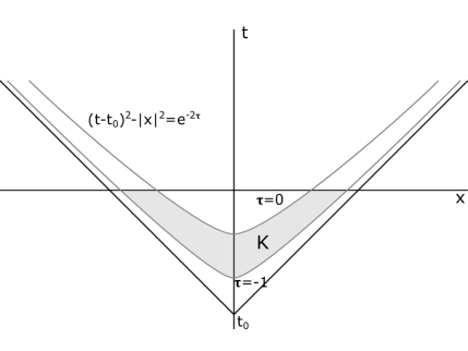
Figure 1: Illustration of region $K$

Small radius part

Now we need to consider the upper bound of $\displaystyle\inf_{\tau\in[-1,0]}E_{0}^{(2)}(\tau)$, which can be dominated by an integral

$$\inf_{\tau\in[-1,0]}E_{0}^{(2)}(\tau)\leq 2\pi\int_{-1}^{0}\int_{0}^{s_{0}(\tau)}\left[|v_{s}(s,\tau)|^{2}+|v_{\tau}(s,\tau)|^{2}\right]s^{2}ds\,d\tau$$

$$= \frac{1}{2}\int_{-1}^{0}\int_{0}^{s_{0}(\tau)}e^{-4\tau}\left(\frac{s}{\sinh s}\right)^{2}\left[|v_{s}(s,\tau)|^{2}+|v_{\tau}(s,\tau)|^{2}\right]4\pi e^{4\tau}\sinh^{2}s\,ds\,d\tau.$$

Let us recall our definition of $v$ and differentiate:

$$v_{\tau} =\frac{\sinh s}{s}e^{\tau}u+\frac{\sinh s\cosh s}{s}e^{2\tau}u_{t}+\frac{\sinh^{2}s}{s}e^{2\tau}u_{r};$$

$$v_{s} =\frac{s\cosh s-\sinh s}{s^{2}}e^{\tau}u+\frac{\sinh^{2}s}{s}e^{2\tau}u_{t}+\frac{\sinh s\cosh s}{s}e^{2\tau}u_{r}.$$

As a result we have

$$\left|\frac{s}{\sinh s}v_{\tau}\right| \leq\left\{|u|+(t-t_{0})|u_{t}|+r|u_{r}|\right\}_{(r,t)=(e^{\tau}\sinh s,t_{0}+e^{\tau}\cosh s)};$$

$$\left|\frac{s}{\sinh s}v_{s}\right| \leq\left\{|u|+r|u_{t}|+(t-t_{0})|u_{r}|\right\}_{(r,t)=(e^{\tau}\sinh s,t_{0}+e^{\tau}\cosh s)}.$$

Using these upper bounds and the change of variables formula (14), we obtain

$$\inf_{\tau\in[-1,0]}E_{0}^{(2)}(\tau) \lesssim\iint_{K}(1+t_{0}^{2})\left(|u_{t}|^{2}+|\nabla u|^{2}+|u|^{2}\right)dx\,dt$$

$$\lesssim(1+t_{0}^{2})\int_{-t_{0}}^{0}\int_{B(0,|t_{0}|)}\left(|u_{t}|^{2}+|\nabla u|^{2}+|u|^{p+1}+1\right)dx\,dt$$

$$\lesssim(1+t_{0}^{2})t_{0}^{4}+(1+t_{0}^{2})t_{0}\tilde{E}\lesssim_{A,\varepsilon}1.$$

Here the region $K=\{(x,t):e^{-2}\leq(t-t_{0})^{2}-|x|^{2}\leq 1,t_{0}<t\leq 0\}\subseteq B(0,|t_{0}|)\times[-t_{0},0]$, as illustrated in figure 1. The letter $\tilde{E}$ represents the energy of solution $u$, whose upper bound has been given in Remark 1.4. Combining the small radius part with the large radius part, we have

$$\inf_{t\in[-1,0]}E_{0}(\tau)\leq\sup_{t\in[-1,0]}E_{0}^{(1)}(\tau)+\inf_{t\in[-1,0]}E_{0}^{(2)}(\tau)\lesssim_{A,\varepsilon}1$$

thus finish the proof of Lemma 6.1.

6.2 A global integral estimate

Now $v$ is a radial solution to (CP2) with a finite energy $E(0)\lesssim_{A,\varepsilon}1$. We claim

$$I^{\prime}\doteq\int_{0}^{\infty}\!\!\int_{{\mathbb{R}}^{3}}e^{-(p-3)\tau}\left(\frac{|y|}{\sinh|y|}\right)^{p-1}|v(y,\tau)|^{2(p-1)}dy\,d\tau\lesssim_{A,\varepsilon,p}1.$$ (17)

Proof.

First of all, Proposition 3.4 gives a Morawetz-type estimate

$$\int_{0}^{\infty}\!\!\int_{{\mathbb{R}}^{3}}e^{-(p-3)\tau}\frac{|y|^{p-1}\cosh|y|}{\sinh^{p}|y|}|v(y,\tau)|^{p+1}dy\,d\tau\lesssim_{1}E(0)\lesssim_{A,\varepsilon}1.$$

Since $v(\cdot,\tau)$ is a radial $\dot{H}^{1}({\mathbb{R}}^{3})$ function, we also have

$$\left|v(y,\tau)\right|\lesssim\frac{\|v(\cdot,\tau)\|_{\dot{H}^{1}({\mathbb{R}}^{3})}}{|y|^{1/2}}\lesssim\frac{(E(\tau))^{1/2}}{|y|^{1/2}}\lesssim_{A,\varepsilon}\left(\frac{\cosh|y|}{\sinh|y|}\right)^{1/2}.$$

A combination of these two inequalities gives

$$\int_{0}^{\infty}\!\!\int_{{\mathbb{R}}^{3}}e^{-(p-3)\tau}\left(\frac{|y|}{\sinh|y|}\right)^{p-1}|v(y,\tau)|^{p+3}dy\,d\tau\lesssim_{A,\varepsilon}1.$$ (18)

If $p=3$, this is exactly the same inequality as (17). On the other hand, if $p\in(3,5)$, then we are able to apply Proposition 3.3 and obtain another integral estimate

$$\int_{0}^{\infty}\int_{{\mathbb{R}}^{3}}e^{-(p-3)\tau}\left(\frac{|y|}{\sinh|y|}\right)^{p-1}|v(y,\tau)|^{p+1}dy\,d\tau\leq\frac{p+1}{p-3}E(0)\lesssim_{A,\varepsilon,p}1.$$ (19)

Finally we can apply an interpolation between the inequalities (18) and (19) to conclude the proof, because our assumption $p\in(3,5)$ implies that $p+1<2(p-1)<p+3$. ∎

6.3 Completion of the proof for the main theorem

We have already known that the solution is well-defined for all time $t\in{\mathbb{R}}$. According to Proposition 3.7, it suffices to show

$$I\doteq\int_{0}^{\infty}\int_{{\mathbb{R}}^{3}}|u(x,t)|^{2(p-1)}dx\,dt\lesssim_{A,\varepsilon,p}1.$$

We first break the integral into two parts

$$I =\int_{0}^{\infty}\int_{|x|>t+R}|u(x,t)|^{2(p-1)}dx\,dt+\int_{0}^{\infty}\int_{|x|<t+R}|u(x,t)|^{2(p-1)}dx\,dt$$

$$\leq\int_{0}^{\infty}\int_{|x|>t+R}|u(x,t)|^{2(p-1)}dx\,dt+\iint_{\Omega}|u(x,t)|^{2(p-1)}dx\,dt\doteq I_{1}+I_{2}.$$

Here the region $\Omega=\{(x,t):|x|^{2}<(t-t_{0})^{2}-1,t>t_{0}\}$ satisfies (Please see figure 2)

• $\Omega$ contains the region $\{(x,t):|x|<t+R,t\geq 0\}$;

• $\Omega$ corresponds to the positive-time part of the $y$-$\tau$ space-time. In other words we have $\Omega=\mathbf{\tilde{T}}(\{(y,\tau):\tau>0\})$.

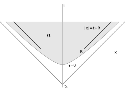
Figure 2: Illustration of the region $\Omega$

It is clear that $I_{1}\lesssim_{A,\varepsilon,p}1$ since the inequality $u(r,t)\lesssim_{A,\varepsilon}r^{-1}(r-t)^{-\delta}$ (when $r>t+R$ and $t\geq 0$) implies that

$$I_{1}\lesssim_{A,\varepsilon}\int_{0}^{\infty}\!\!\int_{t+R}^{\infty}[r^{-1}(r-t)^{-\delta}]^{2(p-1)}r^{2}\,drdt=\int_{R}^{\infty}\int_{s}^{\infty}r^{-2(p-2)}s^{-2(p-1)\delta}\,drds\lesssim_{A,\varepsilon}1.$$

In order to deal with $I_{2}$ we apply the change of variables formula (14).

$$I_{2}= \int_{0}^{\infty}\int_{{\mathbb{R}}^{3}}\left(e^{-\tau}\frac{|y|}{\sinh|y|}\right)^{2(p-1)}\left|\frac{\sinh|y|}{|y|}e^{\tau}u(\mathbf{\tilde{T}}(y,s))\right|^{2(p-1)}\cdot e^{4\tau}\left(\frac{\sinh|y|}{|y|}\right)^{2}dy\,d\tau$$

$$= \int_{0}^{\infty}\int_{{\mathbb{R}}^{3}}e^{-2(p-3)\tau}\left(\frac{|y|}{\sinh|y|}\right)^{2p-4}|v(y,\tau)|^{2(p-1)}dy\,d\tau.$$

The last expression of $I_{2}$ is different from the left hand of (17) (i.e. the integral $I^{\prime}$) only in the first two exponents. A simple comparison shows that $I_{2}\leq I^{\prime}\lesssim_{A,\varepsilon,p}1$. This finishes the proof of our main theorem.

References

- [1] J-P. Anker, V. Pierfelice, and M. Vallarino. “The wave equation on hyperbolic spaces” Journal of Differential Equations 252(2012): 5613-5661.
- [2] B. Dodson and A. Lawrie. “Scattering for the radial 3d cubic wave equation.” Analysis and PDE, 8(2015): 467-497.
- [3] T. Duyckaerts, C.E. Kenig, and F. Merle. “Scattering for radial, bounded solutions of focusing supercritical wave equations.” (2012): preprint arXiv: 1208.2158.
- [4] J. Ginibre, A. Soffer and G. Velo. “The global Cauchy problem for the critical nonlinear wave equation” Journal of Functional Analysis 110(1992): 96-130.
- [5] J. Ginibre, and G. Velo. “Conformal invariance and time decay for nonlinear wave equations.” Annales de l’institut Henri Poincaré (A) Physique théorique 47(1987), 221-276.
- [6] J. Ginibre, and G. Velo. “Generalized Strichartz inequality for the wave equation.” Journal of Functional Analysis 133(1995): 50-68.
- [7] M. Grillakis. “Regularity and asymptotic behaviour of the wave equation with critical nonlinearity.” Annals of Mathematics 132(1990): 485-509.
- [8] K. Hidano. “Conformal conservation law, time decay and scattering for nonlinear wave equation” Journal D’analysis Mathématique 91(2003): 269-295.
- [9] L. Kapitanski. “Weak and yet weaker solutions of semilinear wave equations” Communications in Partial Differential Equations 19(1994): 1629-1676.
- [10] C. E. Kenig, and F. Merle. “Global Well-posedness, scattering and blow-up for the energy critical focusing non-linear wave equation.” Acta Mathematica 201(2008): 147-212.
- [11] C. E. Kenig, and F. Merle. “Global well-posedness, scattering and blow-up for the energy critical, focusing, non-linear Schrödinger equation in the radial case.” Inventiones Mathematicae 166(2006): 645-675.
- [12] C. E. Kenig, and F. Merle. “Nondispersive radial solutions to energy supercritical non-linear wave equations, with applications.” American Journal of Mathematics 133, No 4(2011): 1029-1065.
- [13] R. Killip, and M. Visan. “The defocusing energy-supercritical nonlinear wave equation in three space dimensions” Transactions of the American Mathematical Society, 363(2011): 3893-3934.
- [14] H. Lindblad, and C. Sogge. “On existence and scattering with minimal regularity for semi-linear wave equations” Journal of Functional Analysis 130(1995): 357-426.
- [15] R. Shen. “On the energy subcritical, nonlinear wave equation in with radial data” Analysis and PDE 6(2013): 1929-1987.
- [16] R. Shen and G. Staffilani. “A Semi-linear Shifted Wave Equation on the Hyperbolic Spaces with Application on a Quintic Wave Equation on ”, to appear in Transactions of the American Mathematical Society, preprint arXiv: 1402.3879.
- [17] R. Shen. “On the energy-critical semi-linear shifted wave equation on the hyperbolic spaces”, preprint arXiv: 1408.0331.
- [18] D. Tataru. “Strichartz estimates in the hyperbolic space and global existence for the similinear wave equation” Transactions of the American Mathematical Society 353(2000): 795-807.