Quantum signature for laser-driven correlated excitation of Rydberg atoms

Abstract

The excitation dynamics of a laser-driven Rydberg atom system exhibits cooperative effect due to the interatomic Rydberg-Rydberg interaction, but the large many-body system with inhomogeneous Rydberg coupling is hard to be exactly solved or numerically studied by density matrix equations. In this paper, we find that the laser-driven Rydberg atom system with most of the atoms being in the ground state can be described by a simplified interaction model resembling the optical Kerr effect if the distance-dependent Rydberg-Rydberg interaction is replaced by an infinite-range coupling. We can then quantitatively study the effect of the quantum fluctuations on the Rydberg excitation with the interatomic correlation involved and analytically calculate the statistical characteristics of the excitation dynamics in the steady state, revealing the quantum signature of the driven-dissipative Rydberg atom system. The results obtained here will be of great interest for other spin-1/2 systems with spin-spin coupling.

I Introduction

A laser-driven Rydberg gas in which the Rydberg excited atoms experience the long-ranged dipole-dipole or van der Waals interaction potential can exhibit atomic many-body correlations that are of great interest for future applications in quantum information processing Saffman et al. (2010) and quantum nonlinear optics Chang et al. (2014). While much attention has been recently devoted to the enhancement of optical nonlinearity by mapping the Rydberg-Rydberg correlation onto optical field Pritchard et al. (2010); Sevinçli et al. (2011); Petrosyan et al. (2011); Peyronel et al. (2012); Parigi et al. (2012); Yan et al. (2012); Gorshkov et al. (2013); Maxwell et al. (2013); He et al. (2014); Li et al. (2014); Maghrebi et al. (2015) and to the nonequilibrium quantum phenomena Weimer et al. (2008); Weimer and Büchler (2010); Lee et al. (2011); Qian et al. (2012); Lesanovsky and Garrahan (2013); Marcuzzi et al. (2014); Hoening et al. (2014) and the preparation of Rydberg crystals Glaetzle et al. (2012); Höning et al. (2013); Vermersch et al. (2015) by modulating the driven-dissipative dynamics, the quantitative understanding of the excitation process for the Rydberg atom system itself is of particular interest on the other hand and is not yet clear.

There has been a lot of theoretical work focusing on the excitation dynamics in both the coherent Ates et al. (2007a, b); Mayle et al. (2011); Ates and Lesanovsky (2012); Petrosyan et al. (2013); Gärttner et al. (2013); Bettelli et al. (2013); Sanders et al. (2015) and dissipative regimes Ates et al. (2012); Lee and Cross (2012); Lee et al. (2012); Hu et al. (2013); Schönleber et al. (2014); Gärttner et al. (2014); Olmos et al. (2014); Weimer (2015); Schempp et al. (2015). Generally, the system was analyzed via a mean-field treatment disregarding the interatomic correlation Ates et al. (2012); Marcuzzi et al. (2014); Olmos et al. (2014); Vermersch et al. (2015); Lesanovsky and Garrahan (2013), a variational approach allowing for an approximation of the true steady state Weimer (2015) or a perturbation theory up to fourth order Lee and Cross (2012); Gärttner et al. (2014); Schempp et al. (2015). Alternatively, the incoherent dynamics can be numerically simulated on account of strong dissipation via the rate equation Ates et al. (2007b); Schönleber et al. (2014), and weak decay via the density-matrix master equation Petrosyan et al. (2013) (or equivalently the wave-function Monte Carlo approach Lee and Cross (2012); Lee et al. (2012); Hu et al. (2013); Olmos et al. (2014); Schönleber et al. (2014)) and the density-matrix renormalization-group Höning et al. (2013) that are normally useful for the lattice geometrics consisting of several tens of atoms.

The excitation dynamics under resonant and off-resonant driving exhibits different counting statistics of the Rydberg atom number. While the resonant driving leads to reduced number fluctuations of the Rydberg excitations Viteau et al. (2012); Hofmann et al. (2013); Bettelli et al. (2013), the off-resonant coupling offers richer physics such as the experimentally observed optical bistability Carr et al. (2013), Rydberg aggregates Schempp et al. (2014); Urvoy et al. (2015), bimodal counting distribution Malossi et al. (2014), and kinetic constraints Valado et al. (2015). In addition, of special interest for the experimental analysis is the formation mechanism of the collective many-body states since the statistical characteristics Schempp et al. (2014); Malossi et al. (2014) and direct imaging Günter et al. (2012); Schwarzkopf et al. (2011) are challenging for distinguishing sequential and simultaneous excitation process of the Rydberg atoms. These have also been theoretically studied via the analytical model with generalized Dicke states Viteau et al. (2012) or Monte Carlo simulation Schempp et al. (2014).

In this paper, we study the excitation dynamics of a laser driven-dissipative Rydberg atom system in the Holstein-Primakoff regime, i.e. the majority of atoms remain in the ground state Schempp et al. (2014); Malossi et al. (2014). To give an intuitive understanding, we make use of a simplified picture for the many-body system as in ref. Lee et al. (2012), where the characteristic $C_{\mu}/R^{\mu}$ ($\mu=3,6$) dependent interaction for atom pairs with the separation $R$ is replaced by an infinite-range coupling (or average pair interaction). It allows us to regard the system as a nonlinear optical polarizability model Drummond and Walls (1980) and quantitatively study the effect of quantum correlations on the excitation dynamics in the steady state. We find from the linearized calculation that the quantum fluctuations to the first order will enhance the Rydberg population Lee et al. (2012); Gärttner et al. (2014) and modulate the fluctuation of the collective excitation number. Moreover, the nonclassical effects like pair excitation of Rydberg atoms can be clearly revealed by the full quantum results after comparison with the classical steady-state solution. The limitations for this simplified model are also discussed. Our finding not only connects to the recent experimental observations for the many-body system with Rydberg-Rydberg coupling Labuhn et al. (2016), but also relates to the trapped spin-$1/2$ ions system where the spin-spin couplings are mediated by the motional degrees of freedom Britton et al. (2012).

The paper is organized as follows. In Sec. II, we introduce our model for the interacting Rydberg atoms in the Holstein-Primakoff regime. In Sec. III, we numerically solve the classical Langevin equation of motion for the Rydberg atom system to study the bistability of Rydberg population. In section IV, we discuss the effect of quantum fluctuations on the Rydberg excitation dynamics in the linearized regime. In section V, we give the exact steady-state solution of the Fokker-Planck equation for describing the full quantum dynamics. Section VI finally contains a summary of our results and an open discussion of the limitations for the model.

II Theoretical Model

Consider a system of $N$ atoms ($N\gg 1$) that are excited from the ground state $|g_{j}\rangle$ to a Rydberg state $|e_{j}\rangle$ by a continuous and spatially uniform laser beam with the detuning $\Delta$ from atomic resonance and the Rabi frequency $\Omega$ (assumed to be real). By including the all-to-all interatomic coupling (or average pair interaction) $\chi$, the Hamiltonian in the interaction picture and rotating-wave approximation reads ($\hbar=1$) Lee et al. (2012)

$$H = \sum_{j=1}^{N}\left[-\Delta|e_{j}\rangle\langle e_{j}|+\frac{\Omega}{2}(|e_{j}\rangle\langle g_{j}|+|g_{j}\rangle\langle e_{j}|)\right]$$ (1)

$$+\chi\sum_{j<k}|e_{j}\rangle\langle e_{j}|\otimes|e_{k}\rangle\langle e_{k}|.$$

We now introduce the collective spin operators $S^{+}=\sum_{j=1}^{N}|e_{j}\rangle\langle g_{j}|$ and $S^{-}=\sum_{j=1}^{N}|g_{j}\rangle\langle e_{j}|$, which according to the Holstein-Primakoff transformation can be expressed in terms of the bosonic operators $b$ and $b^{\dagger}$ (with $[b,b^{\dagger}]=1$) as $S^{+}=b^{\dagger}\sqrt{N-b^{\dagger}b}$ and $S^{-}=\sqrt{N-b^{\dagger}b}b$ if the lowest energy level of these new operators is set to be the atomic state in which all of the atoms are in the ground state Sun et al. (2003); Hammerer et al. (2010). It follows that $\sum_{j=1}^{N}|e_{j}\rangle\langle e_{j}|=\frac{1}{2}[S^{+},S^{-}]+\frac{N}{2}=b^{\dagger}b$ and $\sum_{j<k}|e_{j}\rangle\langle e_{j}|\otimes|e_{k}\rangle\langle e_{k}|=\frac{1}{2}b^{\dagger}b^{\dagger}bb$. We then focus on the parameter regime where the mean number of Rydberg excitations is much less than the total number of atoms (i.e. $\bar{n}_{e}\equiv\langle b^{\dagger}b\rangle\ll N$) resulting in $S^{+}\simeq\sqrt{N}b^{\dagger}$, $S^{-}\simeq\sqrt{N}b$ Schempp et al. (2014); Malossi et al. (2014). Thus, the Hamiltonian of the system can be rewritten by

$$H_{b} = -\Delta b^{\dagger}b+\frac{\chi}{2}b^{\dagger}b^{\dagger}bb+\lambda(b+b^{\dagger})$$ (2)

with $\lambda=\sqrt{N}\Omega/2$. Note that the system involving the Rydberg-Rydberg coupling behaves in resemblance to the optical Kerr nonlinearity and its coherent dynamics will remain in the symmetric Dicke state space. However, the spontaneous decay from the Rydberg excited state (with the relaxation rate $\gamma$) may lead to incoherent mixture with the asymmetric dark states. For clarity, our work will focus on the state space mainly spanned by null and single Rydberg excitation accompanied by a tiny fraction of double excitations. The Rydberg population is confirmed by direct simulations of the master equation $\dot{\rho}=-i[H_{b},\rho]+\frac{\gamma}{2}(2b\rho b^{\dagger}-\rho b^{\dagger}b-b^{\dagger}b\rho)$ for a zero-temperature thermal reservoir, and the counting statistics of Rydberg excitation is quantified by the Mandel $Q$ parameter defined as $Q=\langle(\Delta\hat{n}_{e})^{2}\rangle/\langle\hat{n}_{e}\rangle-1$ with $\hat{n}_{e}\equiv b^{\dagger}b$, as shown in Fig. 1. The exact simulation of the dissipative dynamics for few atoms with the Hamiltonian Eq. (1) can be found in Appendix A, which shows good agreement with the bosonization model. But it should also be mentioned that for a realistic Rydberg system, such as an atomic ensemble or a spin lattice, the finite interaction range and the continuum of interatomic coupling strengths due to broad distribution of atom position may induce loss of interatomic correlations, which may negate the effectiveness of the model.

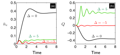
Figure 1: (Color online) (a) Mean Rydberg population $\bar{n}_{e}$ and (b) Mandel $Q$ parameter as a function of time for laser detunings $\Delta=-5$, $0$ and $5$ respectively. We fix units of $\gamma=1,$ taking $\lambda=0.6$, $\chi=10$. In all cases the population of the double-excitation state is less than $0.01$. For $\Delta=5$, the Rydberg excitation exhibits super-Poissonian counting statistics with $Q>0$, while for $\Delta=-5$ and $\Delta=0$, the sub-Poissonian processes characterized by $Q<0$ are found.

III Classical dynamics

The quantum Langevin equation of motion for the bosonic system is

$$\dot{b} = -i\lambda-i\Gamma b-i\chi b^{\dagger}b^{2}+\xi(t)$$ (3)

where $\Gamma=-(\Delta+i\gamma/2)$ might include the decoherence due to the laser linewidths and doppler broadening, and $\xi(t)$ is the zero-value-mean noise operator. Beyond the mean-field theory, here the correlation between atoms is retained in the evolutional dynamics. In the classical limit, the equation of motion for $\bar{\alpha}=\langle b\rangle$ ($\bar{\alpha}^{*}=\langle b^{\dagger}\rangle$) are given by

$$\dot{\bar{\alpha}}=-i\lambda-i\bar{\alpha}(\Gamma+\chi|\bar{\alpha}|^{2}),$$

$$\dot{\bar{\alpha}}^{*}=i\lambda+i\bar{\alpha}^{*}(\Gamma^{*}+\chi|\bar{\alpha}|^{2}).$$ (4)

Then, the mean number of Rydberg excitations $\bar{n}_{es}=|\bar{\alpha}_{s}|^{2}$ in the steady state fulfills the algebraic equation

$$\chi^{2}\bar{n}_{es}^{3}-2\chi\Delta\bar{n}_{es}^{2}+\bar{n}_{es}|\Gamma|^{2}-\lambda^{2}=0$$ (5)

that allows at most three real positive roots. A stable $\bar{n}_{es}$ must conform to the Hurwitz criterion (given by $\partial(\lambda^{2})/\partial\bar{n}_{es}=3\chi^{2}\bar{n}_{es}^{2}-4\bar{n}_{es}\chi\Delta+|\Gamma|^{2}>0$ here), which ensures that the system returns to the stable branch soon after the small perturbation. Therefore, if the conditions $|\Delta|>\sqrt{3}\gamma/2$ and $\Delta\chi>0$ are satisfied, the bistable region will be given by $\bar{n}_{es}>\bar{n}_{es}^{(+)}$ or $\bar{n}_{es}<\bar{n}_{es}^{(-)}$ with the real positive $\bar{n}_{es}^{(\pm)}=(2\Delta\pm\sqrt{\Delta^{2}-\frac{3}{4}\gamma^{2}})/3\chi$. For our interest, the dependence of $\bar{n}_{es}$ on the laser detuning $\Delta$ for a repulsive interatomic interaction ($\chi>0$) is shown in Fig. 2(b), which exhibits optical bistability with hysteresis Carr et al. (2013). The coexistence of a low and a high Rydberg population in the off-resonance regime ($\Delta>0$) leads to the bimodal counting distributions of the Rydberg excitation Malossi et al. (2014). While for $\Delta=0$, the bimodality can not arise due to the impossible bistability.

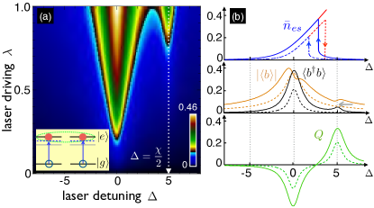
Figure 2: (Color online) (a) Mean number of Rydberg excitations $\langle b^{\dagger}b\rangle$ in the steady state with full quantum theory as a function of $\lambda$ and $\Delta$. The inset shows the pair excitation of two atoms for $\Delta=\chi/2$. (b) Classical stationary mean $\bar{n}_{es}$, quantum mechanical steady-state solution of $\langle b^{\dagger}b\rangle$ and $|\langle b\rangle|$, and Mandel $Q$ parameter versus laser detuning $\Delta$ with $\lambda=0.3$ (dash) and $\lambda=0.6$ (solid). Further parameters as in Fig. 1. $\chi$, $\lambda$ and $\Delta$ are in units of $\gamma$.

IV Linearized dynamics

The dissipative quantum dynamics for the system can be described by the master equation or the corresponding Fokker-Planck equation (FPE) Drummond and Walls (1980)

$$\dot{P}(\alpha,\beta,t) = i[\frac{\partial}{\partial\alpha}(\Gamma\alpha+\chi\alpha^{2}\beta+\lambda)-\frac{\chi}{2}\frac{\partial^{2}}{\partial\alpha^{2}}\alpha^{2}$$

$$-\frac{\partial}{\partial\beta}(\Gamma^{*}\beta+\chi\beta^{2}\alpha+\lambda)+\frac{\chi}{2}\frac{\partial^{2}}{\partial\beta^{2}}\beta^{2}]P(\alpha,\beta,t)$$

by introducing the non-diagonal generalized $P$ representation defined by

$$\rho(t)=\int_{D}d\sigma(\alpha,\beta)P(\alpha,\beta,t)\frac{|\alpha\rangle\langle\beta^{*}|}{\langle\beta^{*}|\alpha\rangle},$$ (7)

where $D$ is the integration domain, and $d\sigma$ is the integration measure that can be a volume integral $d^{2}\alpha d^{2}\beta$ over a complex phase space or a line integral $d\alpha d\beta$ over a manifold embedded in a complex phase space Drummond and Walls (1980). Note that $\alpha$, $\beta$ are arguments of the generalized $P$ function (in correspondence to the $c$ numbers of $b$, $b^{\dagger}$) and are complex conjugate in the mean $\bar{\alpha}=\bar{\beta}^{*}$.

Transforming the FPE into the Ito form yields a pair of stochastic differential equations (SDEs):

$$\frac{\partial}{\partial t}\left[\begin{array}[]{c}\alpha\\ \beta\end{array}\right] = \left[\begin{array}[]{c}-i(\Gamma\alpha+\chi\alpha^{2}\beta+\lambda)\\ i(\Gamma^{*}\beta+\chi\beta^{2}\alpha+\lambda)\end{array}\right]$$ (17)

$$+\left[\begin{array}[]{cc}-i\chi\alpha^{2}&0\\ 0&i\chi\beta^{2}\end{array}\right]^{\frac{1}{2}}\left[\begin{array}[]{c}\xi_{1}(t)\\ \xi_{2}(t)\end{array}\right]$$

with $\xi_{1,2}(t)$ the delta-correlated Gaussian white noise, satisfying $\langle\xi_{1,2}(t)\rangle=0$ and $\langle\xi_{1,2}(t)\xi_{1,2}(t^{\prime})\rangle\sim\delta(t-t^{\prime})$. We then linearize the SDEs around the classically steady-state solution $\bar{\alpha}_{s}(\bar{\beta}_{s}=\bar{\alpha}_{s}^{*})$, and find that the quantum fluctuation $\delta\mathbf{\hat{X}}=[\delta\hat{\alpha},\delta\hat{\beta}]^{T}$ close to the classical stable branches obeys the equation

$$\delta\dot{\mathbf{\hat{X}}}=-\mathbf{\boldsymbol{\mu}}(\bar{\alpha}_{s})\cdot\mathbf{\delta\mathbf{\hat{X}}}+\mathbf{D}^{1/2}(\bar{\alpha}_{s})\cdot\boldsymbol{\xi}(t),$$ (18)

where

$$\boldsymbol{\mathbf{\mu}}(\bar{\alpha}_{s})=-i\left[\begin{array}[]{cc}\Gamma+2\chi|\bar{\alpha}_{s}|^{2}&-\chi\bar{\alpha}_{s}^{*2}\\ \chi\bar{\alpha}_{s}^{2}&-\Gamma-2\chi|\bar{\alpha}_{s}|^{2}\end{array}\right]$$ (19)

and

$$\mathbf{D}(\bar{\alpha}_{s})=\left[\begin{array}[]{cc}-i\chi\bar{\alpha}_{s}^{2}&0\\ 0&i\chi\bar{\alpha}_{s}^{*2}\end{array}\right]$$ (20)

are the linearized drift and the diffusion array, respectively. The correlation matrix with regard to $\delta\mathbf{\hat{X}}$ can now be calculated through

$$\mathbf{C} = \left[\begin{array}[]{cc}\langle b^{2}\rangle-\langle b\rangle^{2}&\langle b^{\dagger}b\rangle-|\langle b\rangle|^{2}\\ \langle b^{\dagger}b\rangle-|\langle b\rangle|^{2}&\langle b^{\dagger 2}\rangle-\langle b^{\dagger}\rangle^{2}\end{array}\right]$$ (23)

$$= \frac{\mathbf{D}\cdot\textrm{Det}(\mathbf{\boldsymbol{\mu}})+[\boldsymbol{\mu-}\mathbf{I}\cdot\textrm{Tr}(\boldsymbol{\mu})]\mathbf{D}[\boldsymbol{\mu-}\mathbf{I}\cdot\textrm{Tr}(\boldsymbol{\mu})]^{T}}{2\textrm{Tr}(\boldsymbol{\mu})\textrm{Det}(\boldsymbol{\mu})}.$$ (24)

The above result allows us to obtain the mean Rydberg population and the Mandel $Q$ parameter in the linearized regime: (see Appendix B)

$$\bar{n}_{e} \approx |\bar{\alpha}_{s}|^{2}+\langle\delta\hat{\alpha}^{\dagger}\delta\hat{\alpha}\rangle=\bar{n}_{es}+\frac{\chi^{2}}{2\Lambda}\bar{n}_{es}^{2},$$ (25)

$$Q \approx 2\bar{n}_{es}\textrm{Re}[\langle\delta\hat{\alpha}^{2}\rangle/\bar{\alpha}_{s}^{2}]+2\langle\delta\hat{\alpha}^{\dagger}\delta\hat{\alpha}\rangle$$ (26)

$$= \frac{\bar{n}_{es}\chi}{\Lambda}(\Delta-\chi\bar{n}_{es}),$$

with $\Lambda=|\Gamma|^{2}-4\chi\Delta\bar{n}_{es}+3\chi^{2}\bar{n}_{es}^{2}.$ The steady-state solution $\bar{n}_{es}$ can be obtained by solving the set of classically nonlinear equations (4), and there may exist two stable solution for a well-selected laser detuning as shown in Fig.2(b). We now assume this solution has been found and focus on the effect of the quantum fluctuations. One of the intriguing effects can be found in the asymptotic expansion of $\bar{n}_{e}$ to the first-order [see Eq. (25)], where the Rydberg population is enhanced by the Rydberg-Rydberg coupling via the intensity of quantum fluctuation $\langle\delta\hat{\alpha}^{\dagger}\delta\hat{\alpha}\rangle$ Lee et al. (2012); Gärttner et al. (2014). Second, due to the Rydberg-Rydberg interactions, the laser field drives the atomic transition from the ground state to the Rydberg state in a cooperative manner, with the fluctuations of the collective excitation number being characterized by the Mandel $Q$ factor. The results show that the collective excitation number exhibits super-Poissonian distribution for the laser detuning $\Delta$ greater than the collective energy shift $\bar{n}_{es}\chi$ among the correlated interacting particles ($\Delta/\bar{n}_{es}\chi>1$) and sub-Poissonian distribution for the other ($\Delta/\bar{n}_{es}\chi<1$), leading to collective quantum jumps while the system stays in the two classically stable branches Lee et al. (2012). The linear theory breaks down for $\Lambda\rightarrow 0$ (corresponding to the violation of the Hurwitz criterion), in which case $\bar{n}_{es}$ approaches the onset of instability.

V Full quantum dynamics

Having seen the effect of the quantum fluctuations based on the linearization, we next address the question with full quantum theory. In the quantum noise limit, there exists an exact steady-state solution $P_{ss}(\alpha,\beta)=\alpha^{c-2}\beta^{d-2}exp[-z(1/\alpha+1/\beta)+2\alpha\beta$ for the FPE (LABEL:eq:FPE) with $z=2\lambda/\chi,$ $c=2\Gamma/\chi$, and $d=c^{*}$ (see Appendix C). While we obtain the generalized $P$ function, the Rydberg population and the Rydberg counting statistics can be calculated via

$$\langle b^{\dagger n}b^{m}\rangle=\frac{\int_{D}d\sigma(\alpha,\beta)P_{ss}(\alpha,\beta)\beta^{n}\alpha^{m}}{\int_{D}d\sigma(\alpha,\beta)P_{ss}(\alpha,\beta)}.$$ (27)

The appropriate integration domain $D$ here will be a complex manifold embedded in the space $\mathbb{C}^{2}$ and each path of integration is chosen to be a Hankel path $\mathcal{O}$. These ensure that the distribution function $P(\alpha,\beta)$ vanishes correctly at the boundary. Skipping over the fussy calculations we finally come at (see Appendix C)

$$\langle b\rangle=\frac{z}{c}\frac{{}_{0}F_{2}(c+1,d,2z^{2})}{{}_{0}F_{2}(c,d,2z^{2})},$$ (28)

$$\langle b^{\dagger}b\rangle=\frac{z^{2}}{cd}\frac{{}_{0}F_{2}(c+1,d+1,2z^{2})}{{}_{0}F_{2}(c,d,2z^{2})},$$ (29)

$$Q = \frac{z^{2}}{(c+1)(d+1)}\frac{{}_{0}F_{2}(c+2,d+2,2z^{2})}{{}_{0}F_{2}(c+1,d+1,2z^{2})}$$ (30)

$$-\frac{z^{2}}{cd}\frac{{}_{0}F_{2}(c+1,d+1,2z^{2})}{{}_{0}F_{2}(c,d,2z^{2})},$$

where ${}_{0}F_{2}(c,d,z)$ is a hypergeometric series defined as

$${}_{0}F_{2}(c,d,z)=\sum_{n=0}^{\infty}\frac{z^{n}}{n!}\frac{\Gamma(c)\Gamma(d)}{\Gamma(c+n)\Gamma(d+n)}$$ (31)

with $\Gamma(x)=[\frac{z^{1-x}}{2\pi i}\int_{\mathcal{O}}\sigma{}^{-x}e^{\sigma z}d\sigma]^{-1}$ the gamma-function.

The phase diagram for the mean number of Rydberg excitations in ($\lambda,\Delta$) space shows that the Rydberg excitation dramatically increases at the laser detunings $\Delta=0$ and $\Delta=\chi/2$ [see Fig. 2(a)], which corresponds to individually resonant excitation of the each atom and pair excitation of the interacting atoms, respectively. Numerical simulation proves that the system is confined in the subspace spanned by the null- and double-excitation states for $\Delta=\chi/2$ without considering the relaxation, confirming that for this detuning the atomic excitation is caused by the two-photon process; this is fundamentally different from the case of resonant driving, where the system has no probability of being pumped to the state with more than one excitation due to the Rydberg blockade. Taking into account the atomic spontaneous emission, the issue whether the many-body states of the Rydberg atoms are created by the coherent two-photon process or sequential excitations of individual atoms is then determined by the sequential to two-photon ratio, which is proportional to $\gamma^{2}/N\Omega^{2}$ Schempp et al. (2014). Thus, the system favors double excitation since the multiatom coherence becomes significant and the dephasing induced by random distribution of atom position and specific spatial laser profile is neglected Schönleber et al. (2014). This can be further confirmed by measuring the Mandel $Q$ parameter that is in close relation to the spatial correlation function $g^{(2)}(R)$ Wüster et al. (2010). The excitation processes exhibit the sub-Poissonian character ($Q<0$) on resonance and super-Poissonian character ($Q>0$) for the other. Besides, due to the fact that the interatomic correlations between any pairs of atoms are included, the cooperative transitions from the doubly excitation state to the higher excitation states are largely detuned from resonance and are suppressed for the collective energy shifts being much larger than the laser driving strength.

For $0<\Delta<\chi/2$, both the individual excitation and the pair excitation are possible. While the classical dynamics predicts an optical bistability, the quantum mechanical calculation including the interatomic correlation does not exhibit bistability. It should also be noted that the pair excitation of two atoms is a nonclassical effect that is unable to be revealed by the classical theory [see arrow in Fig. 2(b)] (see Appendix D). An extra quantum signature for the system is given by the dips in the laser-detuning dependence of $|\langle b\rangle|$, which arise at the transition points of Mandel $Q$ factor that shows a reduced or enhanced quantum fluctuations of Rydberg excitations Lee et al. (2011); Ates et al. (2012); Lee et al. (2012).

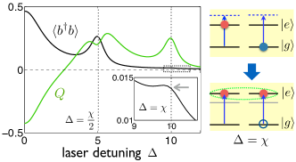
Figure 3: (Color online) Left panel: Quantum mechanical steady-state solution of mean Rydberg population $\langle b^{\dagger}b\rangle$ and Mandel $Q$ parameter versus laser detuning $\Delta$ with increasing driving strength $\lambda=1$ and $\chi=10$. $\chi$, $\lambda$ and $\Delta$ are in units of $\gamma$. Right panel: An already excited Rydberg atom forwards the excitation of the surrounding atoms interacting with it for $\Delta=\chi$. See the text for detail.

Increasing the laser intensity will enhance the mean number of Rydberg excitations for $\Delta=\chi/2$, but meanwhile weaken the super-Poissonian excitation process due to the decreasing ratio $\Delta/\bar{n}_{es}\chi$, as shown in Fig. 3. This fact can be directly understood from the linearized calculation Eq. (26)]. For the far off-resonance regime $\Delta\gg\Omega$, there is a small chance (roughly $N\Omega^{2}/4\Delta^{2}$) for an atom being excited to the Rydberg state if all the atoms are initially in the ground state. However, while an atom has been luckily excited by the laser beam with the detuning $\Delta=\chi$, then similar to the Rydberg aggregates, the surrounding atoms tend to be excited cooperatively due to the Rydberg-Rydberg coupling, as sketched in the right panel of Fig. 3. Besides, the sequential to simultaneous three-photon excitation ratio is on the order of $\gamma^{2}\Delta^{2}/N^{2}\Omega^{4}$ and is extremely weak here.

VI Discussion and Conclusion

As mentioned in Sec. II, the simplified picture here requires the interatomic correlations to be well preserved amongst the whole Rydberg ensemble, and the only scenario where the present model describes actual Rydberg atom interactions is when all interactions are so strong ($\chi\gg\Delta$ or $\lambda$) that the ensemble is fully blockaded, i.e. not even double excitations can ever occur. While the scale of a Rydberg atom system is much larger than the blockade radius (i.e. the critical correlation distance), the quantum correlations may vanish for Rydberg atoms seated far away from each other; then the situation becomes different for the Rydberg excitation number being related to the number of blockade spheres that fit into the excitation volume. The excitation dynamics for ultracold Rydberg gas with high atomic density has been experimentally studied in the strong dephasing regime (due to the spatial dependence of atom positions or laser geometry) and in the limit of short excitation times Schempp et al. (2014); Malossi et al. (2014).

It is more interesting to study the excitation dynamics in the scenario that $\chi$ is of a comparable order to $\Delta$ or $\lambda$ as employed here. The quantum correlations among all the atoms become essential, giving rise to the pronounced quantum signature discussed previously. But for actual experiments such as individual Rydberg atoms trapped in tunable two-dimensional arrays of optical microtraps Labuhn et al. (2016), the distance-dependent interatomic coupling strength is determined by the specific lattice sites that the atoms locate on, and therefore the factor of 8 (or higher) difference in interactions comparing two adjacent atoms already introduces correlations and breaks the present approach. This is regardless of the dimensionality or geometry of a lattice. However, the strong two-photon transitions will be still visible while many pairs of the atoms feature distance that fits in with the two-photon resonance condition, namely, the two-photon resonance can be enhanced by choosing the appropriate detuning for a given lattice constant Schönleber et al. (2014). The limitations arise from the fact that the atoms near the edge of lattice evolve as an inhomogeneous distribution of atom position, which breaks the spatial symmetry and may induce an additional dephasing reducing the visibility of two-photon transitions Labuhn et al. (2016).

In conclusion, we have analyzed the steady-state excitation dynamics of a weakly-driven Rydberg-atom system by treating the inhomogeneous Rydberg-Rydberg interaction as an all-to-all coupling. While the present model can not represent the full picture of a realistic system, in contrast to the previous analytical or experimental studies that mainly focus on the mean-field dynamics and neglect the interatomic correlations, the analytical calculation here allows us to find the effect of the quantum fluctuations on the Rydberg excitation process and the quantum phenomena such as simultaneous bi-excitation of Rydberg atoms and interaction-assisted Rydberg excitation, which are referred to as the quantum signature of the system. The simplified model forms the basis for quantitatively understanding the Rydberg aggregates Schempp et al. (2014); Urvoy et al. (2015), bimodal counting distribution Malossi et al. (2014), and kinetic constraints Valado et al. (2015) in recent experimental observations with Rydberg atoms, and more generally the many-body effect for the interacting spin-$1/2$ systems Britton et al. (2012).

Appendix A The exact simulation of the dissipative dynamics with atomic spin operators

In this section, we show that the exact simulation of the Hamiltonian $H$ in the main text with spin operators for few atoms is found to be in good agreement with the theoretical model in terms of bosonic operators. We also show how to obtain the correlation matrix under linearization and the analytical steady-state solution for the Fokker-Planck equation as in ref. Drummond and Walls (1980) discussing the optical bistability for nonlinear polarisability model. The nonclassical nature of the quantum mechanical steady states is also shown by the Wigner functions.

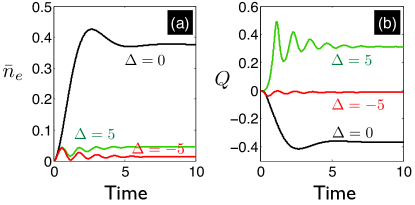
Figure 4: (Color online) (a) Mean Rydberg population $\bar{n}_{e}$ and (b) Mandel $Q$ parameter as a function of time for laser detunings $\Delta=-5$, $0$ and $5$ respectively. Further parameters as in Fig. 1 in the main text.

The exactly dissipative dynamics of the laser-driven system with the Hamiltonian $H$ in the main text can be described by the master equation

$$\dot{\rho}=\frac{1}{i\hbar}[H,\rho]+\frac{\gamma}{2}\sum_{j=1}^{N}\mathcal{L}_{j},$$ (32)

where

$$\mathcal{L}_{j}=2\sigma_{ge}^{(j)}\rho\sigma_{eg}^{(j)}-\sigma_{eg}^{(j)}\sigma_{ge}^{(j)}\rho-\rho\sigma_{eg}^{(j)}\sigma_{ge}^{(j)},$$ (33)

$\sigma_{ge}^{(j)}=|g_{j}\rangle\langle e_{j}|$ and $\sigma_{eg}^{(j)}=|e_{j}\rangle\langle g_{j}|$. With the excitation-number operator being $\hat{n}_{e}=\sum_{j=1}^{N}|e_{j}\rangle\langle e_{j}|$, the mean number of Rydberg excitations and the Mandel $Q$ parameter can be calculated via $\bar{n}_{e}=\textrm{Tr}(\rho\hat{n}_{e})$ and $Q=\textrm{Tr}(\rho(\Delta\hat{n}_{e})^{2})/\textrm{Tr}(\rho\hat{n}_{e})-1$, respectively.

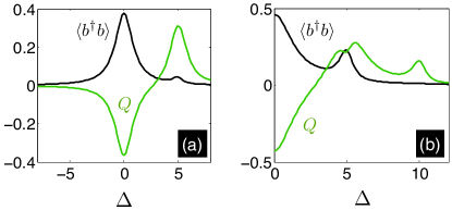
Figure 5: (Color online) Quantum mechanical steady-state solution of $\bar{n}_{e}$ and Mandel $Q$ parameter versus laser detuning $\Delta$ for (a) $\lambda=0.6$ and (b) $\lambda=1$. Further parameters as in Fig. 2(b) in the main text.

Simulating the Eq. (32) with $N=6$, we show the time-dependent mean Rydberg population $\bar{n}_{e}$ and Mandel $Q$ parameter in Fig. 4, and the steady-state solution of $\bar{n}_{e}$ and $Q$ versus laser detuning $\Delta$ in Fig. 5, which demonstrate the quantitatively good agreement with the results obtained via the simulation of the bosonization model.

Appendix B The quantum fluctuation under linearization

Splitting the operators $b$ ($b^{\dagger}$) into classical and quantum parts $\alpha=\bar{\alpha}+\delta\hat{\alpha}(t)$, $\beta=\bar{\beta}+\delta\hat{\beta}(t)$ ($\bar{\alpha}^{*}=\bar{\beta}$), we obtain the linearized correlation matrix given by

$$\mathbf{C} = \left[\begin{array}[]{cc}\langle b^{2}\rangle-\langle b\rangle^{2}&\langle b^{\dagger}b\rangle-|\langle b\rangle|^{2}\\ \langle b^{\dagger}b\rangle-|\langle b\rangle|^{2}&\langle b^{\dagger 2}\rangle-\langle b^{\dagger}\rangle^{2}\end{array}\right]$$ (36)

$$= \left[\begin{array}[]{cc}\langle\delta\hat{\alpha}^{2}\rangle&\langle\delta\hat{\alpha}^{\dagger}\delta\hat{\alpha}\rangle\\ \langle\delta\hat{\alpha}^{\dagger}\delta\hat{\alpha}\rangle&\langle\delta\hat{\alpha}^{\dagger 2}\rangle\end{array}\right]$$ (39)

where

$$\langle\delta\hat{\alpha}^{2}\rangle=-\frac{\chi\bar{\alpha}^{2}(\Gamma^{*}+2\chi\bar{n}_{es})}{2\Lambda},$$ (40)

$$\langle\delta\hat{\alpha}^{\dagger}\delta\hat{\alpha}\rangle=\frac{\chi^{2}\bar{n}_{es}^{2}}{2\Lambda}$$ (41)

and

$$\langle\delta\hat{\alpha}^{\dagger 2}\rangle=-\frac{\chi\bar{\alpha}^{*2}(\Gamma+2\chi\bar{n}_{es})}{2\Lambda}$$ (42)

with $\Lambda=\frac{\gamma^{2}}{4}+\Delta^{2}-4\chi\Delta\bar{n}_{es}+3\chi^{2}\bar{n}_{es}^{2}$ are obtained from $\mathbf{C}=\frac{\mathbf{D}\cdot\textrm{Det}(\mathbf{\boldsymbol{\mu}})+[\boldsymbol{\mu-}\mathbf{I}\cdot\textrm{Tr}(\boldsymbol{\mu})]\mathbf{D}[\boldsymbol{\mu-}\mathbf{I}\cdot\textrm{Tr}(\boldsymbol{\mu})]^{T}}{2\textrm{Tr}(\boldsymbol{\mu})\textrm{Det}(\boldsymbol{\mu})}$ by using the drift and diffusion arrays. Thus, the mean number of Rydberg excitations and the Mandel $Q$ parameter, in the linearized regime, are given by

$$\bar{n}_{e} \approx |\bar{\alpha}|^{2}+\langle\delta\hat{\alpha}^{\dagger}\delta\hat{\alpha}\rangle=\bar{n}_{es}+\frac{\chi^{2}}{2\Lambda}\bar{n}_{es}^{2}$$ (43)

and

$$Q = \frac{[\langle(b^{\dagger}b)^{2}\rangle-\langle b^{\dagger}b\rangle^{2}]}{\langle b^{\dagger}b\rangle}-1$$

$$= \frac{2\textrm{Re}[\bar{\alpha}^{*2}\langle\delta\hat{\alpha}^{2}\rangle]+2\bar{n}_{es}\langle\delta\hat{\alpha}^{\dagger}\delta\hat{\alpha}\rangle}{\bar{n}_{es}+\langle\delta\hat{\alpha}^{\dagger}\delta\hat{\alpha}\rangle}+O[(\delta\hat{\alpha}^{\dagger})^{2}(\delta\hat{\alpha})^{2}],$$

respectively. For $\langle\delta\hat{\alpha}^{\dagger}\delta\hat{\alpha}\rangle\ll\bar{n}_{es}$, and keeping only the first-order fluctuation, the Mandel $Q$ parameter approximates to

$$Q \approx 2\textrm{Re}[\langle\delta\hat{\alpha}^{2}\rangle/\bar{\alpha}^{2}]+2\langle\delta\hat{\alpha}^{\dagger}\delta\hat{\alpha}\rangle$$ (45)

$$= \frac{\bar{n}_{es}\chi}{\Lambda}(\Delta-\chi\bar{n}_{es}).$$

It should be realized that the mean Rydberg population is enhanced by the intensity of quantum fluctuation $\langle\delta\hat{\alpha}^{\dagger}\delta\hat{\alpha}\rangle$ induced by the Rydberg-Rydberg interaction. Moreover, the Mandel $Q$ parameter is additionally affected by the quantum fluctuation $\langle\delta\hat{\alpha}^{2}\rangle$ around $\langle b\rangle$. The cooperation of the quantum fluctuations $\langle\delta\hat{\alpha}^{2}\rangle$ and $\langle\delta\hat{\alpha}^{\dagger}\delta\hat{\alpha}\rangle$ finally determines the statistical dynamics of the Rydberg excitation, in correspondence to the super(sub)-Poissonian counting statistics. On the other hand, the Hurwitz criteria for stability is given by $\Lambda>0$. While $\Lambda$ approaches to zero, the quantum fluctuations diverges and the linearization fails.

Appendix C The exact solution of the Fokker-Planck equation

Consider the Fokker-Planck equation (in the quantum noise limit, excluding the thermal noise, i.e. $n_{th}=0$)

$$\dot{P}(\alpha,\beta,t) = [\partial_{u}\mathbf{A}_{u}(\alpha,\beta)+\frac{1}{2}\partial_{u}\partial_{v}\mathbf{D}_{uv}(\alpha,\beta)]P(\alpha,\beta,t)$$

$$= \partial_{u}\{\frac{1}{2}\mathbf{D}_{uv}[(\mathbf{D}_{vu})^{-1}(2\mathbf{A}_{u}+\partial_{v}\mathbf{D}_{uv})P+\partial_{v}P\}$$

with $u,v=\alpha,\beta$, and the diffusion array is

$$\mathbf{D}(\alpha,\beta)=\left[\begin{array}[]{cc}-i\chi\alpha^{2}&0\\ 0&i\chi\beta^{2}\end{array}\right],$$ (47)

$$\mathbf{A}(\alpha,\beta)=\left[\begin{array}[]{c}i(\Gamma\alpha+\chi\alpha^{2}\beta+\lambda)\\ -i(\Gamma^{*}\beta+\chi\beta^{2}\alpha+\lambda)\end{array}\right].$$ (48)

A steady-state exact solution for the Fokker-Planck equation exists only when the conditional equations $\partial_{u}V_{v}=\partial_{v}V_{u}$ are fulfilled Haken (1975), where the potential function is given by $V_{\varrho}=(\mathbf{D}_{\varrho u})^{-1}(2\mathbf{A}_{u}+\partial_{\sigma}\mathbf{D}_{u\sigma})$, $\varrho=1,2$, that is

$$\left[\begin{array}[]{c}V_{1}\\ V_{2}\end{array}\right] = -\frac{2}{\chi}\left[\begin{array}[]{c}(\Gamma-\chi)/\alpha+\chi\beta+\lambda/\alpha^{2}\\ (\Gamma^{*}-\chi)/\beta+\chi\alpha+\lambda/\beta^{2}\end{array}\right].$$ (53)

It is straightforward to verified that $\partial_{\beta}V_{1}=\partial_{\alpha}V_{2}=-2$ here. Thus, in the stationary limit $\dot{P}(\alpha,\beta,t=\infty)=0$, we have

$$[\partial_{u}\mathbf{A}_{u}(\alpha,\beta)+\frac{1}{2}\partial_{u}\partial_{v}\mathbf{D}_{uv}(\alpha,\beta)]P(\alpha,\beta,t) = 0$$ (54)

or

$$\partial_{u}\{\mathbf{D}_{uv}[(\mathbf{D}_{vu})^{-1}(2\mathbf{A}_{u}+\partial_{v}\mathbf{D}_{uv})P+\partial_{v}P\}=0.$$ (55)

The exact solution for the Fokker-Planck equation is therefore given by

$$P_{ss}(\alpha,\beta) = exp(-\int^{(\mathbb{C}_{\alpha},\mathbb{C}_{\beta})_{\varrho}}\mathbf{V}_{\varrho}(\alpha,\beta)d(\alpha,\beta)_{\varrho})$$

$$= exp\{\frac{2}{\chi}\int^{\mathbb{C}_{\alpha}}[(\Gamma-\chi)/\alpha+\chi\beta+\lambda/\alpha^{2}]d\alpha$$

$$+\frac{2}{\chi}\int^{\mathbb{C_{\beta}}}[(\Gamma^{*}-\chi)/\beta+\chi\alpha+\lambda/\beta^{2}]d\beta\}$$

$$= exp\{\frac{2}{\chi}[(\Gamma-\chi)ln\alpha-\lambda/\alpha]+\frac{2}{\chi}[(\Gamma^{*}-\chi)ln\beta$$

$$-\lambda/\beta]+2\int^{(\mathbb{C_{\alpha}},\mathbb{C}_{\beta})}(\alpha d\beta+\beta d\alpha)\}$$

$$= \alpha^{c-2}\beta^{d-2}exp[-z(1/\alpha+1/\beta)+2\alpha\beta],$$

where $z=2\lambda/\chi$ and $c=2\Gamma/\chi$ ($d=c^{*}$) are dimensionless quantities. Note that no Glauber-Sudarshan $P(\alpha,\alpha^{*})$ function exists in the steady state with $\beta=\alpha^{*}$ due to the diverging exponential factor $\textrm{exp}(2\alpha\alpha^{*})$, except as a generalized form $P(\alpha,\beta)$.

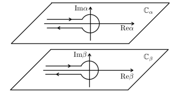
Figure 6: The Hankel path of integration.

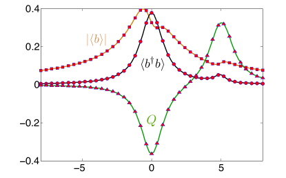
Figure 7: (Color online) Comparison of the numerical steady state solution of $|\langle b\rangle|$, $\langle b^{\dagger}b\rangle$ and $Q$ under the original master equation for bosonization model (solid lines) with the analytical results Eqs. (28)-(30) (markers) in the main text. All parameters are the same as in figure 2(b).

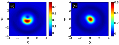
Figure 8: (Color online) Wigner function $W(x,p)$ of the quantum mechanical steady-state solution with (a) $\Delta=0$ and (b) $\Delta=\chi/2$.

The generalized $P(\alpha,\beta)$ function has to satisfying the normalization condition, which implies

$$I = \int^{(\mathbb{C}_{\alpha},\mathbb{C}_{\beta})}P_{ss}(\alpha,\beta)d\alpha d\beta$$

$$= \int^{(\mathbb{C}_{\alpha},\mathbb{C}_{\beta})}d\alpha d\beta\alpha^{c-2}\beta^{d-2}e^{-z(1/\alpha+1/\beta)+2\alpha\beta}$$

$$= \int^{(\mathbb{C}_{\alpha},\mathbb{C}_{\beta})}d(\alpha^{-1})d(\beta^{-1})\sum_{n=0}^{\infty}\frac{2^{n}}{n!}\alpha^{c+n}\beta^{d+n}e^{-z(1/\alpha+1/\beta)}$$

$$= \int^{(\mathbb{C}_{\alpha},\mathbb{C}_{\beta})}d\alpha_{1}d\beta_{1}\sum_{n=0}^{\infty}\frac{2^{n}}{n!}\alpha_{1}^{-(c+n)}\beta_{1}^{-(d+n)}e^{-z(\alpha_{1}+\beta_{1})}$$

with $\alpha_{1}=\alpha^{-1}$ and $\beta_{1}=\beta^{-1}$. On the other hand, the Gamma-function identity can be defined by using the Hankel path of integration $\mathcal{O}$ (see Fig. 6)

$$\frac{1}{\Gamma(c+n)} = \frac{1}{2\pi i}\int_{\mathcal{O}}(\sigma z)^{-(c+n)}e^{\sigma z}d(\sigma z)$$ (58)

$$= \frac{z{}^{1-(c+n)}}{2\pi i}\int_{\mathcal{O}}\sigma{}^{-(c+n)}e^{\sigma z}d\sigma,$$

with which we obtain

$$I = \int^{(\mathbb{C}_{\alpha},\mathbb{C}_{\beta})}d\alpha_{1}d\beta_{1}\sum_{n=0}^{\infty}\frac{2^{n}}{n!}\alpha_{1}^{-(c+n)}\beta_{1}^{-(d+n)}e^{-z(\alpha_{1}+\beta_{1})}$$ (59)

$$= \sum_{n=0}^{\infty}\frac{2^{n}}{n!}[\int_{\mathcal{O}}d\alpha_{1}\alpha_{1}^{-(c+n)}e^{-z\alpha_{1}}\int_{\mathcal{O}}d\beta_{1}\beta_{1}^{-(d+n)}e^{-z\beta_{1}}]$$

$$= (-4\pi^{2})\sum_{n=0}^{\infty}\frac{2^{n}}{n!}\frac{z{}^{c+d+2(n-1)}}{\Gamma(c+n)\Gamma(d+n)}$$

$$= \frac{(-4\pi^{2})z{}^{c+d-2}}{\Gamma(c)\Gamma(d)}{}_{0}F_{2}(c,d,2z^{2}),$$

where ${}_{0}F_{2}(c,d,z)$ is the generalized hypergeometric function defined as

$${}_{0}F_{2}(c,d,z)=\sum_{n=0}^{\infty}\frac{z^{n}}{n!}\frac{\Gamma(c)\Gamma(d)}{\Gamma(c+n)\Gamma(d+n)}.$$ (60)

The normalized $i$th-order correlation function $G^{(i,j)}$ corresponding to the normally ordered averages $\langle b^{\dagger i}b^{j}\rangle$ can be calculated by the generalized $P$-representation:

$$G^{(i,j)} = \frac{\int d\sigma(\alpha,\beta)P(\alpha,\beta)\beta^{m}\alpha^{n}}{\int d\sigma(\alpha,\beta)P(\alpha,\beta)}$$

$$= \frac{\frac{(-4\pi^{2})z{}^{c+d-2+i+j}}{\Gamma(c+j)\Gamma(d+i)}{}_{0}F_{2}(c+j,d+i,2z^{2})}{\frac{(-4\pi^{2})z{}^{c+d-2}}{\Gamma(c)\Gamma(d)}{}_{0}F_{2}(c,d,2z^{2})}.$$

With the Euler’s functional equation $\Gamma(z)/\Gamma(z+n+1)=1/z(z+1)\cdots(z+n)$, we finally have

$$G^{(i,j)}=z{}^{i+j}\frac{\Gamma(c)\Gamma(d){}_{0}F_{2}(c+j,d+i,2z^{2})}{\Gamma(c+j)\Gamma(d+i){}_{0}F_{2}(c,d,2z^{2})},$$ (62)

and therefore the quantum mechanical steady-state solution of $\langle b\rangle$, $\langle b^{\dagger}b\rangle$ and $Q=\frac{\langle b^{\dagger}b^{\dagger}bb\rangle}{\langle b^{\dagger}b\rangle}-\langle b^{\dagger}b\rangle$. We have verified these analytical results by comparisons with the numerically obtained steady state solution of the original master equation $\dot{\rho}=-i[H_{b},\rho]+\frac{\gamma}{2}(2b\rho b^{\dagger}-\rho b^{\dagger}b-b^{\dagger}b\rho)$. And as shown in figure 7, we find excellent agreement between the two different ways.

Appendix D The nonclassical nature of the quantum mechanical steady states

The nonclassical nature of the quantum mechanical steady states for the excitation processes with resonant driving and the laser detuning $\Delta=\chi/2$ manifests itself in the Wigner function with negative value, as shown in figure 8.

References

- Saffman et al. (2010) M. Saffman, T. G. Walker, and K. Mølmer, Rev. Mod. Phys. 82, 2313 (2010).
- Chang et al. (2014) D. E. Chang, V. Vuletić, and M. D. Lukin, Nat. Photon. 8, 685 (2014).
- Pritchard et al. (2010) J. D. Pritchard, D. Maxwell, A. Gauguet, K. J. Weatherill, M. P. A. Jones, and C. S. Adams, Phys. Rev. Lett. 105, 193603 (2010).
- Sevinçli et al. (2011) S. Sevinçli, N. Henkel, C. Ates, and T. Pohl, Phys. Rev. Lett. 107, 153001 (2011).
- Petrosyan et al. (2011) D. Petrosyan, J. Otterbach, and M. Fleischhauer, Phys. Rev. Lett. 107, 213601 (2011).
- Peyronel et al. (2012) T. Peyronel, O. Firstenberg, Q.-Y. Liang, S. Hofferberth, A. V. Gorshkov, T. Pohl, M. D. Lukin, and V. Vuletić, Nature (London) 488, 57 (2012).
- Parigi et al. (2012) V. Parigi, E. Bimbard, J. Stanojevic, A. J. Hilliard, F. Nogrette, R. Tualle-Brouri, A. Ourjoumtsev, and P. Grangier, Phys. Rev. Lett. 109, 233602 (2012).
- Yan et al. (2012) D. Yan, Y.-M. Liu, Q.-Q. Bao, C.-B. Fu, and J.-H. Wu, Phys. Rev. A 86, 023828 (2012).
- Gorshkov et al. (2013) A. V. Gorshkov, R. Nath, and T. Pohl, Phys. Rev. Lett. 110, 153601 (2013).
- Maxwell et al. (2013) D. Maxwell, D. J. Szwer, D. Paredes-Barato, H. Busche, J. D. Pritchard, A. Gauguet, K. J. Weatherill, M. P. A. Jones, and C. S. Adams, Phys. Rev. Lett. 110, 103001 (2013).
- He et al. (2014) B. He, A. V. Sharypov, J. Sheng, C. Simon, and M. Xiao, Phys. Rev. Lett. 112, 133606 (2014).
- Li et al. (2014) W. Li, D. Viscor, S. Hofferberth, and I. Lesanovsky, Phys. Rev. Lett. 112, 243601 (2014).
- Maghrebi et al. (2015) M. F. Maghrebi, M. J. Gullans, P. Bienias, S. Choi, I. Martin, O. Firstenberg, M. D. Lukin, H. P. Büchler, and a. V. Gorshkov, Phys. Rev. Lett 115, 123601 (2015).
- Weimer et al. (2008) H. Weimer, R. Löw, T. Pfau, and H. P. Büchler, Phys. Rev. Lett. 101, 250601 (2008).
- Weimer and Büchler (2010) H. Weimer and H. P. Büchler, Phys. Rev. Lett. 105, 230403 (2010).
- Lee et al. (2011) T. E. Lee, H. Häffner, and M. C. Cross, Phys. Rev. A 84, 031402 (2011).
- Qian et al. (2012) J. Qian, G. Dong, L. Zhou, and W. Zhang, Phys. Rev. A 85, 065401 (2012).
- Lesanovsky and Garrahan (2013) I. Lesanovsky and J. P. Garrahan, Phys. Rev. Lett. 111, 215305 (2013).
- Marcuzzi et al. (2014) M. Marcuzzi, E. Levi, S. Diehl, J. P. Garrahan, and I. Lesanovsky, Phys. Rev. Lett. 113, 210401 (2014).
- Hoening et al. (2014) M. Hoening, W. Abdussalam, M. Fleischhauer, and T. Pohl, Phys. Rev. A 90, 021603 (2014).
- Glaetzle et al. (2012) A. W. Glaetzle, R. Nath, B. Zhao, G. Pupillo, and P. Zoller, Phys. Rev. A 86, 043403 (2012).
- Höning et al. (2013) M. Höning, D. Muth, D. Petrosyan, and M. Fleischhauer, Phys. Rev. A 87, 023401 (2013).
- Vermersch et al. (2015) B. Vermersch, M. Punk, a. W. Glaetzle, C. Gross, and P. Zoller, New J. Phys. 17, 013008 (2015).
- Ates et al. (2007a) C. Ates, T. Pohl, T. Pattard, and J. M. Rost, Phys. Rev. Lett. 98, 023002 (2007).
- Ates et al. (2007b) C. Ates, T. Pohl, T. Pattard, and J. Rost, Phys. Rev. A 76, 013413 (2007).
- Mayle et al. (2011) M. Mayle, W. Zeller, N. Tezak, and P. Schmelcher, Phys. Rev. A 84, 010701 (2011).
- Ates and Lesanovsky (2012) C. Ates and I. Lesanovsky, Phys. Rev. A 86, 013408 (2012).
- Petrosyan et al. (2013) D. Petrosyan, M. Höning, and M. Fleischhauer, Phys. Rev. A 87, 053414 (2013).
- Gärttner et al. (2013) M. Gärttner, K. P. Heeg, T. Gasenzer, and J. Evers, Phys. Rev. A 88, 043410 (2013).
- Bettelli et al. (2013) S. Bettelli, D. Maxwell, T. Fernholz, C. S. Adams, I. Lesanovsky, and C. Ates, Phys. Rev. A 88, 043436 (2013).
- Sanders et al. (2015) J. Sanders, M. Jonckheere, and S. Kokkelmans, Phys. Rev. Lett. 115, 043002 (2015).
- Ates et al. (2012) C. Ates, B. Olmos, J. P. Garrahan, and I. Lesanovsky, Phys. Rev. A 85, 043620 (2012).
- Lee and Cross (2012) T. E. Lee and M. C. Cross, Phys. Rev. A 85, 063822 (2012).
- Lee et al. (2012) T. E. Lee, H. Häffner, and M. C. Cross, Phys. Rev. Lett. 108, 023602 (2012).
- Hu et al. (2013) A. Hu, T. E. Lee, and C. W. Clark, Phys. Rev. A 88, 053627 (2013).
- Schönleber et al. (2014) D. W. Schönleber, M. Gärttner, and J. Evers, Phys. Rev. A 89, 033421 (2014).
- Gärttner et al. (2014) M. Gärttner, S. Whitlock, D. W. Schönleber, and J. Evers, Phys. Rev. Lett. 113, 233002 (2014).
- Olmos et al. (2014) B. Olmos, D. Yu, and I. Lesanovsky, Phys. Rev. A 89, 023616 (2014).
- Weimer (2015) H. Weimer, Phys. Rev. A 91, 063401 (2015).
- Schempp et al. (2015) H. Schempp, G. Günter, S. Wüster, M. Weidemüller, and S. Whitlock, Phys. Rev. Lett. 115, 093002 (2015).
- Viteau et al. (2012) M. Viteau, P. Huillery, M. G. Bason, N. Malossi, D. Ciampini, O. Morsch, E. Arimondo, D. Comparat, and P. Pillet, Phys. Rev. Lett. 109, 053002 (2012).
- Hofmann et al. (2013) C. S. Hofmann, G. Günter, H. Schempp, M. Robert-de Saint-Vincent, M. Gärttner, J. Evers, S. Whitlock, and M. Weidemüller, Phys. Rev. Lett. 110, 203601 (2013).
- Carr et al. (2013) C. Carr, R. Ritter, C. G. Wade, C. S. Adams, and K. J. Weatherill, Phys. Rev. Lett. 111, 113901 (2013).
- Schempp et al. (2014) H. Schempp, G. Günter, M. Robert-de Saint-Vincent, C. S. Hofmann, D. Breyel, A. Komnik, D. W. Schönleber, M. Gärttner, J. Evers, S. Whitlock, et al., Phys. Rev. Lett. 112, 013002 (2014).
- Urvoy et al. (2015) A. Urvoy, F. Ripka, I. Lesanovsky, D. Booth, J. P. Shaffer, T. Pfau, and R. Löw, Phys. Rev. Lett. 114, 203002 (2015).
- Malossi et al. (2014) N. Malossi, M. M. Valado, S. Scotto, P. Huillery, P. Pillet, D. Ciampini, E. Arimondo, and O. Morsch, Phys. Rev. Lett. 113, 023006 (2014).
- Valado et al. (2015) M. M. Valado, C. Simonelli, M. D. Hoogerland, I. Lesanovsky, J. P. Garrahan, E. Arimondo, D. Ciampini, O. Morsch, and F. E. Fermi, Phys. Rev. A 93, 040701(R) (2016).
- Günter et al. (2012) G. Günter, M. Robert-de Saint-Vincent, H. Schempp, C. S. Hofmann, S. Whitlock, and M. Weidemüller, Phys. Rev. Lett. 108, 013002 (2012).
- Schwarzkopf et al. (2011) A. Schwarzkopf, R. E. Sapiro, and G. Raithel, Phys. Rev. Lett. 107, 103001 (2011).
- Drummond and Walls (1980) P. D. Drummond and D. F. Walls, Journal of Physics A: Mathematical and General 13, 725 (1980).
- Labuhn et al. (2016) H. Labuhn, D. Barredo, S. Ravets, S. de Léséleuc, T. Macrì, T. Lahaye, and A. Browaeys, Nature(London) 534, 667 (2016).
- Britton et al. (2012) J. W. Britton, B. C. Sawyer, A. C. Keith, C. C. J. Wang, J. K. Freericks, H. Uys, M. J. Biercuk, and J. J. Bollinger, Nature(London) 484, 489 (2012).
- Sun et al. (2003) C. P. Sun, Y. Li, and X. F. Liu, Phys. Rev. Lett. 91, 147903 (2003).
- Hammerer et al. (2010) K. Hammerer, A. S. Sørensen, and E. S. Polzik, Rev. Mod. Phys. 82, 1041 (2010).
- Wüster et al. (2010) S. Wüster, J. Stanojevic, C. Ates, T. Pohl, P. Deuar, J. F. Corney, and J. M. Rost, Phys. Rev. A 81, 023406 (2010).
- Haken (1975) H. Haken, Rev. Mod. Phys. 47, 67 (1975).