The Limiting Dynamics of a Bistable Molecular Switch With and Without Noise

Abstract

We consider the dynamics of a population of organisms containing two mutually inhibitory gene regulatory networks, that can result in a bistable switch-like behaviour. We completely characterize their local and global dynamics in the absence of any noise, and then go on to consider the effects of either noise coming from bursting (transcription or translation), or Gaussian noise in molecular degradation rates when there is a dominant slow variable in the system. We show analytically how the steady state distribution in the population can range from a single unimodal distribution through a bimodal distribution and give the explicit analytic form for the invariant stationary density which is globally asymptotically stable. Rather remarkably, the behaviour of the stationary density with respect to the parameters characterizing the molecular behaviour of the bistable switch is qualitatively identical in the presence of noise coming from bursting as well as in the presence of Gaussian noise in the degradation rate. This implies that one cannot distinguish between either the dominant source or nature of noise based on the stationary molecular distribution in a population of cells. We finally show that the switch model with bursting but two dominant slow genes has an asymptotically stable stationary density.

1 Introduction

In electrical circuits there are only two elementary ways to produce bistable behavior. Either with positive feedback (e.g. A stimulates B and B stimulates A) or with double negative feedback (A inhibits B and B inhibits A). This elementary fact, known to all electrical engineering students, has, in recent years, come to the attention of molecular biologists who have rushed to implicate one or the other mechanism as the source of putative or real bistable behavior in a variety of biological systems. (In a gene regulatory framework we might term the double positive feedback switch an inducible switch, while the double negative feedback switch could be called a repressible switch.) Some laboratories have used this insight to engineer in vitro systems to have bistable behavior and one of the first was Gardner et al (2000) who engineered repressible switch like behavior of the type we study in this paper. Some especially well written surveys are to be found in Ferrell (2002), Tyson et al (2003), and Angeli et al (2004).

Gene regulatory networks are, however, noisy affairs for a variety of reasons and it is now thought that this noise may actually play a significant role in determining function (Eldar and Elowitz, 2010). In such noisy dynamical systems experimentalists will often take a populational level approach and infer the existence of underlying bistable behavior based on the existence of bimodal densities of some molecular constituent over some range of experimental parameter values.

From a modeling perspective there have been a number of studies attempting to understand the effects of noise on gene regulatory dynamics. The now classical Kepler and Elston (2001) really laid much of the ground work for subsequent studies by its treatment of a variety of noise sources and their effect on dynamics. Mackey et al (2011) examined the effects of either bursting or Gaussian noise on both inducible and repressible operon models, and Waldherr et al (2010) looked at the role of Gaussian noise in an inducible switch model for ovarian follicular growth.

One of the most interesting situations is the observation that the presence of noise may induce bistability in a gene regulatory model when it was absolutely impossible to have bistable behaviour in the absence of noise. This has been very nicely explored by Artyomov et al (2007) (in competing positive/negative feedback motifs), and Samoilov et al (2005) (in enzymatic futile cycles), while Qian et al (2009) and Bishop and Qian (2010) analytically explored noise induced bistability, the latter in a phosphorylation-dephosphorylation cycle model. Vellela and Qian (2009) examined the role of noise in shaping the dynamics of the bistable Schlögl chemical kinetic model.

For bistable repressible switch models Wang et al (2007) examined quorum-sensing with degradation rate noise in phage $\Lambda$ while Morelli et al (2008a) examined the role of noise in protein production rates. Morelli et al (2008b) carried out numerical studies of repressible switch slow dynamics in the face of noise. Bokes et al (2013) gave a nice overview of the various approaches to the modeling of these systems and then examined the role of transcriptional/translational bursting in repressible and inducible systems as well as in a repressible switch. Caravagna et al (2013) examined the effects of bounded Gaussian noise on mRNA production rates in a repressible switch model, while Strasser et al (2012) have looked at a model for the Pu/Gata switch (a repressible switch implicated in hematopoietic differentiation decision making) with high levels of protein and low levels of DNA.

In this paper, we extend the work of Mackey et al (2011) on inducible and repressible systems to an analytic consideration of an inducible switch in the presence of either bursting transcriptional (or translational) noise or Gaussian noise. The paper is organized as follows. Section 2 lays the groundwork by developing the deterministic model based on ordinary differential equations (a generalization of Grigorov et al (1967), the earliest study we know of, and Cherry and Adler (2000)) that we use to consider the influence of noise. This is followed in Section 3 with an analysis of the deterministic system, including the coexistence of multiple steady states, and their stability. This section, though superficially similar to the treatment of Mackey et al (2011), extends their results to a completely different situation than previously considered, namely a model for a repressible switch. Section 4 briefly considers how the existence of fast and slow variables enables the simplification of the dynamics, and consequently makes computations tractable, while the following Section 5 introduces bursting transcriptional or translational noise and derives the stationary population density in a variety of situations when there is a single dominant slow variable. We not only give explicit analytic expressions for these stationary densities, but also show that they are globally asymptotically stable. Section 6 considers an alternative situation in which there is Gaussian distributed noise in the degradation rate for a single slow variable. We again give the analytic form for the stationary densities as well as demonstrating their stability. Section 7 expands on Section 5 by considering bursting transcription or translation but in the situation where there are two dominant slow variables. The models in Sections 5-7 are expressed as stochastic differential equations. The paper concludes with a short discussion.

2 The bistable genetic switch

2.1 Biological background

The paradigmatic molecular biology example of a bistable switch due to reciprocal negative feedback is the bacteriophage (or phage) $\lambda$, which is a virus capable of infecting Escherichia coli bacteria. Originally described in Jacob and Monod (1961) and very nicely treated in Ptashne (1986), it is but one of scores of mutually inhibitory bistable switches that have been found since.

2.2 Model development

Figure 1 gives a cartoon representation of the situation we are modeling here, which is a generalization of the work of Grigorov et al (1967) and Cherry and Adler (2000). The original postulate for the hypothetical regulatory network of Figure 1 is to be found in the lovely paper (Monod and Jacob, 1961) which treats a number of different molecular control scenarios, and the reader may find reference to that figure helpful while following the model development below. It should be noted that with the advent of the power of synthetic biology it is now possible to construct molecular control circuits with virtually any desired configuration and thereby experimentally investigate their dynamics (Hasty et al, 2001).

Figure 1: A schematic depiction of the elements of a bistable genetic switch, following Monod and Jacob (1961). There are two operons ($X$ and $Y$). For each, the regulatory region ($Reg_{x}$ or $Reg_{y}$) produces a repressor molecule ($R_{x}$ or $R_{y}$) that is inactive unless it is combined with the effector produced by the opposing operon ($E_{y}$ or $E_{x}$ respectively). In the combined form ($R_{x}E_{y}$ or $R_{y}E_{x}$) the repressor-effector complex binds to the operator region ($O_{x}$ or $O_{y}$ respectively) and blocks transcription of the corresponding structural gene ($SG_{x}$ or $SG_{y}$). When the operator region is not complexed with the active form of the repressor, transcription of the structural gene can take place and mRNA ($M_{x}$ or $M_{y}$) is produced. Translation of the mRNA then produces an effector molecule ($E_{x}$ or $E_{y}$). These effector molecules then are capable of interacting with the repressor molecule of the opposing gene. See Monod and Jacob (1961).

Polynikis et al (2009) offers a nice survey of techniques applicable to the approach we take in this section. We consider two operons $X$ and $Y$ such that the ‘effector’ of $X$, denoted by $E_{x}$, inhibits the transcriptional production of mRNA from operon $Y$ and vice versa. We take the approach of Goodwin (1965) as extended and developed in (Griffith, 1968a, b; Othmer, 1976; Selgrade, 1979). Consider initially a single operon $a$ where $a\in\{x,y\}$ and denote by $\bar{a}\in\{y,x\}$ the opposing operon. For the mutually repressible systems we consider here, in the presence of the effector molecule $E_{a}$ the repressor $R_{\bar{a}}$ is active (able to bind to the operator region), and thus block DNA transcription. The effector binds with the inactive form $R_{\bar{a}}$ of the repressor, and when bound to the effector the repressor becomes active. We take this reaction to be in equilibrium and of the form

$$R_{\bar{a}}+n_{\bar{a}}E_{a}\rightleftharpoons R_{\bar{a}}E_{an_{\bar{a}}}.$$ (1)

Here, $R_{\bar{a}}E_{an_{\bar{a}}}$ is a repressor-effector complex and $n_{\bar{a}}$ is the number of effector molecules that inactivate the repressor $R_{\bar{a}}$. If we let the mRNA and effector concentrations be denoted by $(M_{a},E_{a})$ then we assume that the dynamics for operon $a$ are given by

$$\dfrac{dM_{a}}{dt} =\bar{b}_{d,a}\bar{\varphi}_{m,a}f_{a}(E_{\bar{a}})-\gamma_{M_{a}}M_{a},\quad\bar{a}\in\{y,x\}$$ (2)

$$\dfrac{dE_{a}}{dt} =\beta_{E_{a}}M_{a}-\gamma_{E_{a}}E_{a}.$$ (3)

It is assumed in (2) that the rate of mRNA production is proportional to the fraction of time the operator region is active and that the maximum level of transcription is $\bar{b}_{d,a}$, and that the effector production rate is proportional to the amount of mRNA. Note that the production of $M_{x}$ is regulated by $E_{y}$ and vice versa, and that the components $(M_{a},E_{a})$ are subject to degradation. The function $f$ is calculated next.

To compute $f$ we temporarily suppress the subscript $a$ and then restore it at the end. Let the corresponding reaction in (1) and the equilibrium constant be

$$R+nE\stackrel{{\scriptstyle K_{1}}}{{\rightleftharpoons}}RE_{n}\qquad K_{1}=\frac{RE_{n}}{R\cdot E^{n}}.$$

There is an interaction between the operator $O$ and repressor $R$ described by

$$O+RE_{n}\stackrel{{\scriptstyle K_{2}}}{{\rightleftharpoons}}ORE_{n}\qquad K_{2}=\frac{ORE_{n}}{O\cdot RE_{n}}.$$

The total operator is given by

$$O_{tot}=O+ORE_{n}=O+K_{1}K_{2}O\cdot R\cdot E^{n}=O(1+K_{1}K_{2}R\cdot E^{n}),$$

while the total repressor $R_{tot}$ is

$$R_{tot}=R+K_{1}R\cdot E^{n}+K_{2}O\cdot RE_{n},$$

so the fraction of operators not bound by repressor is given by

$$f(E)=\frac{O}{O_{tot}}=\frac{1}{1+K_{1}K_{2}R\cdot E^{n}}.$$

If the amount repressor bound to the operator is small compared to the total amount of repressor then $R_{tot}\simeq R(1+K_{1}\cdot E^{n})$ and consequently

$$f(E)=\frac{1+K_{1}E^{n}}{1+(K_{1}+K_{1}K_{2}R_{tot})E^{n}}=\frac{1+K_{1}E^{n}}{1+KE^{n}},$$

where $K=K_{1}(1+K_{2}R_{tot})$. When $E$ is large there will be maximal repression, but even then there will still be a basal level of mRNA production proportional to $K_{1}K^{-1}<1$ (this is known as leakage). The variation of the DNA transcription rate with effector level is given by $\varphi=\bar{\varphi}_{m}f$ or

$$\varphi(E)=\bar{\varphi}_{m}\frac{1+K_{1}E^{n}}{1+KE^{n}}=\bar{\varphi}_{m}f(E),$$ (4)

where $\bar{\varphi}_{m}$ is the maximal DNA transcription rate (in units of inverse time).

Now explicitly including the proper subscripts we have

$$\varphi_{a}(E_{\bar{a}})=\bar{\varphi}_{m,a}\frac{1+K_{1,a}E_{\bar{a}}^{n_{a}}}{1+K_{a}E_{\bar{a}}^{n_{a}}}=\bar{\varphi}_{m,a}f_{a}(E_{\bar{a}}),$$

where $K_{a}=K_{1,a}(1+K_{2,a}R_{tot,a})$.

We next rewrite Equations 2-3 by defining dimensionless concentrations. Equation 4 becomes

$$\varphi_{a}(e_{\bar{a}})=\varphi_{m,a}f_{a}(e_{\bar{a}}),$$

where the dimensionless rate $\varphi_{m,a}$ is defined by

$$\varphi_{m,a}=\dfrac{\bar{\varphi}_{m,a}\beta_{E,a}}{\gamma_{M,a}\gamma_{E,a}}\quad\mbox{and}\quad f_{a}(e_{\bar{a}})=\dfrac{1+e_{\bar{a}}^{n_{a}}}{1+\Delta_{a}e_{\bar{a}}^{n_{a}}},$$

$\Delta_{a}=K_{a}K_{1,a}^{-1}$, and the dimensionless effector concentration $(e_{a})$ is defined by

$$E_{a}=\eta_{a}e_{\bar{a}}\quad\mbox{with}\quad\eta_{a}=\dfrac{1}{\sqrt[n_{a}]{K_{1,a}}}.$$

Recall that $\Delta_{a}^{-1}$ denotes the leakage and note that if $\Delta_{a}$ goes to infinity then the transcription goes to zero. Similarly using a dimensionless mRNA concentration ($m_{a}$) given by

$$M_{a}=m_{a}\eta_{a}\dfrac{\gamma_{E_{a}}}{\beta_{E_{a}}},$$

Equations 2-3 take the form

$$\dfrac{dm_{a}}{dt} =\gamma_{M_{a}}[\kappa_{d,a}f_{a}(e_{\bar{a}})-m_{a}],$$

$$\dfrac{de_{a}}{dt} =\gamma_{E_{a}}(m_{a}-e_{a}),$$

with

$$\kappa_{d,a}=b_{d,a}\varphi_{m,a},\quad\mbox{and}\quad b_{d,a}=\dfrac{\bar{b}_{d,a}}{\eta_{a}}$$

which are both dimensionless.

Thus the equations governing the dynamics of this system are given by the four differential equations

$$\dfrac{dm_{x}}{dt} =\gamma_{M_{x}}[\kappa_{d,x}f_{x}(e_{y})-m_{x}],$$

$$\dfrac{de_{x}}{dt} =\gamma_{E_{x}}(m_{x}-e_{x}),$$

$$\dfrac{dm_{y}}{dt} =\gamma_{M_{y}}[\kappa_{d,y}f_{y}(e_{x})-m_{y}],$$

$$\dfrac{de_{y}}{dt} =\gamma_{E_{y}}(m_{y}-e_{y})$$

where

$$f_{x}(e_{y})=\dfrac{1+e_{y}^{n_{x}}}{1+\Delta_{x}e_{y}^{n_{x}}}\quad\mbox{and}\quad f_{y}(e_{x})=\dfrac{1+e_{x}^{n_{y}}}{1+\Delta_{y}e_{x}^{n_{y}}}.$$

To make the model equations somewhat more straightforward, denote dimensionless concentrations by $(m_{x},e_{x},m_{y},e_{y})=(x_{1},x_{2},y_{1},y_{2})$ (with obvious changes in the other subscripts) to obtain

$$\dfrac{dx_{1}}{dt} =\gamma_{x_{1}}[\kappa_{d,x}f_{x}(y_{2})-x_{1}],$$ (5)

$$\dfrac{dx_{2}}{dt} =\gamma_{x_{2}}(x_{1}-x_{2}),$$ (6)

$$\dfrac{dy_{1}}{dt} =\gamma_{y_{1}}[\kappa_{d,y}f_{y}(x_{2})-y_{1}],$$ (7)

$$\dfrac{dy_{2}}{dt} =\gamma_{y_{2}}(y_{1}-y_{2}),$$ (8)

Throughout, $\gamma_{\cdot}$ is a decay rate (time^-1), and so Equations 5-8 are not dimensionless. In addition to the loss rates explicitly appearing, we have the parameters $\kappa_{d,x},\kappa_{d,y}$. Since

$$f_{x}(y_{2})=\dfrac{1+y_{2}^{n_{x}}}{1+\Delta_{x}y_{2}^{n_{x}}}\quad\mbox{and}\quad f_{y}(x_{2})=\dfrac{1+x_{2}^{n_{y}}}{1+\Delta_{y}x_{2}^{n_{y}}},$$ (9)

we have as well the four parameters $\Delta_{x},\Delta_{y},n_{x},n_{y}$ to consider. Note that

$$f_{x}(0)=1,\,\lim_{y_{2}\to\infty}f_{x}(y_{2})=\Delta_{x}^{-1}<1,\,f_{y}(0)=1,\,\lim_{x_{2}\to\infty}f_{y}(x_{2})=\Delta_{y}^{-1}<1.$$

3 Steady states and dynamics

The dynamics of this model for a bistable switch can be analyzed as follows. This section is an elaboration of aspects of the work presented in Cherry and Adler (2000). Set $W=(x_{1},x_{2},y_{1},y_{2})$ so the system (5)-(8) generates a flow $S_{t}(W)$. The flow $S_{t}(W^{0})\in\mathbb{R}_{4}^{+}$ for all initial conditions $W^{0}=(x_{1}^{0},x_{2}^{0},,y_{1}^{0},y_{2}^{0})\in\mathbb{R}_{4}^{+}$ and $t>0$.

The steady states of the system (5)-(8) are given by $x_{1}^{*}=x_{2}^{*}=x^{*},y_{1}^{*}=y_{2}^{*}=y^{*}$ where $(x^{*},y^{*})$ is the solution of

$$x_{1} =x_{2}=\kappa_{d,x}f_{x}(y_{2})$$ (10)

$$y_{1} =y_{2}=\kappa_{d,y}f_{y}(x_{2}).$$ (11)

For each solution $(x^{*},y^{*})$ of (10)-(11) there is a steady state $W^{*}$ of the model, and the parameters $(\kappa_{d,x},\kappa_{d,y},\Delta_{x},\Delta_{y},n_{x},n_{y})$ will determine whether $W^{*}$ is unique or has multiple values.

3.1 Graphical investigation of the steady states

Figure 2 gives a graphical picture of the five qualitative possibilities for steady state solutions of the pair of equations (5)-(8).

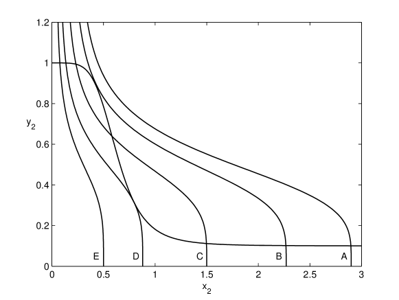
Figure 2: A graphical representation of the possible steady state solutions of Equations 10 and 11. We have plotted the $y_{1}$ and $x_{1}$ isoclines ($y_{2}=\kappa_{d,y}f_{y}(x_{2})$ and $x_{2}=\kappa_{d,x}f_{x}(y_{2})$ respectively), and assumed that the $y_{1}$ isocline (the graph of $y_{2}=\kappa_{d,y}f_{y}(x_{2})$) is not changed but that $x_{1}$ isocline (the graph of $x_{2}=\kappa_{d,x}f_{x}(y_{2})$) is varied as indicated by the labels A to E, e.g. by decreasing $\kappa_{d,x}$. (A) There is a single steady state at a large value of $x_{2}$ and a correspondingly small value of $y_{2}$. In this case operon $X$ of the bistable switch is in the “ON” state while operon $Y$ is in the “OFF” state. This steady state is globally stable. (B) A decrease in $\kappa_{d,x}$ now leads to a situation in which there are two steady states, the largest (locally stable one) corresponding to the intersection of the two graphs, and the second smaller (half stable) one where the two graphs are tangent. (C) Further decreases in $\kappa_{d,x}$ now result in three steady states. For the largest (locally stable) one the operon $X$ is in the on state while $Y$ is in the off state. The smallest one (also locally stable) corresponds to operon $Y$ in the ON state and $X$ is in the OFF state. The intermediate steady state is unstable. (D) This case is like B in that there are two steady states, one (locally stable) defined by the intersection of the two graphs in which $Y$ is ON and the second at the tangency of the two graphs is again half stable. (E) Finally, for sufficiently small $\kappa_{d,x}$ there is a single globally stable steady state in which $Y$ is ON and $X$ is OFF.

An alternative, but equivalent, way of examining the steady state of this model is by examining the solution of either one of the pair of equations

$$\dfrac{x}{\kappa_{d,x}}=f_{x}(\kappa_{d,y}f_{y}(x)):={\mathcal{F}}_{x}(x),\,\,\dfrac{y}{\kappa_{d,y}}=f_{y}(\kappa_{d,x}f_{x}(y)):={\mathcal{F}}_{y}(y).$$

We choose to deal with the first. Note that since both $f_{x}$ and $f_{y}$ are monotone decreasing functions of their arguments, the composition of the two

$${\mathcal{F}}_{x}(x)=\dfrac{1+(\kappa_{d,y}f_{y}(x))^{n_{x}}}{1+\Delta_{x}(\kappa_{d,y}f_{y}(x))^{n_{x}}}=\dfrac{1+\left(\kappa_{d,y}\dfrac{1+x^{n_{y}}}{1+\Delta_{y}x^{n_{y}}}\right)^{n_{x}}}{1+\Delta_{x}\left(\kappa_{d,y}\dfrac{1+x^{n_{y}}}{1+\Delta_{y}x^{n_{y}}}\right)^{n_{x}}}$$ (12)

is a monotone increasing function of $x$ with

$${\mathcal{F}}_{x}(0)=\dfrac{1+\kappa_{d,y}^{n_{x}}}{1+\Delta_{x}\kappa_{d,y}^{n_{x}}}:={\mathcal{F}}_{x,0}$$

and

$$\lim_{x\to\infty}{\mathcal{F}}_{x}(x)=\dfrac{1+(\kappa_{d,y}\Delta_{y}^{-1})^{n_{x}}}{1+\Delta_{x}(\kappa_{d,y}\Delta_{y}^{-1})^{n_{x}}}:={\mathcal{F}}_{x,\infty}>{\mathcal{F}}_{x,0}.$$

In Figure 3 we have shown graphically the same sequence of steady states as we illustrated in Figure 2

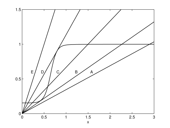
Figure 3: A graphical representation of the possible steady state solutions of the equation ${x}/{\kappa_{d,x}}=f_{x}(\kappa_{d,y}f_{y}(x)):={\mathcal{F}}_{x}(x)$. The smooth monotone increasing graph is that of ${\mathcal{F}}_{x}(x)$ as given in Equation 12, while the straight line is that of ${x}/{\kappa_{d,x}}$ for different values of $\kappa_{d,x}$. The five straight lines correspond to the five possibilities (A through E) in Figure 2.

3.2 Analytic investigation of the steady states

Single versus multiple steady states. This model for a bistable genetic switch may have one [$W_{1}^{*}$ ( E of Figure 2 or Figure 3) or $W_{3}^{*}$ (A)], two [$W_{1}^{*},W_{2}^{*}=W_{3}^{*}$ (D) or $W_{1}^{*}=W_{2}^{*},W_{3}^{*}$ (B)], or three [$W_{1}^{*},W_{2}^{*},W_{3}^{*}$ (C)] steady states, with the ordering $0\preceq W_{1}^{*}\preceq W_{2}^{*}\preceq W_{3}^{*}$, indicating that $W_{1}^{*}$ corresponds to operon $X$ in the OFF state and operon $Y$ in the ON state while at $W_{3}^{*}$ $X$ is ON and $Y$ is OFF.

Analytic conditions for the existence of one or more steady states can be obtained by first noting that we must have

$$\dfrac{x}{\kappa_{d,x}}=f_{x}(\kappa_{d,y}f_{y}(x)):={\mathcal{F}}_{x}(x)$$ (13)

satisfied. In Figure 4 we have illustrated Equation 13 for various values of parameters.

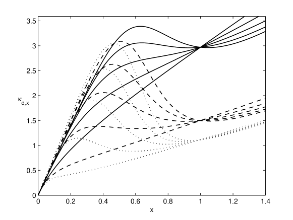
Figure 4: The plot of $\kappa_{d,x}$ versus $x$ obtained from Equation 13. The figure was constructed for the following parameters: $n_{x}\in\{1,2,3\}$, $n_{y}\in\{1,2,3,4,5\}$, $\kappa_{y}=2$, $\Delta_{x}=12$, $\Delta_{y}=10$. The solid lines correspond to $n_{x}=1$ and we increase $n_{y}$ from $1$ (the lowest line) to $5$ (the top one). The dashed lines correspond to $n_{x}=2$ and the dotted to $n_{x}=3$.

In addition to this criteria, we have a second relation at our disposal at the delineation points between the existence of two and three steady state. These points are also determined by a second relation since $x/\kappa_{d}$ is tangent to ${\mathcal{F}}_{x}(x)$ (see Figure 3 B,D). Thus we must also have

$$\dfrac{1}{\kappa_{d,x}}=\dfrac{d{\mathcal{F}}_{x}(x)}{dx}.$$

Now the problem is to derive values for $x_{\pm}$ at which a tangency occurs, as well as to figure out some way to make a parametric plot of a combination of $\kappa_{d,x},\kappa_{d,y},\Delta_{x},\Delta_{y}$ for given values of $n_{x},n_{y}$.

Indeed, from Equations 10 and 11 we have

$$x=\kappa_{d,x}f_{x}(y)\quad\mbox{and}\quad y=\kappa_{d,y}f_{y}(x).$$ (14)

Additionally at a tangency between $f_{x}(y)$ and $f_{y}(x)$ we must have

$$x=\kappa_{d,x}f_{x}(\kappa_{d,y}f_{y}(x)),$$

so

$$1=\kappa_{d,x}\kappa_{d,y}f^{\prime}_{x}f^{\prime}_{y}.$$

However,

$$\kappa_{d,x}\kappa_{d,y}=\dfrac{xy}{f_{x}(y)f_{y}(x)}$$

so we have an implicit relationship between $x$ and $y$ given by

$$\dfrac{f_{x}(y)}{yf^{\prime}_{x}(y)}=\dfrac{xf^{\prime}_{y}(x)}{f_{y}(x)}$$

that, when written explicitly becomes

$$L(y):=-\dfrac{(1+y^{n_{x}})(1+\Delta_{x}y^{n_{x}})}{n_{x}(\Delta_{x}-1)y^{n_{x}}}=-\dfrac{n_{y}(\Delta_{y}-1)x^{n_{y}}}{(1+x^{n_{y}})(1+\Delta_{y}x^{n_{y}})}:=R(x).$$ (15)

Now $L(y)$ has a maximum at $y_{max}=\Delta_{x}^{-1/2n_{x}}$ and

$$L(y_{max}):=L_{max}=-\dfrac{(1+\sqrt{\Delta_{x}})^{2}}{n_{x}(\Delta_{x}-1)},$$

while $R(x)$ has a minimum at $x_{min}=\Delta_{y}^{-1/2n_{y}}$ given by

$$R(x_{min}):=R_{min}=-\dfrac{n_{y}(\Delta_{y}-1)}{(1+\sqrt{\Delta_{y}})^{2}}.$$

A necessary condition for there to be a solution to Equation 15, and thus a necessary condition for bistability, is that $L_{max}\geq R_{min}$ or

$$n_{x}n_{y}\geq\dfrac{(1+\sqrt{\Delta_{x}})^{2}(1+\sqrt{\Delta_{y}})^{2}}{(\Delta_{x}-1)(\Delta_{y}-1)}\geq 1.$$

This is interesting in the sense that if either $n_{x}$ OR $n_{y}$ is one but the other is larger than one then the possibility of bistability behavior still persists, while in the situation of Mackey et al (2011) this is impossible (the same observation has been made by Cherry and Adler (2000) in a somewhat simpler model). However, note from Figure 4 that this necessary condition is far from what is sufficient since it would appear from Equation 13 that a necessary and sufficient condition is more like $n_{x}n_{y}\simeq 4$.

Going back to Equation 15, we can write

$$\Delta_{x}y^{2n_{x}}+[n_{x}(\Delta_{x}-1)R(x)+(\Delta_{x}+1)]y^{n_{x}}+1=0,$$

which has two positive solutions $y_{\pm}$ given by

$$y_{\pm}=\sqrt[n_{x}]{\dfrac{\Delta_{x}-1}{2\Delta_{x}}\left\{-n_{x}R(x)-\dfrac{\Delta_{x}+1}{\Delta_{x}-1}\pm\sqrt{[n_{x}R(x)]^{2}+2n_{x}R(x)\dfrac{\Delta_{x}+1}{\Delta_{x}-1}+1}\right\}},$$ (16)

provided that

$$[n_{x}R(x)]^{2}+2n_{x}R(x)\dfrac{\Delta_{x}+1}{\Delta_{x}-1}+1\geq 0$$

and

$$-n_{x}R(x)-\dfrac{\Delta_{x}+1}{\Delta_{x}-1}-\sqrt{[n_{x}R(x)]^{2}+2n_{x}R(x)\dfrac{\Delta_{x}+1}{\Delta_{x}-1}+1}\geq 0.$$

Substitution of the result into Equations 14 gives explicitly

$$\kappa_{d,x}(x)=\dfrac{x}{f_{x}(y(x))}\quad\mbox{and}\quad\kappa_{d,y}(x)=\dfrac{y(x)}{f_{y}(x)},$$ (17)

where $y(x)$ is either $y_{+}$ or $y_{-}$ as given by (16).

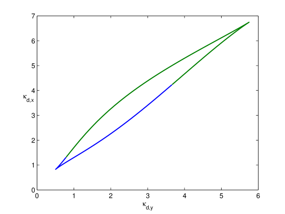
Figure 5: The parametric plot of $\kappa_{d,x}$ versus $\kappa_{d,y}$ obtained from Equation 17 where we used the following parameters: $n_{x}=2$, $n_{y}=3$, $\Delta_{x}=12$, $\Delta_{y}=10$. The blue line is for $y(x)=y_{-}$ and the green for $y(x)=y_{+}$.

In Figure 5 we have plotted $\kappa_{d,x}(x)$ versus $\kappa_{d,y}(x)$ with $x$ as the parametric variable. Inside the region bounded by the blue line (below) and green line (above) we are assured of the existence of bistable behaviour while outside this region there will be only a single globally stable steady state. Thus, for example, for a constant value of $\kappa_{d,y}$ such that bistability is possible, then increasing $\kappa_{d,x}$ from $0$ there will be a minimal value $\kappa_{d,x-}$ at which bistability is first seen and this will persist as $\kappa_{d,x}$ is increased until a second value $\kappa_{d,x-}<\kappa_{d,x+}$ is reached where the bistable behaviour once again disappears. In Figure 6 we have shown how the change of the parameter $\Delta_{y}$ influences the shape and position of the region of parameters $\kappa_{d,y}$ and $\kappa_{d,x}$ where a bistable behaviour is possible. It is clear that an increase in $\Delta_{y}$ corresponds to a decrease in the leakage, and our results show a clear expansion in the size of the region of bistability as well as a shift in $(\kappa_{d,y},\kappa_{d,x})$ space. This is the same observation made in Mackey et al (2011).

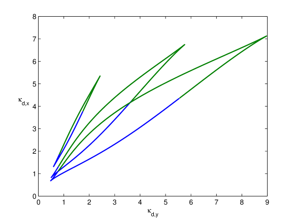
Figure 6: As in Figure 5 but with varying parameter $\Delta_{y}\in\{5,10,15\}$, from left to right.

3.3 Local and global stability.

Whether or not a steady state $W^{*}$ is locally stable is completely determined by the eigenvalues that solve the equation

$$\prod_{i=1}^{2}(\lambda+\gamma_{x_{i}})(\lambda+\gamma_{y_{i}})-\prod_{i=1}^{2}\gamma_{x_{i}}\gamma_{y_{i}}\kappa_{d,x}\kappa_{d,y}f^{\prime}_{x*}f^{\prime}_{y*}=0,$$ (18)

where $f^{\prime}_{x*}=f_{x}^{\prime}(x^{*}),f^{\prime}_{y*}=f_{y}^{\prime}(y^{*})$. Equation 18 can be rewritten in the form

$$\sum_{i=1}^{4}a_{i}\lambda^{i}+a_{0}=0$$ (19)

where the $a_{i}$, $i>0$ are positive and $a_{0}=(1-\kappa_{d,x}\kappa_{d,y}f^{\prime}_{x*}f^{\prime}_{y*})\prod_{i=1}^{2}\gamma_{x_{i}}\gamma_{y_{i}}.$ By Descartes’s rule of signs, (19) has no positive roots for $f^{\prime}_{x*}f^{\prime}_{y*}\in[0,(\kappa_{d,x}\kappa_{d,y})^{-1})$ or one positive root otherwise. Denote a locally stable steady state by S, a half or neutrally stable steady state by HS, and unstable steady state by US. Then we know that there will be:

• A single steady state $W_{1}^{*}$ (S), for $\kappa_{d,x}\in[0,\kappa_{d,x-})$

• Two steady states $W_{1}^{*}$ (S) and $W_{2}^{*}=W_{3}^{*}$ (HS) for $\kappa_{d,x}=\kappa_{d,x-}$

• Three steady states $W_{1}^{*}$ (S), $W_{2}^{*}$ (US), $W_{3}^{*}$ (S) for $\kappa_{d,x}\in(\kappa_{d,x-},\kappa_{d,x+})$

• Two steady states $W_{1}^{*}=W_{2}^{*}$ (HS) and $W_{3}^{*}$ (S) for $\kappa_{d,x}=\kappa_{d,x+}$

• One steady state $W_{3}^{*}$ (S) for $\kappa_{d,x+}<\kappa_{d,x}$.

Global stability results of others complement this classification.

Theorem 1

(Othmer, 1976; Smith, 1995, Proposition 2.1, Chapter 4) For the bistable switch given by Equations 5-9, define $I_{x}=[\kappa_{d,x}\Delta_{x}^{-1},1]$ and $I_{y}=[\kappa_{d,y}\Delta_{y}^{-1},1]$. There is an attracting box $B\subset\mathbb{R}_{4}^{+}$, where

$$B=\{(x_{i},y_{i}):x_{1,2}\in I_{x},y_{1,2}\in I_{y}\},$$

for which the flow $S_{t}$ is directed inward on the surface of $B$. All $W^{*}\in B$ and

1. If there is a single steady state, then it is globally stable.

2. If there are two locally stable steady states, then all flows $S_{t}(W^{0})$ are attracted to one of them.

4 Fast and slow variables

Identification of fast and slow variables in systems can often be used to achieve simplifications that allow quantitative examination of the relevant dynamics, and particularly to examine the approach to a steady state and the nature of that steady state. A fast variable is one that relaxes much more rapidly to an equilibrium than does a slow variable (Haken, 1983). In chemical systems this separation is often a consequence of differences in degradation rates, and the fastest variable is the one with the largest degradation rate. In recent years, with the advent of synthetic biology, investigators have engineered a variety of gene regulatory circuits, including bistable switches of the type considered here, see Hasty et al (2001); Huang et al (2012), in which they were able to experimentally control the speed with which particular variables approached a quasi-equilibrium state. Thus this experimental technique offers an experimental way to actually achieve the simplification of causing particular variables to become fast variables. We will use this technique analytically in examining the effects of noise, which has the added advantage of allowing us to derive analytic insights from the simplified model that seem to be impossible in the full model.

If it is the case that there is a single dominant slow variable in the system (5)-(8) relative to all of the other three (and here we assume without loss of generality that it is in the $X$ gene) then the four variable system describing the full switch reduces to a single equation

$$\dfrac{dx}{dt}=\gamma[\kappa_{d,x}{\mathcal{F}}(x)-x],$$ (20)

and $\gamma$ is the dominant (smallest) degradation rate. (Here, and subsequently, to simplify the notation we will drop the subscript $x$ whenever there will not be any confusion when treating the situation with a single dominant slow variable.)

5 Transcriptional and translational bursting

It has been quite clearly shown (Cai et al, 2006; Chubb et al, 2006; Golding et al, 2005; Raj et al, 2006; Sigal et al, 2006; Yu et al, 2006) that in a number of experimental situations some organisms transcribe mRNA discontinuously and as a consequence there is a discontinuous production of the corresponding effector proteins (i.e. protein is produced in bursts). Experimentally, the amplitude of protein production through bursting translation of mRNA is exponentially distributed at the single cell level with density

$$h(y)=\dfrac{1}{\bar{b}}e^{-y/{\bar{b}}},$$ (21)

where $\bar{b}$ is the average burst size, and the frequency of bursting $\varphi$ is dependent on the level of the effector. Writing Equation 21 in terms of our dimensionless variables we have

$$h(x)=\dfrac{1}{b}e^{-x/{b}}.$$ (22)

When bursting is present, the analog of the deterministic single slow variable dynamics discussed above is

$$\dfrac{dx}{dt}=-\gamma x+\Xi(h,\varphi(x)),\quad\mbox{with}\quad\varphi(x)=\gamma\varphi_{m}\mathcal{F}(x),$$ (23)

where $\Xi(h,\varphi)$ denotes a jump Markov process, occurring at a rate $\varphi$, whose amplitude is distributed with density $h$ as given in (22). Set $\kappa_{b}=\varphi_{m}$, so $\mathcal{F}$ has the same form as (12) but with $\kappa_{d,y}$ replaced by $\kappa_{b,y}$. When we have bursting dynamics described by the stochastic differential equation (23), it has been shown (Mackey and Tyran-Kamińska, 2008) that the evolution of the density $u(t,x)$ is governed by the integro-differential equation

$$\begin{split}\dfrac{\partial u(t,x)}{\partial t}-\gamma\dfrac{\partial(xu(t,x))}{\partial x}&=-\gamma\kappa_{b,x}\mathcal{F}(x)u(t,x)\\ &\quad+\gamma\kappa_{b,x}\int_{0}^{x}\mathcal{F}(z)u(t,z)h(x-z)dz.\end{split}$$ (24)

In a steady state the (stationary) solution $u_{*}(x)$ of (24) is found by solving

$$-\dfrac{d(xu_{*}(x))}{dx}=-\kappa_{b,x}\mathcal{F}(x)u_{*}(x)+\kappa_{b,x}\int_{0}^{x}\mathcal{F}(z)u_{*}(z)h_{x}(x-z)dz.$$

If $u_{*}(x)$ is unique, then the solution $u(t,x)$ of Equation 24 is said to be asymptotically stable (Lasota and Mackey, 1994) in that

$$\lim_{t\to\infty}\int_{0}^{\infty}|u(t,x)-u_{*}(x)|dx=0$$

for all initial densities $u(0,x)$. Somewhat surprisingly, it is possible to actually obtain a closed form solution for $u_{*}(x)$ as given in the following

Theorem 2

(Mackey and Tyran-Kamińska, 2008, Theorem 7). The unique stationary density of Equation 24, with $\mathcal{F}$ given by Equation 12 and $h$ given by (22), is

$$u_{*}(x)=\dfrac{\mathcal{C}}{x}e^{-x/b}\exp\left[\kappa_{b,x}\int^{x}\frac{\mathcal{F}(z)}{z}dz\right],$$ (25)

$\mathcal{C}$ is a normalization constant such that $\int_{0}^{\infty}u_{*}(x)dx=1$, and $u(t,x)$ is asymptotically stable.

Note that $u_{*}$ can be written as

$$u_{*}(x)=\mathcal{C}\exp\int^{x}\left(\dfrac{\kappa_{b,x}\mathcal{F}(z)}{z}-\frac{1}{b}-\frac{1}{z}\right)dz.$$ (26)

Thus from (26) we can write

$$u_{*}^{\prime}(x)=u_{*}(x)\left(\dfrac{\kappa_{b,x}\mathcal{F}(x)}{x}-\frac{1}{b}-\frac{1}{x}\right),$$ (27)

so for $x>0$ we have $u_{*}^{\prime}(x)=0$ if and only if

$$\dfrac{1}{\kappa_{b,x}}\left(\dfrac{x}{b}+1\right)=\mathcal{F}(x).$$ (28)

An easy graphical argument shows there may be zero to three positive roots of Equation 28, and if there are three roots we denote them by $\bar{x}_{1}<\bar{x}_{2}<\bar{x}_{3}$. The graphical arguments in conjunction with (27) show that two general cases must be distinguished, exactly as was found in Mackey et al (2011). (In what follows, $\kappa_{b,x}$, $\kappa_{b,x-}$, and $\kappa_{b,x+}$ play exactly the same role as do $\kappa_{d,x}$, $\kappa_{d,x-}$, and $\kappa_{d,x+}$ in the discussion around Figure 5.)

Case 1. $0<\kappa_{b,x}<\mathcal{F}_{0}^{-1}$. In this case, $u_{*}(0)=\infty$. If $\kappa_{b,x}<\kappa_{b,x-}$, there are no positive solutions, and $u_{*}$ will be a monotone decreasing function of $x$. If $\kappa_{b,x}>\kappa_{b,x-}$, there are two positive solutions ($\tilde{x}_{2}$ and $\tilde{x}_{3}$), and a maximum in $u_{*}$ at $\tilde{x}_{3}$ with a minimum in $u_{*}$ at $\tilde{x}_{2}$.

Case 2. $0<\mathcal{F}_{0}^{-1}<\kappa_{b,x}$. Now, $u_{*}(0)=0$ and either there are one, two, or three positive roots of Equation 28. When there are three, $\tilde{x}_{1},\tilde{x}_{3}$ will correspond to the location of maxima in $u_{*}$ and $\tilde{x}_{2}$ will be the location of the minimum between them. The condition for the existence of three roots is $\kappa_{b,x-}<\kappa_{b,x}<\kappa_{b,x+}$.

Thus we can classify the stationary density $u_{*}$ for a bistable switch as:

1. Unimodal type 1: $u_{*}(0)=\infty$ and $u_{*}$ is monotone decreasing for $0<\kappa_{b,x}<\kappa_{b,x-}$ and $0<\kappa_{b,x}<\mathcal{F}_{0}^{-1}$

2. Unimodal type 2: $u_{*}(0)=0$ and $u_{*}$ has a single maximum at

   1. $\tilde{x}_{1}>0$ for $\mathcal{F}_{0}^{-1}<\kappa_{b,x}<\kappa_{b,x-}$ or

   2. $\tilde{x}_{3}>0$ for $\kappa_{b,x+}<\kappa_{b,x}$ and $\mathcal{F}_{0}^{-1}<\kappa_{b,x}$

3. Bimodal type 1: $u_{*}(0)=\infty$ and $u_{*}$ has a single maximum at $\tilde{x}_{3}>0$ for $\kappa_{b,x-}<\kappa_{b,x}<\mathcal{F}_{0}^{-1}$

4. Bimodal type 2: $u_{*}(0)=0$ and $u_{*}$ has two maxima at $\tilde{x}_{1},\tilde{x}_{3}$, $0<\tilde{x}_{1}<\tilde{x}_{3}$ for $\kappa_{b,x-}<\kappa_{b,x}<\kappa_{b,x+}$ and $\mathcal{F}_{0}^{-1}<\kappa_{b,x}$

Note in particular from (28) that a decrease in the leakage (equivalent to an increase in $\mathcal{F}_{0}^{-1}$) facilitates a transition between unimodal and bimodal stationary distributions and that this is counterbalanced by a increases in the bursting parameters $\kappa_{b}$ and $b$. Precisely the same conclusion was obtained by Huang et al (2015) and Ochab-Marcinek and Tabaka (2015) on analytic and numerical grounds.

The exact determination of these three roots is difficult in general because of the complexity of $\mathcal{F}$, but we can derive implicit criteria for when there are exactly two roots ($\bar{x}_{1}$ and $\bar{x}_{3}$) by determining when the graph of the left hand side of (28) is tangent to $\mathcal{F}$. Using this tangency condition, differentiation of (28) yields

$$\dfrac{1}{\kappa_{b,x}b}=\mathcal{F}^{\prime}(x).$$ (29)

Although Equations 28 and 29 offer conceptually simple conditions for delineating when there are exactly two roots (and thus to find boundaries between monostable and bistable stationary densities $u_{*}$), a moments reflection after looking at (12) for $\mathcal{F}$ reveals that it is algebraically quite difficult to obtain quantitative conditions in general. However, (28) and (29) are easily used in determining numerically boundaries between monostable and bistable stationary densities.

5.1 Monomeric repression of one of the genes with bursting $(n_{x}=1)$

Evaluation of the integral appearing in Equation 25 can be carried out for all (positive) integer values of $(n_{x},n_{y})$ in theory, but the calculations become algebraically complicated. However, if we consider the situation when a single molecule of the protein from the $y$ gene is capable of repressing the $x$ gene, so $n_{x}=1$, then the results become more tractable and allow us to examine the role of different parameters in determining the nature of $u_{*}$.

Thus, for $n_{x}=1$, $\mathcal{F}$ takes the simpler form

$$\mathcal{F}(x)=\dfrac{(1+\kappa_{b,y})+(\Delta_{y}+\kappa_{b,y})x^{n_{y}}}{\Lambda+\Gamma x^{n_{y}}},$$

where

$$\Lambda=1+\Delta_{x}\kappa_{b,y}>0,\quad\Gamma=\Delta_{y}+\Delta_{x}\kappa_{b,y}>0.$$

Evaluating (25) we have the explicit representation

$$u_{*}(x)={\mathcal{C}}e^{-x/b}x^{A-1}[\Lambda+\Gamma x^{n_{y}}]^{\theta}$$ (30)

with

$$A=\dfrac{\kappa_{b,x}(1+\kappa_{b,y})}{\Lambda}>0,\quad\theta=\dfrac{\kappa_{b,x}\kappa_{b,y}(\Delta_{x}-1)(\Delta_{y}-1))}{n_{y}\Lambda\Gamma}>0.$$

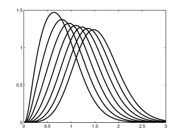
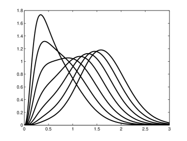
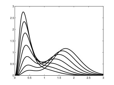
Figure 7: In this figure we illustrate stationary densities given by Equation 30 where the parameter values in each panel are taken to be $\kappa_{b,y}=1$, $\Delta_{x}=12$, $\Delta_{y}=10$, $\kappa_{b,x}\in[25,37]$ changes by 2, where the graph with highest maximum corresponds to $\kappa_{b,x}=25$ and the maxima are decreasing when $\kappa_{b,x}$ is increased. The parameter $n_{y}$ is taken in an increasing order to be $2,3,4,6$, so that we start with $n_{y}=2$ in panel (A) and have $n_{y}=6$ in panel (D).

In Figure 7 we have illustrated the form of $u_{*}(x)$ in four different situations. Figures 7 A,B show a smooth variation in a Unimodal Type 2 density as $\kappa_{b,x}\in[25,37]$ is varied by steps of 2 for $n_{y}=2$ and $n_{y}=3$ respectively. The behavior is quite different in Figures 7 C,D however for there, with $n_{y}=4$ and $n_{y}=6$, the form of $u_{*}(x)$ varies from a Unimodal Type 2 to a Bimodal Type 2 and back again as $\kappa_{b,x}$ is varied.

5.2 ‘Bang-bang’ repression with bursting

We can partially circumvent the algebraic difficulties of the previous sections by considering a limiting case. Consider the situation in which $n_{y}$ becomes large so $f_{y}(x)$ approaches the simpler form

$$f_{y}(x)\to\left\{\begin{array}[]{ll}1,&0\leq x<\theta,\\ \Delta_{y}^{-1},&\theta\leq x,\end{array}\right.$$

where

$$\theta\simeq\dfrac{1}{\sqrt[n_{y}]{\Delta_{y}}}\sqrt[n_{y}]{\dfrac{n_{y}-1}{n_{y}+1}}\to\dfrac{1}{\sqrt[n_{y}]{\Delta_{y}}}\to 1,$$

so we have

$$\mathcal{F}(x)\to\left\{\begin{array}[]{ll}\mathcal{F}_{0}=\dfrac{1+\kappa_{b,y}^{n_{y}}}{1+\Delta_{x}\kappa_{b,y}^{n_{x}}},&0\leq x<1,\\ \mathcal{F}_{\infty}=\dfrac{1+(\kappa_{b,y}/\Delta_{y})^{n_{y}}}{1+\Delta_{x}(\kappa_{b,y}/\Delta_{y})^{n_{x}}},&1\leq x.\end{array}\right.$$ (31)

The evaluation of (25) is simple and yields a stationary density which is (piecewise) that of the gamma distribution:

$$u_{*}(x)=\mathcal{C}e^{-x/b}x^{A(x)-1}$$

where

$$A(x)=\left\{\begin{array}[]{ll}A_{0}\equiv{\kappa_{b,x}\mathcal{F}_{0}},&0\leq x<1,\\ A_{\infty}\equiv{\kappa_{b,x}\mathcal{F}_{\infty}},&1\leq x.\end{array}\right.$$

Note that $u_{*}(x)$ is continuous but not differentiable at $x=1$, and $\mathcal{C}$ is given explicitly by

$$\mathcal{C}=\dfrac{1}{b^{A_{0}}[\Gamma(A_{0})-\Gamma(A_{0},1/b)]+b^{A_{\infty}}\Gamma(A_{\infty})},$$

where $\Gamma(\alpha)$ is the gamma function and $\Gamma(\alpha,\beta)$ is the incomplete gamma function.

In this limiting case the stationary density may display one of three general forms as we have classified the densities earlier. Namely:

1. If $\kappa_{b,x}<\mathcal{F}_{0}^{-1}$ and $\kappa_{b,x}<\mathcal{F}_{\infty}^{-1}$ then $u_{*}(x)$ will be of Unimodal type 1;

2. If $\kappa_{b,x}<\mathcal{F}_{0}^{-1}$ and $\kappa_{b,x}>\mathcal{F}_{\infty}^{-1}$ then $u_{*}(x)$ will be Bimodal type 1;

3. If $\kappa_{b,x}>\mathcal{F}_{0}^{-1}$ (which implies $\kappa_{b,x}>\mathcal{F}_{\infty}^{-1}$) then $u_{*}(x)$ will be Bimodal type 2.

6 Gaussian distributed noise in the molecular degradation rate

For a generic one dimensional stochastic differential equation of the form

$$dx(t)=\alpha(x)dt+\sigma(x)dw(t),$$

where $w$ is a standard Brownian motion, the corresponding Fokker Planck equation

$$\dfrac{\partial u}{\partial t}=-\dfrac{\partial(\alpha u)}{\partial x}+\dfrac{1}{2}\dfrac{\partial^{2}(\sigma^{2}u)}{\partial x^{2}}$$ (32)

can be written in the form of a conservation equation

$$\dfrac{\partial u}{\partial t}+\dfrac{\partial J}{\partial x}=0,$$

where

$$J=\alpha u-\frac{1}{2}\dfrac{\partial(\sigma^{2}u)}{\partial x}$$

is the probability current. In a steady state when $\partial_{t}u\equiv 0$, the current must satisfy $J=\mbox{constant}$ throughout the domain of the problem. In the particular case when $J=0$ at one of the boundaries (a reflecting boundary) then $J=0$ for all $x$ in the domain and the steady state solution $u_{*}$ of Equation 32 is easily obtained with a single quadrature as

$$u_{*}(x)=\dfrac{\mathcal{C}}{\sigma^{2}(x)}\exp\left\{2\int^{x}\dfrac{\alpha(y)}{\sigma^{2}(y)}dy\right\},$$

where $\mathcal{C}$ is a normalizing constant as before.

In our considerations of the effects of continuous fluctuations, we examine the situation in which Gaussian fluctuations appear in the degradation rate $\gamma_{x}$ of the generic equation (20). Gillespie (2000) has shown that in this situation we need to consider what he calls the chemical Langevin equation, so (20) takes the form

$$dx=\gamma[\kappa_{d,x}\mathcal{F}(x)-x]dt+\sqrt{\gamma x}dw.$$

(In the situation we consider here, $\alpha(x)=\gamma[\kappa_{d,x}\mathcal{F}(x)-x]$ and $\sigma(x)=\sigma_{\gamma}\sqrt{x}$.) Within the Ito interpretation of stochastic integration, this equation has a corresponding Fokker Planck equation for the evolution of the ensemble density $u(t,x)$ given by

$$\dfrac{\partial u}{\partial t}=-\dfrac{\partial\left[\gamma(\kappa_{d,x}\mathcal{F}(x)-x)u\right]}{\partial x}+\dfrac{{\gamma}}{2}\dfrac{\partial^{2}(xu)}{\partial x^{2}}.$$ (33)

Since concentrations of molecules cannot become negative the boundary at $x=0$ is reflecting and the stationary solution of Equation 33 is given by

$$u_{*}(x)=\dfrac{\mathcal{C}}{x}e^{-2x}\exp\left[2\kappa_{d,x}\int^{x}\frac{\mathcal{F}(z)}{z}dz\right].$$ (34)

We have also the following result.

Theorem 3

(Pichór and Rudnicki, 2000, Theorem 2). The unique stationary density of Equation 33 is given by Equation 34. Further $u(t,x)$ is asymptotically stable.

Remark 1

Note that the stationary solution for the density $u_{*}(x)$ given by Equation 34 in the presence of noise in the protein degradation rate is identical to the solution in Equation 25, when transcriptional and/or translational noise in present in the system, as long as we make the identification of $\kappa_{b,x}$ with $2\kappa_{d,x}$ and $b$ with $1/2$. As a consequence, all of the results of the analysis in Section 5 are applicable in this section. The implication is, of course, that one cannot distinguish between the location of the noise simply based on the nature of the stationary density.

7 Two dominant slow genes with bursting

In this last section we turn our attention to the situation in which we have two slow variables, one in each gene. If there are two slow variables with one in each of the $X$ and $Y$ genes, then we obtain a two dimensional system that is significantly different and more difficult to deal with from what we have encountered so far, and we wish to examine the existence of the stationary density $u_{*}(x,y)$ in the presence of bursting production.

For two dominant slow variables in different genes with bursting, the stochastic analogs of the deterministic equations are

$$\dfrac{dx}{dt} =-\gamma_{x}x+\Xi(h_{1},\varphi_{1}(y))\quad\mbox{with}\quad\varphi_{1}(y)=\gamma_{x}\kappa_{b,x}f_{x}(y),$$

$$\dfrac{dy}{dt} =-\gamma_{y}y+\Xi(h_{2},\varphi_{2}(x))\quad\mbox{with}\quad\varphi_{2}(x)=\gamma_{y}\kappa_{b,y}f_{y}(x).$$

To be more specific, let $x(t)$ and $y(t)$ denote the amount of protein in a cell at time $t$, $t\geq 0$, produced by gene $X$ and $Y$, respectively. If only degradation were present, then $(x(t),y(t))$ would satisfy the equation

$$x^{\prime}(t)=-\gamma_{x}x(t),\quad y^{\prime}(t)=-\gamma_{y}y(t),\quad t\geq 0.$$ (35)

The solution of (35) starting at time $t_{0}=0$ from $(x_{0},y_{0})\in\mathbb{R}_{+}^{2}$ is of the form

$$\pi_{t}(x_{0},y_{0})=(e^{-\gamma_{x}t}x_{0},e^{-\gamma_{y}t}y_{0}),\quad t\geq 0.$$

But, we interrupt the degradation at random times

$$0=t_{0}<t_{1}<t_{2}<\ldots$$

when, independently of everything else, a random amount of protein $x$ or $y$ is produced according to an exponential distribution with mean $b_{x}$ or $b_{y}$, respectively, with densities

$$h_{1}(x)=\dfrac{1}{b_{x}}e^{-x/{b_{x}}},\quad h_{2}(y)=\dfrac{1}{b_{y}}e^{-y/{b_{y}}}.$$

The rate of production of protein $x$ (protein $y$) depends on the level of protein $y$ (protein $x$) and is $\varphi_{1}(y)$ ($\varphi_{2}(x)$). Consequently, at each $t_{k}$ if $x(t_{k})=x$ and $y(t_{k})=y$ then one of the genes $X$ or $Y$ can be chosen at random with probabilities $p_{1}$ or $p_{2}$, respectively, given by

$$p_{1}(x,y)=\frac{\varphi_{1}(y)}{\varphi(x,y)},\quad p_{2}(x,y)=\frac{\varphi_{2}(x)}{\varphi(x,y)},$$

and we have

$$\Pr(t_{k+1}-t_{k}>t|x(t_{k})=x,y(t_{k})=y)=e^{-\int_{0}^{t}\varphi(\pi_{s}(x,y))ds},\quad t>0,$$

where the function $\varphi$ is of the form

$$\varphi(x,y)=\varphi_{1}(y)+\varphi_{2}(x)=\gamma_{x}\kappa_{b,x}f_{x}(y)+\gamma_{y}\kappa_{b,y}f_{y}(x).$$

The process $Z(t)=(x(t),y(t))$ is a Markov process with values in $E=[0,\infty)^{2}=\mathbb{R}_{+}^{2}$ given by

$$Z(t)=\left\{\begin{array}[]{ll}\pi_{t-t_{k-1}}(Z(t_{k-1})),&t_{k-1}\leq t<t_{k},\\ Z(t_{k}-)+\xi_{k},&t=t_{k},k=1,2,\ldots\end{array}\right.$$

where

$$Z(t_{k}-)=\pi_{t_{k}-t_{k-1}}(Z(t_{k-1}))$$

and $(\xi_{k})_{k\geq 1}$ is a sequence of random variables such that

$$\Pr(Z(t_{k}-)+\xi_{k}\in B|Z(t_{k}-)=z)=\mathcal{P}(z,B)$$

with

$$\mathcal{P}(z,B)=p_{1}(z)\int_{0}^{\infty}1_{B}(z+\theta e_{1})h_{1}(\theta)d\theta\\ +p_{2}(z)\int_{0}^{\infty}1_{B}(z+\theta e_{2})h_{2}(\theta)d\theta.$$

Here $e_{1}$ and $e_{2}$ are the unit vectors from $\mathbb{R}^{2}$

$$e_{1}=\left(\begin{array}[]{c}1\\ 0\\ \end{array}\right),\quad e_{2}=\left(\begin{array}[]{c}0\\ 1\\ \end{array}\right).$$

Let $\mathbb{P}_{z}$ be the distribution of the process $Z=\{Z(t)\}_{t\geq 0}$ starting at $Z(0)=z$ and $\mathbb{E}_{z}$ the corresponding expectation operator. For any $z$ and any Borel subset of $\mathbb{R}^{2}_{+}$ we have

$$\mathbb{P}_{z}(Z(t)\in B)=\sum_{n=0}^{\infty}\mathbb{P}_{z}(Z(t)\in B,t_{n}\leq t<t_{n+1}).$$

If the distribution of $Z(0)$ has a probability density $u_{0}$ with respect to the Lebesgue measure $m$ on $\mathbb{R}_{+}^{2}$ then $Z(t)$ has the distribution with density $P(t)u_{0}$, i.e.,

$$\int_{E}\mathbb{P}_{z}(Z(t)\in B)u_{0}(z)m(dz)=\int_{B}P(t)u_{0}(z)m(dz),\quad B\in\mathcal{B}(\mathbb{R}_{+}^{2}).$$ (36)

The evolution equation for the density $u(t,x,y)=P(t)u_{0}(x,y)$ is

$$\begin{split}\dfrac{\partial u}{\partial t}-\gamma_{x}\dfrac{\partial(xu)}{\partial x}-\gamma_{y}\dfrac{\partial(yu)}{\partial y}&=-\varphi(x,y)u(t,x,y)\\ &\quad+\varphi_{1}(y)\int_{0}^{x}h_{1}(x-z_{x})u(t,z_{x},y)dz_{x}\\ &\quad+\varphi_{2}(x)\int_{0}^{y}h_{2}(y-z_{y})u(t,x,z_{y})dz_{y},\end{split}$$ (37)

with initial condition $u(0,x,y)=u_{0}(x,y)$, $x,y\in[0,\infty)$.

Theorem 4

There is a unique density $u_{*}(x,y)$ which is a stationary solution of (37) and $u(t,x,y)$ is asymptotically stable.

Proof

We use the notation of Rudnicki et al (2002) and apply (Rudnicki et al, 2002, Theorem 5) together with (Pichór and Rudnicki, 2000, Theorem 1). Let $E=\mathbb{R}^{2}_{+}$ and $m$ be the Lebesgue measure on $E$. The evolution equation (37) induces a strongly continuous semigroup $\{P(t)\}_{t\geq 0}$ of Markov operators on the space of Lebesgue integrable functions $L^{1}=L^{1}(E,\mathcal{B}(E),m)$ (see e.g. Tyran-Kamińska (2009)). Recall that a function $f\colon E\to\mathbb{R}_{+}$ is called lower semicontinuous, if

$$\liminf_{w\to z}f(w)\geq f(z)$$

for every $z\in E$. We show that there exists a nonnegative Borel function $q$ defined on $(0,\infty)\times E\times E$ with the following properties

1. for each $t>0$ and each Borel set $B$

   $$\mathbb{P}_{z}(Z(t)\in B)\geq\int_{B}q(t,w,z)m(dw)\quad\text{for all }z\in E,$$

2. for each $t>0$ the function $(w,z)\mapsto q(t,w,z)$ is lower semicontinuous,

3. for each $z$ there exists $t>0$ such that

   $$\int_{E}q(t,w,z)m(dw)>0,$$

4. for $m$-a.e. $z\in E$ and every Borel set $B$ with $m(B)>0$

   $$\int_{0}^{\infty}\int_{B}q(t,w,z)m(dw)dt>0.$$

Then it follows from (Rudnicki et al, 2002, Theorem 5) and (Pichór and Rudnicki, 2000, Theorem 1) that either $u(t,x,y)$ is asymptotically stable or the process $Z$ is sweeping from compact subsets of $E$, i.e.,

$$\lim_{t\to\infty}\int_{E}\mathbb{P}_{z}(Z(t)\in F)u_{0}(z)m(dz)=0$$ (38)

for all compact sets $F\subset E$ and all densities $u_{0}$. We have

$$\begin{split}\mathbb{P}_{z}(Z(t)\in B)=\sum_{n=0}^{\infty}\mathbb{P}_{z}(\pi_{t-t_{n}}Z(t_{n})\in B,t_{n}\leq t<t_{n+1}).\end{split}$$

The discrete time process $(Z(t_{n}),t_{n})_{n\geq 0}$ is Markov with transition probability $P((z,s),B\times I)=Q_{z}(B\times((I-s)\cap\mathbb{R}_{+}))$ for Borel subsets $B$ of $\mathbb{R}^{2}_{+}$ and Borel subsets $I$ of $\mathbb{R}_{+}$, where $Q$ is given by

$$Q_{z}(B\times I)=\mathbb{P}_{z}(Z(t_{1})\in B,t_{1}\in I)=\\ \sum_{i=1}^{2}\int_{I}\int_{0}^{\infty}1_{B}(\pi_{s_{1}}z+\theta e_{i})\varphi(\pi_{s_{1}}z)e^{-\phi_{z}(s_{1})}p_{i}(\pi_{s_{1}}z)h_{i}(\theta)d\theta ds_{1}.$$

We have

$$\mathbb{P}_{z}(\pi_{t-t_{1}}(Z(t_{1}))\in B,t_{1}\leq t<t_{2})=\int_{E\times[0,t]}1_{B}(\pi_{t-s_{1}}z_{1})e^{-\phi_{z_{1}}(t-s_{1})}Q_{z}(dz_{1},ds_{1})$$

and for $k=2$ we obtain

$$\mathbb{P}_{z}(\pi_{t-t_{2}}(Z(t_{2}))\in B,t_{2}\leq t<t_{3})=\\ \int_{E\times[0,t]}\int_{E\times[0,t-s_{1}]}1_{B}(\pi_{t-(s_{2}+s_{1})}z_{2})e^{-\phi_{z_{2}}(t-(s_{2}+s_{1}))}Q_{z_{1}}(dz_{2},ds_{2})Q_{z}(dz_{1},ds_{1}).$$

Since $\varphi$ is bounded from above by a constant $\overline{\varphi}$ and $\varphi p_{i}=\varphi_{i}$ is bounded from below by a constant $c_{i}>0$, we obtain that

$$Q_{z}(B\times I)\geq\int_{I}\int_{0}^{\infty}\sum_{i=1}^{2}1_{B}(\pi_{s_{1}}z+\theta e_{i})e^{-\overline{\varphi}s_{1}}c_{i}h_{i}(\theta)d\theta ds_{1}$$

for all $z$. Now, if $z_{1}=\pi_{s_{1}}z+\theta_{1}e_{1}$ and $z_{2}=\pi_{s_{2}}z_{1}+\theta_{2}e_{2}$, then

$$\begin{split}\pi_{t-(s_{2}+s_{1})}z_{2}&=\pi_{t}z+\pi_{t-s_{1}}(\theta_{1}e_{1})+\pi_{t-(s_{2}+s_{1})}(\theta_{2}e_{2})\\ &=\pi_{t}z+T_{(s_{1},s_{2})}(\theta_{1},\theta_{2}),\end{split}$$

where

$$T_{(s_{1},s_{2})}(\theta_{1},\theta_{2})=(\theta_{1}e^{-\gamma_{1}(t-s_{1})},\theta_{2}e^{-\gamma_{2}(t-(s_{2}+s_{1}))}).$$

Consequently, we obtain

$$\mathbb{P}_{z}(Z(t)\in B)\geq\\ \int_{0}^{t}\int_{0}^{t-s_{1}}\int_{0}^{\infty}\int_{0}^{\infty}1_{B}(\pi_{t}z+T_{(s_{1},s_{2})}(\theta_{1},\theta_{2}))e^{-\overline{\varphi}t}c_{1}c_{2}h_{1}(\theta_{1})h_{2}(\theta_{2})d\theta_{2}d\theta_{1}ds_{2}ds_{1}.$$

The transformation $(\theta_{1},\theta_{2})\mapsto T_{(s_{1},s_{2})}(\theta_{1},\theta_{2})$ is invertible on $(0,\infty)^{2}$, thus we can make a change of variables under the integral to conclude that

$$\mathbb{P}_{z}(Z(t)\in B)\geq\int_{(0,\infty)^{2}}1_{B}(\pi_{t}z+w)e^{-(\overline{\varphi}+\gamma_{1}+\gamma_{2})t}\widetilde{q}(t,w)dw,$$

where

$$\widetilde{q}(t,(w_{1},w_{2}))=\\ \int_{0}^{t}\int_{0}^{t-s_{1}}e^{\gamma_{1}s_{1}+\gamma_{2}(s_{1}+s_{2})}c_{1}c_{2}h_{1}(e^{\gamma_{1}(t-s_{1})}w_{1})h_{2}(e^{\gamma_{2}(t-s_{1}-s_{2})}w_{2})ds_{2}ds_{1}.$$

Consequently, we obtain

$$\mathbb{P}_{z}(Z(t)\in B)\geq\int_{B}q(t,w,z)dw,$$

where

$$q(t,w,z)=e^{-(\overline{\varphi}+\gamma_{1}+\gamma_{2})t}\widetilde{q}(t,w-\pi_{t}z)1_{(0,\infty)^{2}}(w-\pi_{t}z),\quad w,z\in E.$$

For each $t>0$ the function $(w,z)\mapsto q(t,w,z)$ is lower semicontinuous and

$$\int_{E}q(t,w,z)dw>0$$

for every $z$. Finally, to check the last condition note that $\pi_{t}z$ converges to zero as $t\to\infty$ for every $z$. Thus, for every $z\in E$ and $w\in(0,\infty)^{2}$ we can find $t_{0}>0$ such that $w-\pi_{t}z\in(0,\infty)^{2}$ for every $t\geq t_{0}$, which implies that

$$\int_{0}^{\infty}q(t,w,z)dt>0$$

for all $z\in E$ and $w\in(0,\infty)^{2}$.

Next, we show that the process is not sweeping from compact subsets. Suppose, contrary to our claim, that the process is sweeping. It follows from (38) that for every compact set $F$ and every density $u_{0}$ we have

$$\lim_{t\to\infty}\frac{1}{t}\int_{0}^{t}\int_{E}\mathbb{P}_{z}(Z(s)\in F)u_{0}(z)m(dz)=0.$$

Chebyshev inequality implies that

$$\mathbb{P}_{z}(Z(t)\in F_{a})\geq 1-\frac{1}{a}\mathbb{E}_{z}V(Z(t))$$

for all $t>0$, $z\in E$, and $a>0$, where $V$ is a nonnegative measurable function and $F_{a}=\{z\in E:V(z)\leq a\}$. To get a contradiction it is enough to show that

$$\limsup_{t\to\infty}\frac{1}{t}\int_{0}^{t}\int_{E}\mathbb{E}_{z}V(Z(s))u_{0}(z)m(dz)ds<\infty$$

for a density $u_{0}$ and a continuous function $V$ such that each $F_{a}$ is a compact subset of $E$. Recall that an operator $\mathcal{L}$ is the extended generator of the Markov process $Z$, if its domain $\mathcal{D}(\mathcal{L})$ consists of those measurable $V\colon E\to\mathbb{R}$ for which there exists a measurable $U\colon E\to\mathbb{R}$ such that for each $z\in E$, $t>0$,

$$\mathbb{E}_{z}(V(Z(t)))=V(z)+\mathbb{E}_{z}\left(\int_{0}^{t}U(Z(s))\,ds\right)$$

and

$$\int_{0}^{t}\mathbb{E}_{z}(|U(Z(s))|)ds<\infty,$$

in which case we define $\mathcal{L}V=U$. From (Davis, 1993, Theorem 26.14 and Remark 26.16) it follows that

$$\mathcal{L}V(z)=\mathcal{L}_{0}V(z)+\varphi(z)\int_{E}(V(w)-V(z))\mathcal{P}(z,dw),$$

where for $z=(x,y)$ we have

$$\mathcal{L}_{0}V(x,y)=-\gamma_{1}x\frac{\partial V}{\partial x}(x,y)-\gamma_{2}y\frac{\partial V}{\partial y}(x,y)$$

and that $V$ belongs to the domain of $\mathcal{L}$ if the function $t\mapsto V(\pi_{t}(x,y))$ is absolutely continuous and for each $t$

$$\mathbb{E}(\sum_{n:t_{n}\leq t}|V(Z(t_{n}))-V(Z(t_{n}-))|)<\infty.$$

Observe that for $V(x,y)=x+y$ this condition holds and we obtain

$$\mathcal{L}V(x,y)=-(\gamma_{x}+\gamma_{y})V(x,y)+\varphi(x,y)(b_{x}p_{1}(x,y)+b_{y}p_{2}(x,y)).$$

Consequently, there are positive constants $c_{1}$ and $c_{2}$ such that for all $z=(x,y)$ we have

$$\mathcal{L}V(z)\leq-c_{1}V(z)+c_{2},$$

which implies that

$$\mathbb{E}_{z}(V(Z(t)))\leq V(z)-c_{1}\int_{0}^{t}\mathbb{E}_{z}V(Z(s))\,ds+c_{2}t.$$

Hence, for each $t>0$ and $z\in E$ we have

$$\frac{1}{t}\int_{0}^{t}\mathbb{E}_{z}V(Z(s))\,ds\leq\frac{c_{2}}{c_{1}}+\frac{1}{c_{1}t}V(z).$$

Taking a density $u_{0}$ with $\int_{E}V(z)u_{0}(z)m(dz)<\infty$ completes the proof.

Remark 2

Observe that

$$\frac{\partial}{\partial x}\int_{0}^{x}h_{1}(x-z_{x})u_{*}(z_{x},y)dz_{x}=\frac{1}{b_{x}}\left(u_{*}(x,y)-\int_{0}^{x}h_{1}(x-z_{x})u_{*}(z_{x},y)dz_{x}\right).$$

Thus the equation for the stationary density $u_{*}(x,y)$ can be rewritten as

$$\frac{\partial}{\partial x}\left(\gamma_{x}xu_{*}(x,y)-\varphi_{1}(y)e^{-x/b_{x}}\int_{0}^{x}e^{z_{x}/b_{x}}u_{*}(z_{x},y)dz_{x}\right)\\ +\frac{\partial}{\partial y}\left(\gamma_{y}yu_{*}(x,y)-\varphi_{2}(x)e^{-y/b_{y}}\int_{0}^{y}e^{z_{y}/b_{y}}u_{*}(x,z_{y})dz_{y}\right)=0.$$

However, we have been unable to find an analytic solution to this equation.

8 Discussion and conclusions

Here we have considered the behavior of a bistable molecular switch in both its deterministic version as well as what happens in the presence of two different kinds of noise. The results that we have obtained in the presence of noise are, unfortunately, only partial due to the analytic difficulties in solving for the stationary density but we have been able to offer analytic expressions for $u_{*}(x)$ either in the presence of transcriptional and/or translational bursting (Section 5) or in the presence of Gaussian noise on the degradation rate (Section 6) when there is a single dominant slow variable. We have shown that in both cases one cannot distinguish between the source of the noise based on the nature of the stationary density. In the situation where there are two dominant slow variables (Section 7) we have established the asymptotic stability of $u(t,x,y)$, and thus the uniqueness of the stationary density $u_{*}(x,y)$.