Uplink Achievable Rate for Massive MIMO Systems with Low-Resolution ADC

Abstract

In this letter, we derive an approximate analytical expression for the uplink achievable rate of a massive multi-input multi-output (MIMO) antenna system when finite precision analog-digital converters (ADCs) and the common maximal-ratio combining technique are used at the receivers. To obtain this expression, we treat quantization noise as an additive quantization noise model. Considering the obtained expression, we show that low-resolution ADCs lead to a decrease in the achievable rate but the performance loss can be compensated by increasing the number of receiving antennas. In addition, we investigate the relation between the number of antennas and the ADC resolution, as well as the power-scaling law. These discussions support the feasibility of equipping highly economical ADCs with low resolution in practical massive MIMO systems.

I Introduction

Massive multi-input multi-output (MIMO) antenna technology has emerged as an attractive candidate technique for 5G mobile networks because of its potential to significantly improve the capacity of wireless communication systems [2]. Such a technique mainly uses hundreds of antennas at the base station (BS) to serve a relatively small number of user terminals on the same time-frequency channel [2, 3, 4]. Research [3] showed that simple linear processing such as maximal-ratio combining (MRC) in massive MIMO systems can achieve very high spectral efficiency. In addition, massive MIMO has been proven able to achieve a significant gain in energy efficiency [4].

The large number of antennas required in massive MIMO causes a substantial increase in hardware cost and power consumption. This fact motives studies on quantized MIMO systems [5, 6, 7], where each receiver antenna uses a very low resolution (e.g., $1-3$ bits) analog-to-digital converter (ADC). The capacity of $1$-bit quantized MIMO was studied in [5], where the exact nonlinearity property of a quantizer is considered. Rather than using the nonlinear quantizer model, studies [6, 7] treat the quantization noise as additive and independent noise, as encapsulated by the additive quantization noise model (AQNM). Although the model is an approximation, AQNM is widely used because it facilitates analysis and provides insights into quantized systems. Under AQNM, the effect of ADC resolution and bandwidth on the achievable rate were investigated in [7].

In this letter, AQNM is used in investigating the uplink achievable rate affected by quantizated massive MIMO systems. In particular, we consider an MRC receiver that can be performed in a non-centralized manner to avoid the unscalable data transport overhead required by other existing receivers (e.g., zero-forcing receiver). Under the assumption of perfect channel state information (CSI) at BS, a tight approximate expression for an achievable uplink rate that holds for arbitrary number of antennas is provided. The approximate expression agrees with previous works in [4] and [8] as the quantizers have infinite precision. On the basis of the derived expression, the relationship between the number of antennas and the ADC resolution, as well as the power-scaling law, is investigated.

II System Model

Consider the uplink of a multi-user MIMO (MU-MIMO) system formed by a BS equipped with an array of $M$ antennas and serving $N$ single antenna user terminals in the same time-frequency resource. The received $M$ dimensional vector ${\bf{y}}$ at BS can be expressed as [3]

$${\bf{y}}=\sqrt{{p_{u}}}{\bf{Gx}}+{\bf{n}},$$ (1)

where $\bf{G}$ represents the $M\times N$ channel matrix between BS and users, ${\bf{x}}$ denotes the $N\times 1$ vector of symbols transmitted by all users, ${p_{u}}$ is the average transmitted power of each user, and ${{\bf{n}}\sim{\cal C}{\cal N}\left({0,{\bf{I}}}\right)}$ is the additive white Gaussian noise vector.

We denote the independent channel coefficient between the $n$th user and the $m$th antenna at the BS as ${g_{mn}}={\left[{\bf{G}}\right]_{mn}}$, which models independent fast fading, geometric attenuation, and log-normal shadow fading [3]. The coefficient ${g_{mn}}$ can be written as

$${g_{mn}}={h_{mn}}\sqrt{{\beta_{n}}},$$ (2)

where $h_{mn}$ is the fast-fading coefficient from the $n$th user to the $m$th antenna of BS, and ${\beta_{n}}$ models both geometric attenuation and shadow fading, which is assumed to be constant across the antenna array. In matrix form, we write

$${\bf{G}}={\bf{H}}{{\bf{D}}^{{1\mathord{\left/{\vphantom{12}}\right.\kern-1.2pt}2}}},$$ (3)

where ${{\bf H}=[h_{mn}]}$ is the ${M\times N}$ fast fading matrix between the users and BS, and $\bf{D}$ is the ${N\times N}$ diagonal matrix with diagonal entries $\{\beta_{n}\}$ .

Assuming the gain of the automatic gain control is set appropriately, we use AQNM and formulate the quantizer outputs as [7]

$${{\bf{y}}_{\sf q}}=\alpha{\bf{y}}+{{\bf{n}}_{\sf q}}=\alpha\sqrt{{p_{u}}}{\bf{Gx}}+\alpha{\bf{n}}+{{\bf{n}}_{\sf q}}$$ (4)

with ${\alpha=1-\rho}$, where $\rho$ is the inverse of the signal-to-quantization-noise ratio, and ${{\bf{n}}_{\sf q}}$ is the additive Gaussian quantization noise vector that is uncorrelated with $\bf{y}$. Let $b$ be the number of quantization bins. We assume that the input to the quantizer is Gaussian. Accordingly, for the non-uniform scalar minimum mean-square-error quantizer of a Gaussian random variable, the values of $\rho$ are listed in Table I for $b\leq 5$ and can be approximated by $\rho={\textstyle{{\pi\sqrt{3}}\over 2}}\cdot{2^{{\rm{-}}2b}}$ for ${b>5}$.

TABLE I: $\rho$ for different ADC quantization bits $b$

$b$	1	2	3	4	5
$\rho$	0.3634	0.1175	0.03454	0.009497	0.002499

For a fixed channel realization $\bf{G}$, the covariance of ${{\bf{n}}_{\sf q}}$ is given by

$${{\bf{R}}_{{{\bf{n}}_{\sf q}}{{\bf{n}}_{\sf q}}}} ={\mathbb{E}}\!\left\{{{{\bf{n}}_{\sf q}}{\bf{n}}_{\sf q}^{H}\big{|}{\bf{G}}}\right\}$$

$$=\alpha\left({1-\alpha}\right){\sf diag}{\left({p_{u}{\bf{G}}{{\bf{R}}_{x}}{{\bf{G}}^{H}}+{\bf{I}}}\right)},$$ (5)

where ${{\bf{R}}_{x}}$ is the input covariance matrix . Since ${{\bf{R}}_{x}}={\bf{I}}$, (II) can be expressed as

$${{\bf{R}}_{{{\bf{n}}_{\sf q}}{{\bf{n}}_{\sf q}}}}=\alpha\left({1-\alpha}\right){\sf diag}{\left({p_{u}{\bf{G}}{{\bf{G}}^{H}}+{\bf{I}}}\right)}.$$ (6)

III Analysis of Achievable Uplink Rate

In this section, we derive a tractable approximate expression of the achievable uplink rate for the MRC receiver. Using the expression, we analyze the effect of ADC resolution on the achievable uplink rate. For the MRC receiver, the quantized signal vector is processed as

$${\bf{r}}={{\bf{G}}^{H}}{{\bf{y}}_{\sf q}}.$$ (7)

Substituting (4) into (7) results in

$${\bf{r}}=\sqrt{{p_{u}}}\alpha{{\bf{G}}^{H}}{\bf{Gx}}+\alpha{{\bf{G}}^{H}}{\bf{n}}+{{\bf{G}}^{H}}{{\bf{n}}_{\sf q}}.$$ (8)

From (8), the $n$th element of $\bf{r}$ can be expressed as

$${r_{n}}=\sqrt{{p_{u}}}\alpha{\bf{g}}_{n}^{H}{{\bf{g}}_{n}}{x_{n}}+\sqrt{{p_{u}}}\alpha\sum\limits_{i=1,i\neq n}^{N}{{\bf{g}}_{n}^{H}{{\bf{g}}_{i}}{x_{i}}}+\alpha{\bf{g}}_{n}^{H}{\bf{n}}\;+{\bf{g}}_{n}^{H}{{\bf{n}}_{\sf q}},$$ (9)

where ${{\bf{g}}_{n}}$ is the $n$th column of $\bf{G}$. Given a channel realization ${\bf{G}}$, the noise-plus-interference term is a random variable with zero mean and variance

$${\cal I}_{{\bf G}}={p_{u}}{\alpha}^{2}\sum\limits_{i=1,i\neq n}^{N}{{{\left|{{\bf{g}}_{n}^{H}{{\bf{g}}_{i}}}\right|}^{2}}}+{\alpha}^{2}{{\left\|{{{\bf{g}}_{n}}}\right\|}^{2}}\\ +\alpha\left({1-\alpha}\right){\bf{g}}_{n}^{H}{\sf diag}\left({{p_{u}}{\bf{G}}{{\bf{G}}^{H}}+{\bf{I}}}\right){{\bf{g}}_{n}}.$$ (10)

Following the assumption in [11], we model this term as additive Gaussian noise independent of ${x_{n}}$ and derive the ergodic achievable uplink rate of the $n$th user as

$${R_{n}}={\mathbb{E}}\!\left\{{{{\log}_{2}}\left({1+\frac{{{p_{u}}{\alpha^{2}}{{\left\|{{{\bf{g}}_{n}}}\right\|}^{4}}}}{{\cal I}_{{\bf G}}}}\right)}\right\},$$ (11)

where ${\cal I}_{{\bf G}}$ is given in (10), and the expectation is taken over the fast-fading coefficients $\{h_{mn}\}$. No efficient way is able to directly calculate the achievable rate in (11). Therefore, we derive an approximation that is presented as follows:

Theorem 1.

Using MRC receivers with perfect CSI in the quantized MIMO systems, we can approximate the achievable uplink rate of the $n$th user by

$${{\widetilde{R}}_{n}}={\log_{2}}{\left({1+\frac{{{p_{u}}{\alpha}{\beta_{n}}\left({M+1}\right)}}{{\cal I}}}\right)}$$ (12)

where

$${\cal I}={{p_{u}}\alpha\sum\limits_{i=1,i\neq n}^{N}{{\beta_{i}}}+{p_{u}}\left({1-\alpha}\right){\left({\sum\limits_{i=1}^{N}{{\beta_{i}}}+{\beta_{n}}}\right)}+1}.$$ (13)

Proof: Applying [8, Lemma 1], we begin by approximating $R_{n}$ with

$${{\widetilde{R}}_{n}}={\log_{2}}{\left({1+\frac{{{p_{u}}{\alpha^{2}}{\mathbb{E}}{\left\{{{{\|{{{\bf{g}}_{n}}}\|}^{4}}}\right\}}}}{{\mathbb{E}}\{{\cal I}_{{\bf G}}\}}}\right)}$$ (14)

where

$${\mathbb{E}}\{{\cal I}_{{\bf G}}\}={p_{u}}\alpha^{2}\sum\limits_{i=1,i\neq n}^{N}{{\mathbb{E}}\Big{\{}{{{\left|{{\bf{g}}_{n}^{H}{{\bf{g}}_{i}}}\right|}^{2}}}\Big{\}}}+\alpha^{2}{\mathbb{E}}\Big{\{}{{{\left\|{{{\bf{g}}_{n}}}\right\|}^{2}}}\Big{\}}\\ +\alpha\left({1-\alpha}\right){\mathbb{E}}\Big{\{}{{\bf{g}}_{n}^{H}{\sf diag}\left({{p_{u}}{\bf{G}}{{\bf{G}}^{H}}+{\bf{I}}}\right){{\bf{g}}_{n}}}\Big{\}}.$$ (15)

To obtain a tractable expression from (14), we have to calculate the expectation of several terms. Recall ${{\bf{g}}_{n}}=\sqrt{{\beta_{n}}}{{\bf{h}}_{n}}$ and ${{h_{mn}}\sim{\cal C}{\cal N}\left({0,1}\right)}$. Then, the computation of the expectation of squared norm terms ${\left\|{{{\bf{g}}_{n}}}\right\|^{2}}$ yields

$${\mathbb{E}}{\left\{{{{\left\|{{{\bf{g}}_{n}}}\right\|}^{2}}}\right\}}=\beta_{n}M.$$ (16)

This equation holds for the condition where the random variable ${{{\left\|{{{\bf{g}}_{n}}}\right\|}^{2}}}$ is gamma-distributed with shape $M$ and scale $\beta_{n}$ and can be denoted by ${{{\left\|{{{\bf{g}}_{n}}}\right\|}^{2}}}\sim\Gamma\left({M,\beta_{n}}\right)$. Then, we can obtain the variance of ${{{\left\|{{{\bf{g}}_{n}}}\right\|}^{2}}}$:

$${{\bf{V}}\!{\rm{ar}}}{\left\{{{{\left\|{\bf{g}}_{n}\right\|}^{2}}}\right\}}=\beta_{n}^{2}M.$$ (17)

Subsequently, we compute the expectation of squared norm terms ${\left|{{\bf{g}}_{n}^{H}{{\bf{g}}_{i}}}\right|^{2}}$. First, in the case of $i=n$, we have

$${\mathbb{E}}\!\left\{{{{\left\|{{{\bf{g}}_{n}}}\right\|}^{4}}}\right\}={{\bf{V}}\!{\rm{ar}}}{\left\{{{{\left\|{\bf{g}}_{n}\right\|}^{2}}}\right\}}+{\left({\mathbb{E}}\!\left\{{{{\left\|{{{\bf{g}}_{n}}}\right\|}^{2}}}\right\}\right)}^{2}.$$ (18)

Applying (16) and (17) to (18), we obtain

$${\mathbb{E}}\!\left\{{{{\left\|{{{\bf{g}}_{n}}}\right\|}^{4}}}\right\}=\beta^{2}_{n}({M^{2}}+M).$$ (19)

Second, we consider the case of $i\neq n$, where many uncorrelated items exist. In this case, we have

$${\mathbb{E}}\!\left\{{{{\left|{{\bf{g}}_{n}^{H}{{\bf{g}}_{i}}}\right|}^{2}}}\right\}=\beta_{n}\beta_{i}M.$$ (20)

Then, we compute the last term in (15). The $m$th diagonal element of ${\sf diag}\left({{p_{u}}{\bf{G}}{{\bf{G}}^{H}}+{\bf{I}}}\right)$ can be expressed as

$${\left[{{\sf diag}\left({{p_{u}}{\bf{G}}{{\bf{G}}^{H}}+{\bf{I}}}\right)}\right]_{mm}}=1+{p_{u}}\sum\limits_{i=1}^{N}{{{\left|{{g_{mi}}}\right|}^{2}}}.$$ (21)

Employing (21) to expand the last term in (15), we obtain

$${\mathbb{E}}{\left\{{{\bf{g}}_{n}^{H}{\sf diag}\left({{p_{u}}{\bf{G}}{{\bf{G}}^{H}}+{\bf{I}}}\right){{\bf{g}}_{n}}}\right\}}$$

$$= \,{\mathbb{E}}{\left\{{\sum_{m=1}^{M}{{{{\left|{{g_{mn}}}\right|}^{2}}\Bigg{(}{1+{p_{u}}\sum_{i=1,i\not=n}^{N}{{{\left|{{g_{mi}}}\right|}^{2}}}+{p_{u}}\left|g_{mn}\right|^{2}}\Bigg{)}}}}\right\}}$$

$$= \,\sum_{m=1}^{M}{\mathbb{E}}{\left\{\left|{g_{mn}}\right|^{2}\right\}}+{p_{u}}\sum_{m=1}^{M}{\sum_{i=1,i\not=n}^{N}{{\mathbb{E}}{\left\{{{{\left|{{g_{mn}}}\right|}^{2}}}\right\}}{\mathbb{E}}\!\left\{{{{\left|{{g_{mi}}}\right|}^{2}}}\right\}}}$$

$$\,+{p_{u}}\sum_{m=1}^{M}{\mathbb{E}}{\left\{{{{\left|{{g_{mn}}}\right|}^{4}}}\right\}}.$$ (22)

An application of ${\mathbb{E}}\{|g_{mn}|^{2}\}={\beta_{n}}$ and ${\mathbb{E}}\{|g_{mn}|^{4}\}=2\beta_{n}^{2}$ to (22) yields

$${\mathbb{E}}{\left\{{{\bf{g}}_{n}^{H}{\sf diag}\left({{p_{u}}{\bf{G}}{{\bf{G}}^{H}}+{\bf{I}}}\right){{\bf{g}}_{n}}}\right\}}=M{\left({{\beta_{n}}{\rm{+}}{p_{u}}{\beta_{n}}\sum\limits_{i=1}^{N}{{\beta_{i}}}+{p_{u}}\beta_{n}^{2}}\right)}.$$ (23)

Substituting (16), (19), (20), and (23) into (14) and simplifying the equation, we finally obtain the desired result in (12). $\blacksquare$

Theorem 1 reveals the effect of the number of antennas $M$, number of quantization bits $b$, and transmit power $p_{u}$ on the rate performance. In contrast to [4] and [8], Theorem 1 furthur involves the effect of ADC and embraces [4] and [8] as special cases. To ensure full and profound understanding of Theorem 1, we provide the following asymptotic results.

Remark 1.

With fixed ${p_{u}}$ and $M$, when $b\to\infty$, (12) reduces to

$${{\widetilde{R}}_{n}}\to{\log_{2}}{\left({1+\frac{{{p_{u}}{\beta_{n}}\left({M+1}\right)}}{{{p_{u}}\sum_{i=1,i\neq n}^{N}{{\beta_{i}}}+1}}}\right)}$$ (24)

which agrees with a result derived previously in [8] for the infinite precision case. This conclusion is reasonable because $b\to\infty$ means that the quantization error brought by ADC can be ignored. Comparing (24) and (12), we notice that the quantization effect $\alpha$ influences both the numerator and the denominator of (12). Thus, the result of (12) cannot be obtained by fully modeling the quantization noise as an increased noise, where the quantization affects only the denominator.

Remark 2.

With fixed $b$ and $M$, when ${{p_{u}}\to\infty}$, (12) converges to

$${{\widetilde{R}}_{n}}\to{\log_{2}}{\left({1+\frac{{{\alpha}{\beta_{n}}\left({M+1}\right)}}{{\sum_{i=1,i\neq n}^{N}{{\beta_{i}}}}+2(1-\alpha){\beta_{n}}}}\right)}.$$ (25)

(25) shows that when the transmit power ${p_{u}}$ tends to infinity, the approximate rate approaches a constant that is dependent of the quantization bits. This observation indicates that the uplink rate performance degradation caused by the ADCs cannot be compensated by increasing the transmit power. Furthermore, (25) reveals that the uplink rate performance cannot be improved infinitely merely by increasing the transmit power of each user. The reason is that both the desired signal power and the interference power caused by other users increase along with ${p_{u}}$.

Remark 3.

Assume that the transmit power of each user is scaled with $M$ according to ${p_{u}}={{{E_{u}}}\mathord{\left/{\vphantom{{{E_{u}}}M}}\right.\kern-1.2pt}M}$, where ${E_{u}}$ is fixed. Then (12) tends to

$${{\widetilde{R}}_{n}}\to{\log_{2}}\left({1+\alpha{\beta_{n}}{E_{u}}}\right),\mbox{ as }M\to\infty.$$ (26)

Note that $\alpha\geq 0$ increases with $b$ and is upper bounded by 1, which indicates that the rate performance can be improved by increasing the number of quantization bits. Considering the case with infinite resolution, (26) becomes ${{\widetilde{R}}_{n}}\to{\log_{2}}\left({1+{\beta_{n}}{E_{u}}}\right)$, which aligns with the conclusion in [4]. Comparing with the achievable rate in this case, (26) implies that even when low-resolution ADCs are used at the receivers, if the number of antenna $M$ can grow without limit, we can scale down the transmit power proportionally to ${1/M}$ to maintain the rate of a single-input single-output system with the transmit power ${\alpha E_{u}}$.

IV Numerical Results

In our simulation, we consider a hexagonal cell with radius of 1000 meters. The users are distributed randomly and uniformly over the cell, with the exclusion of a central disk radius ${r_{h}}=100$ meters. The large-scale fading is modeled as ${\beta_{n}}={{{z_{n}}}\mathord{\left/{\vphantom{{{z_{n}}}{{{\left({{{{r_{n}}}\mathord{\left/{\vphantom{{{r_{n}}}{{r_{h}}}}}\right.\kern-1.2pt}{{r_{h}}}}}\right)}^{v}}}}}\right.\kern-1.2pt}{{{\left({{{{r_{n}}}\mathord{\left/{\vphantom{{{r_{n}}}{{r_{h}}}}}\right.\kern-1.2pt}{{r_{h}}}}}\right)}^{v}}}}$, where $z_{n}$ is a log-normal variable with standard deviation ${\sigma_{\rm shadow}}$, $r_{n}$ is the distance between the $n$th user and BS, and $v$ is the path loss exponent. Note that $\beta_{n}$ is fixed once the $n$th user is dropped in the cell, which agrees with the setting of the analytical derivation in Section III that $\beta_{n}$ is fixed, and the expectation is taken over the fast-fading coefficients. In all examples, we assume that ${\sigma_{\rm shadow}}=8\;\mbox{dB}$, $v=3.8$, and the small-scale fading follows Rayleigh distribution. We define the uplink sum rate of the entire system as $R=\sum\nolimits_{n=1}^{N}{{R_{n}}}$.

We first conduct an experiment to validate the accuracy of our proposed rate approximation in Theorem 1. In Fig. 1, the simulated uplink achievable rate in (11) is compared with its corresponding analytical approximation in (12). In this example, $N=10$ users have transmit power ${p_{u}}=10\;\mbox{dB}$. Results are presented for three different quantizers with $1$, $2$, and $\infty$ bits, respectively. In all cases, a precise agreement between the simulation results and our analytical results can be found.

Then, we investigate the power-scaling law in (26). In this case, we choose ${{E_{u}}=20\;\mbox{dB}}$, and $b$ has three different values 1, 2, and $\infty$. With ${p_{u}}={{{E_{u}}}\mathord{\left/{\vphantom{{{E_{u}}}M}}\right.\kern-1.2pt}M}$, when $M$ increases, the results in Fig. 2 show that the analytic approximations are consistent with exact values. As the figure shows, these curves eventually saturate with an increased $M$ which means that a balance exits between the increase and decrease of the sum rate caused by the increased $M$ and scaled-down ${p_{u}}$. As expected from the analysis of (26), the sum rates increase with $b$. However, the gaps between these curves narrow down with the increase of $b$. This finding implies that we do not need to equip BS with very high-resolution quantizers because the performance, which can be improved by increasing the number of quantization bits, is extremely limited. All of these observations agree with (26).

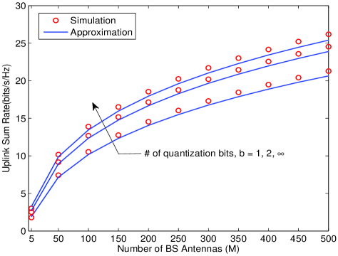
Figure 1: Uplink sum rate per cell versus the number of BS antennas, where $N=10$ users have transmit power ${p_{u}}=10$ dB.

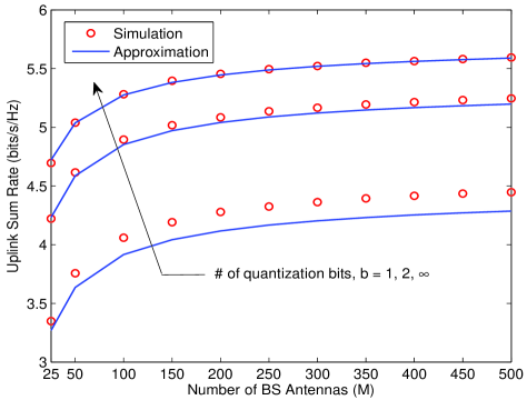
Figure 2: Uplink sum rate per cell versus the number of BS antennas, where $N=10$ users have scaled-down transmit power ${p_{u}}=\frac{E_{u}}{M}$ dB.

Finally, we illustrate energy efficiency, another important performance metric, which is defined as [9] $\eta\triangleq BR/P$ with $P={c_{0}}M{2^{b}}+{c_{1}}$, where ${c_{0}=10^{-4}}$ Watt and ${{c_{1}}=0.02}$ Watt, $B$ is the bandwidth set to 1 MHz, and $R$ is the sum rate. Given the tightness between the simulated values and approximations, we adopt the approximation in (12) for analysis. In Fig. 3, we consider the same setting as in Fig. 1, but the number of BS antennas is fixed at $M=100$. We observe that the sum rate converges to a fixed value obtained by (24). Moreover, the growth rate slows down with the increase of $b$ so that this increase also leads to significant degeneration of energy efficiency. Therefore, adopting low-resolution ADCs (e.g., $1-2$ bits) is a promising solution to ensure energy efficiency in massive MIMO systems.

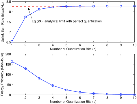
Figure 3: Uplink sum rate per cell and energy efficiency versus the number of quantization bits, where $N=10$ users have transmit power ${p_{u}}=10$ dB.

V Conclusions

We have derived a tight approximate expression for an achievable uplink rate in massive MIMO systems by using AQNM to consider the effect of ADCs. The result proves that the performance loss caused by low-resolution ADCs can be compensated by increasing the number of BS antennas, which implies the feasibility of installing low-resolution ADCs in massive MIMO systems.

References

- [1]
- [2] J. G. Andrews, S. Buzzi, C. Wan, S. V. Hanly, A. Lozano, A. C. K. Soong, J. C. Zhang, “What will 5G be?” IEEE J. Sel. Areas Commun., vol. 32, no. 6, pp. 1065-1082, Jun. 2014.
- [3] T. L. Marzetta, “Noncooperative cellular wireless with unlimited numbers of base station antennas,” IEEE Trans. Wireless Commun., vol. 9, no. 11, pp. 3590-3600, Nov. 2010.
- [4] H. Q. Ngo, E. G. Larsson, and T. L. Marzetta, “Energy and spectral efficiency of very large multiuser MIMO systems,” IEEE Trans. Commun., vol. 61, no. 4, pp. 1436-1449, Apr. 2013.
- [5] J. Singh, O. Dabeer, and U. Madhow, “On the limits of communication with low-precision analog-to-digital conversion at the receiver,” IEEE Trans. Commun., vol. 57, no. 12, pp. 3629-3639, Dec. 2009.
- [6] Q. Bai, A. Mezghani, and J. A. Nossek, “On the optimization of ADC resolution in multi-antenna systems,” in Proc. of the Tenth Int. Symposium on Wireless Commun. Systems (ISWCS 2013), pp. 1-5, Aug. 2013.
- [7] O. Orhan, E. Erkip, and S. Rangan, “Low power analog-to-digital conversion in millimeter wave systems: Impact of resolution and bandwidth on performance,” arXiv preprint arXiv: 1502.01980, available in http://arxiv.org/abs/1502.01980.
- [8] Q. Zhang, S. Jin, K. K. Wong, H. B. Zhu, and M. Matthaiou, “Power scaling of uplink massive MIMO systems with arbitrary-rank channel means,” IEEE J. Sel. Topics Signal Process., vol. 8, no. 5, pp. 966-981, Oct. 2014.
- [9] Q. Bai and J. A. Nossek, “Energy efficiency maximization for 5G multi-antenna receivers,” Trans. Emerging Tel. Tech., vol. 26, no. 1, pp. 3-14, Jan. 2015.
- [10] R. Krishnan, M. Khanzadi, N. Krishnan, Y. Wu, A. A. I. Graell, T. Eriksson, and R. Schober, “Linear massive MIMO precoders in the presence of phase noise: A Large-Scale analysis,” IEEE Trans. Veh. Tech., vol. PP, no. 99, pp. 1-1, Jan. 2015.
- [11] B. Hassibi and B. M. Hochwald, “How much training in needed in multiple-antenna wireless link?” IEEE Trans. Inf. Theory, vol. 49, no. 4, pp. 951-963, Apr. 2003.