Keldysh Field Theory for Driven Open Quantum Systems

Abstract

Recent experimental developments in diverse areas — ranging from cold atomic gases to light-driven semiconductors to microcavity arrays — move systems into the focus which are located on the interface of quantum optics, many-body physics and statistical mechanics. They share in common that coherent and driven-dissipative quantum dynamics occur on an equal footing, creating genuine non-equilibrium scenarios without immediate counterpart in equilibrium condensed matter physics. This concerns both their non-thermal stationary states, as well as their many-body time evolution. It is a challenge to theory to identify novel instances of universal emergent macroscopic phenomena, which are tied unambiguously and in an observable way to the microscopic drive conditions. In this review, we discuss some recent results in this direction. Moreover, we provide a systematic introduction to the open system Keldysh functional integral approach, which is the proper technical tool to accomplish a merger of quantum optics and many-body physics, and leverages the power of modern quantum field theory to driven open quantum systems.

I Introduction

Understanding the quantum many-particle problem is one of the grand challenges of modern physics. In thermodynamic equilibrium, the combined effort of experimental and theoretical research has made tremendous progress over the last decades, revealing the key concepts of emergent phenomena and universality. This refers to the observation, that the relevant degrees of freedom governing the macrophysics may be vastly different from those of the microscopic physics, but on the other hand are constrained by basic symmetries on the short distance scale, restoring predictive power. Regarding the role and power of these concepts in out-of-equilibrium situations, there is a large body of work in the context of classical near equilibrium and non-equilibrium many-body physics and statistical mechanics Hohenberg and Halperin (1977); Halpin-Healy and Zhang (1995); Jensen (1998); Hinrichsen (2000); Täuber (2014). However, analogous scenarios and theoretical tools for non-equilibrium quantum systems are much less developed.

This review addresses recent theoretical progress in an important and uprising class of dynamical non-equilibrium phases of quantum matter, which emerge in driven open quantum systems, where a Hamiltonian is not the only resource of dynamics. This concerns both non-equilibrium stationary states, but also the dynamics of such ensembles. Strong motivation for the exploration of non-thermal stationary states comes from a recent surge of experiments in diverse areas: in cold atomic gases Bloch et al. (2008); Lewenstein et al. (2007); Cirac and Zoller (2012), hybrid light-matter systems of Bose-Einstein condensates placed in optical cavities are created Baumann et al. (2010); Ritsch et al. (2013), or driven Rydberg ensembles are prepared Schausz et al. (2012); light-driven semiconductor heterostructures realize Bose-Einstein condensation of exciton-polaritons Kasprzak et al. (2006); Carusotto and Ciuti (2013); coupled microcavity arrays are pushed to a regime demonstrating both strong coupling of light and matter Houck et al. (2012) and scalability Underwood et al. (2012); large ensembles of trapped ions implement varieties of driven spin models Britton et al. (2012); Blatt and Roos (2012). All those systems are genuinely made of quantum ingredients, and share in common that coherent and driven-dissipative dynamics occur on equal footing. This creates close ties to typical setups in quantum optics. But on the other hand, they exhibit a continuum of degrees of freedom, characteristic for many-body physics . Systems located at this new interface are not guaranteed to thermalize, due to the absence of energy conservation and the resulting breaking of detailed balance by the external drive at the microscale. They rather converge to non-equilibrium stationary states of matter, creating scenarios without counterpart in condensed, equilibrium matter. This rules out conventional theoretical equilibrium concepts and techniques to be used, and calls for the development of new theoretical tools. The physical framework sparks broader theoretical questions on the existence of new phases of bosonic Lechner and Zoller (2013); Altman et al. (2015) and fermionic Piazza and Strack (2014a); Keeling et al. (2014); Kollath et al. (2016) matter, the nature of phase transitions in such driven systems Raftery et al. (2014); Hartmann et al. (2008); Ritsch et al. (2013); Dalla Torre et al. (2010); Sieberer et al. (2013), and the observable consequences of quantum mechanics at the largest scales van Horssen and Garrahan (2015); Marino and Diehl (2016). Beyond stationary states Hsiang and Hu (2015), a fundamental challenge is set by the time evolution of interacting quantum systems, which is currently explored theoretically Rey et al. (2004); Berges et al. (2004); Calabrese and Cardy (2006); Mitra and Giamarchi (2011); Koghee and Wouters (2014); Carusotto et al. (2010); Larré and Carusotto (2015) and experimentally in cold atomic Gring et al. (2012); Trotzky et al. (2012); Meinert et al. (2013); Hung et al. (2013); Jaskula et al. (2012) and photonic systems Nardin et al. (2009). A key goal is to identify universal dynamical regimes that hold beyond specific realizations or precise initial conditions. Combining idealized closed system evolution with the intrinsic open system character of any real world experiment takes this setting to the next stage, and exhibits emergent dynamics markedly different from closed systems both for short Buchhold and Diehl (2015a, b) and long evolution times Poletti et al. (2013); Cai and Barthel (2013); Poletti et al. (2013); Schachenmayer et al. (2014); Daley (2014); Olmos et al. (2012); Marcuzzi et al. (2014a); Lang and Piazza (2016).

The interplay of coherent and driven-dissipative dynamics can be a natural consequence of the driving necessary to maintain a certain many-body state. Going one step further, it is possible to exploit and further develop the toolbox of quantum optics for the driven-dissipative manipulation of many-body systems. Recently, it has been recognized that the concept of dissipative state preparation in quantum optics Poyatos et al. (1996); Bose et al. (1999) can be developed into a many-body context, both theoretically Diehl et al. (2008); Verstraete et al. (2009); Weimer et al. (2010); Müller et al. (2012) and experimentally Krauter et al. (2011); Barreiro et al. (2011); Schindler et al. (2013). Suitably tailored dissipation then does not necessarily act as an adversary to subtle quantum mechanical correlations such as phase coherence or entanglement Eisert and Prosen (2010); Kastoryano et al. (2011); Horstmann et al. (2013); Höning et al. (2012); Kapit et al. (2014); Lang and Büchler (2015). In contrast, it can even create these correlations, and dissipation then represents the dominant resource of many-body dynamics. In particular, even topologically ordered states in spin systems Kitaev (2006) or of fermionic matter Hasan and Kane (2010); Qi2011 can be induced dissipatively (Weimer et al. (2010) and Diehl et al. (2011); Bardyn et al. (2012); Budich et al. (2015), respectively). These developments open up a new arena for many-body physics, where the quantum mechanical microscopic origin is of key importance despite a dominantly dissipative dynamics.

Summarizing, this is a fledging topical area, where first results underpin the promise of these systems to exhibit genuinely new physics. In the remainder of the introduction, we will discuss in some more detail the three major challenges which emerge in these systems. The first one concerns the identification of novel macroscopic many-body phenomena, which witness the microscopic driven open nature of such quantum systems. Second, we anticipate the theoretical machinery, which allows us to perform the transition from micro- to macrophysics in a non-equilibrium context in practice. Third, we describe some representative experimental platforms, which motivate the theoretical efforts, and in which the predictions can be further explored.

I.1 New phenomena

As pointed out above, one of the key goals of the research reviewed here is the identification of new macroscopic many-body phenomena, which can be uniquely traced back to the microscopic driven open nature of such systems, and do not have an immediate counterpart in equilibrium systems.

The driven nature common to the systems considered here can always be associated to the fact that the underlying microscopic Hamiltonian is time dependent, with a time dependence relating to external driving fields such as lasers. When such an ensemble (i) in addition has a natural partition into a “system” and a “bath” — a continuum of modes well approximated by harmonic oscillators with short memory —, (ii) the system-bath coupling is weak compared to a typical energy scale of the “system” Hamiltonian and (iii) linear in the bath creation and annihilation operators (so that they can be integrated out straightforwardly), then an effective (still microscopic) description in terms of combined Hamiltonian and driven-dissipative Markovian quantum dynamics of the “system” ensues. The “system” dynamics obtains by tracing out the bath variables.

The resulting effective microdynamics is “non-equilibrium,” in a sense sharpened in Sec. II.4.1. This not only concerns the time evolution, but also holds for the non-equilibrium stationary states. More precisely, the above situation implies an explicit breaking of detailed balance, since the “system” energy is not conserved due to the explicitly time-dependent drive.

What do we actually mean by “detailed balance” and “thermal equilibrium?” In an operational sense, the principle of detailed balance states that there is a partition invariance for the temperature (or, more generally, the noise level) present in the system: an arbitrary bipartition of the system can be chosen, one part can be traced out, and the resulting subsystem will be at the same temperature (noise level) as the total system. This partition invariance is the condition for a globally well-defined temperature characteristic for systems in thermal equilibrium. More formally, thermal equilibrium can be detected by means of so-called fluctuation-dissipation relations (FDRs). These connect the two fundamental observables in physical systems — correlation and response functions (see Sec. II.2). In the case of thermal equilibrium, the connection is dictated by the particle statistics alone. It is then given by the Bose- and Fermi-distributions, respectively. Deviations from this universal form, which has only two free parameters (temperature and chemical potential, relating to the typical conserved quantities energy and particle number), provide a necessary requirement for non-equilibrium conditions.

In non-equilibrium stationary states, no such general form exists. We will encounter a concrete and simple example in the context of the driven Dicke model (a cavity photon coupled to a collective spin) in Sec. III.1, where the form of the FDR depends on the observable we are choosing (e.g., the position or momentum correlations and responses).

On the other hand, thermal FDRs can emerge at long wavelength, even though the microscopic dynamics manifestly breaks detailed balance Sieberer et al. (2013). In particular, in three dimensions and close to the critical point of driven-dissipative Bose-condensation, a degeneracy of critical exponents indicates a universal asymptotic thermalization, in the sense of an emergent thermal FDR. A similar phenomenology is observed in a disordered multimode extension of the Dicke model, see Sec. III.2. This underlines the strongly attractive nature of the thermal equilibrium fixed point at low frequencies. Still in these systems, non-equilibrium conditions leave their traces in the dynamical response of the system, in terms of information that does not enter the FDR at leading order. For example, the critical behavior is characterized by a fine structure in a new and independent critical exponent, which measures decoherence, and whose value distinguishes equilibrium and non-equilibrium dynamics, see Sec. IV.2.

Instead of emergent thermal behavior indicating the fadeout of non-equilibrium conditions upon coarse graining, also the opposite behavior is possible. For example, low dimensional ($d\leq 2$) bosonic systems at low noise level, such as exciton-polaritons well above threshold, are not attracted to the equilibrium fixed point as their three dimensional counterparts, but rather flow to the non-equilibrium fixed point of the Kardar-Parisi-Zhang Kardar et al. (1986) universality class, see Sec. IV.3. This can be interpreted as a universal and indefinite increase of the non-equilibrium strength, which is triggered even if the violation of detailed balance at the microscopic level is very small.

Universal non-equilibrium phenomena can also occur in the time evolution of driven open systems. For example, intriguing scaling laws describing algebraic decoherence Cai and Barthel (2013), anomalous diffusion Poletti et al. (2012), or glass-like behavior Poletti et al. (2013); Lesanovsky and Garrahan (2013, 2014); Olmos et al. (2014) have been identified in the long time asymptotics of driven spin systems close to the stationary states. Conversely, the short time behavior of driven open lattice bosons shows universal scaling laws directly witnessing the non-equilibrium drive, see Sec. V. This scaling can be related to a strongly pronounced non-equilibrium shape of the time-dependent distribution function in the early stages of evolution, and be traced back to conservation laws of the driven-dissipative generator of dynamics.

The above discussion mainly focuses on the difference between equilibrium and non-equilibrium systems on the macroscopic level of observation. Another direction, still much less developed, concerns the distinction between classical and quantum effects. Again, although the quantum mechanical description is necessary at a microscopic level, the persistence of quantum effects at the macroscale is not guaranteed. This is mainly due to the Markovian noise level inherent to such quantum systems. Nevertheless, systems with suitably engineered driven-dissipative dynamics show typical quantum mechanical phenomena such as phase coherence Diehl et al. (2008); Verstraete et al. (2009); Diehl et al. (2010a); Eisert and Prosen (2010); Horstmann et al. (2013); Höning et al. (2012), entanglement Krauter et al. (2011); Barreiro et al. (2011); Kastoryano et al. (2011); Schindler et al. (2013), or topological order Weimer et al. (2010); Diehl et al. (2011); Bardyn et al. (2012); Budich et al. (2015); Lang and Büchler (2015). Especially fermionic systems, which do not possess a classical limit, are promising in this direction.

I.2 Theoretical concepts and techniques

The development of theoretical tools needed to perform the transition from micro- to macro-physics in driven open quantum systems is still in progress, as a topic of current research. A reason for the preliminary status of the theory lies in the fact that two previously rather independent disciplines — quantum optics and many-body physics — need to be unified on a technical level.

Quantum optical systems are well described microscopically in terms of Markovian quantum master equations, which treat coherent Hamiltonian and driven-dissipative dynamics on equal footing. To solve such equations both for their dynamics and their stationary states, powerful techniques have been devised. This comprises efficient exact numerical techniques for small enough systems, such as the quantum trajectories approach Dalibard et al. (1992); Plenio and Knight (1998); Daley (2014). But it also includes analytical approaches such as perturbation theory for quantum master equations, e.g., in the frame of the Nakajima-Zwanzig projection operator technique Gardiner and Zoller (2000); Breuer and Petruccione (2002), or mappings to $P$, $W$, or $Q$ representations Carusotto and Ciuti (2005), casting the problem from a second quantized formulation into partial differential equations.

A characteristic feature of traditional quantum optical systems is the finite spacing of the few energy levels which play a role. When considering systems with a spatial continuum of degrees of freedom instead, the energy levels become continuous. This does not mean that the microscopic modelling in terms of a quantum master equation is inappropriate: for the driven-dissipative terms in such an equation, the assumption of spatially independent dissipative processes (such as atomic loss or spontaneous emission) is still valid as long as the emitted wavelength of radiation is well below the spatial resolution at the scale where the microscopic model is defined. Indeed, in this situation, destructive interference of radiation justifies the description of driven dissipation in terms of incoherent processes. However, under these circumstances the smallness of a microscopic expansion parameter no longer guarantees the smallness of the associated perturbative correction. Here the reason is that in perturbation theory, one is summing over intermediate states with propagation amplitudes down to the longest wavelengths. This can lead to infrared divergences in naive perturbation theory — a circumstance that found its physical interpretation and technical remedy in equilibrium in terms of the renormalization group Goldenfeld (1992); Cardy (1996a). We emphasize that it is precisely this situation of long wavelength dominance which underlies much of the universality, i.e., insensitivity to microscopic details, which is encountered when moving from the microscale to macroscopic observables in many-particle systems.

The modern framework to understand many-particle problems in thermodynamic equilibrium is in terms of the functional integral formulation of quantum field theory. The spectrum of its application covers a remarkable range of energy scales, from ultracold atomic gases to condensed matter systems with strong correlations to quantum chromodynamics and the quantum theory of gravity. It provides us with a well-developed toolbox of techniques, such as diagrammatic perturbation theory including sophisticated resummation schemes. But it also encompasses non-perturbative approaches, which often capitalize on the flexibility of the functional integral when it comes to picking the relevant degrees of freedom for a given problem. This is the challenge of emergent phenomena, whose solution typically is strongly scale dependent Zinn-Justin (2002). Familiar examples include an efficient description of emergent Cooper pair or molecular degrees of freedom in interacting fermion systems, or vortices which conveniently parameterize the long-wavelength physics of interacting bosons in two dimensions. The description of the change of physics with scale was given its mathematical foundation in terms of the renormalization group already mentioned above, yet another tool developed and most clearly formulated in a functional language. Finally, the functional integral based on a single scalar quantity — the system’s action, which encodes all the dynamics on the microscopic scale — is a convenient framework when it comes to the classification of symmetries and associated conservation laws, and their use in devising approximation schemes respecting them.

To put it short, while the driven open many-body systems are well described by microscopic master equations, the traditional techniques of quantum optics cannot be used efficiently – at least not in the case where the generic complications of many-body systems start to play a role. Conversely, their driven open character makes it impossible to approach these problems in the framework of equilibrium many-body physics. This situation calls for a merger of the disciplines of quantum optics and many-body physics on a technical level. On the numerical side, progress has been made in one spatial dimension recently by combining the method of quantum trajectories with powerful density matrix renormalization group algorithms Daley et al. (2009); Bernier et al. (2013); Bonnes et al. (2014); Bonnes and Läuchli (2014), see Daley (2014) for an excellent review on the topic. For more analytical approaches, the Keldysh functional or path integral Schwinger (1961, 1960); Keldysh (1965); Mahanthappa (1962); Bakshi and Mahanthappa (1963a, b) is ideally suited (but see Li et al. (2014) for a recent systematic perturbative approach to lattice Lindblad equations with extensions to sophisticated resummation schemes Li et al. (2015), and Degenfeld-Schonburg et al. (2015); Weimer (2015); Finazzi et al. (2015) for advanced variational techniques). Conceptually, the latter captures the most general situation in many-body physics — the dynamics of a density matrix under an arbitrary temporally local generator of dynamics. We refer to Kamenev (2011); Calzetta and Hu (2008) for an introduction to the Keldysh functional integral. In our context, it can be derived by a direct functional integral quantization of the Markovian quantum master equation. This procedure results in a simple translation table from the master equation to the key player in the associated Keldysh functional integral, the Markovian action. At first sight, the complexity of the non-equilibrium Keldysh functional integral is increased by the characteristic “doubling” of degrees of freedom compared to thermal equilibrium. However, it should be noted that it is precisely this feature which relates the Keldysh functional integral much closer to real time (von Neumann) evolution familiar from quantum mechanics. We will demonstrate this in Sec. II.1, making the Markovian action a rather intuitive object to work with. Furthermore, when properly harnessing symmetries, the complexity of calculations can often be made comparable to thermodynamic equilibrium. Most importantly however, the powerful toolbox of quantum field theory is opened in this way. It is thus possible to leverage the full power of sophisticated techniques from equilibrium field theory to driven open many-body systems.

Relation to classical dynamical field theories — The quantum mechanical Keldysh formulation reduces to the so-called Martin-Siggia-Rose (MSR) functional integral in the (semi-) classical limit, in turn equivalent to a stochastic Langevin equation formulation Kamenev (2011). This statement will be made precise and discussed in Sec. II.3. A large amount of work has been dedicated to this limit in the past. On the one hand, this concerns dynamical aspects of equilibrium statistical mechanics, and we refer to the classic work by Hohenberg and Halperin Hohenberg and Halperin (1977) for an overview. This work shows that, while the static universal critical behavior is determined by the symmetries and the dimensionality of the problem, the dynamical critical behavior is sensitive to additional dynamical conservation laws. This leads to a fine structure, defining dynamical universality classes which are denoted by models A–J Hohenberg and Halperin (1977). These models also provide a convenient framework to describe the statistics of work, summarized in Jarzynski’s work theorem Jarzynski (1997a, b) and Crooks’ relation Crooks (1999). On the other hand, non-equilibrium situations are captured as well. Here, we highlight in particular genuine non-equilibrium universality classes, which are not smoothly connected to the equilibrium models. Among them is the problem of reaction-diffusion models Cardy (1996b) including directed percolation Hinrichsen (2000), which is relevant to certain chemical processes (for an implementation of this universality class with driven Rydberg gases, see Marcuzzi et al. (2014a)). Another key example is surface growth, described by the Kardar-Parisi-Zhang equation Kardar et al. (1986), giving rise to a non-equilibrium universality class which is at the heart of driven phenomena such as the growth of bacterial colonies or the spreading of fire.

In the same class of approaches ranges the so-called Doi-Peliti functional integral Doi (1976); Peliti (1985), which is a functional representation of classical master equations, and may be viewed as an MSR theory with a specific, highly non-linear appearance of the field variables. It reduces to the conventional MSR form in a leading order Taylor expansion of the field non-linearities. A comprehensive overview of models, methods, and physical phenomena in the (semi-)classical limit is provided in Täuber (2014).

We also note that the usual mean field theory, where correlation functions are factorized into products of field amplitudes and which is often used as an approximation to the quantum master equation in the literature, corresponds to a further formal simplification of the semi-classical limit. Here the effects of noise are neglected completely. Conversely, the semi-classical limit represents a systematic extension of mean field theory, which includes the Markovian noise fluctuations. This level of approximation is referred to as optimal path approximation in the literature on MSR functional integrals Kamenev (2011); Täuber (2014).

In many cases, even though the microscopic description is in terms of a quantum master equation, at long distances the Keldysh field theory reduces to a semi-classical MSR field theory. The reason is the finite Markovian noise level that such systems exhibit generically, as explained in Sec. II.3. The prefix “semi” refers to the fact that phase coherence may still persist in such circumstances — the situation is comparable to a Bose-Einstein condensate at finite temperature. Recently however, situations have been identified where the drastic simplifications of the semi-classical limit do not apply. In particular, this occurs in systems with dark states — pure quantum states which are dynamical fixed points of driven-dissipative evolution Diehl et al. (2008, 2010b). In these cases, classical dynamical field theories are inappropriate, which calls for the development of quantum dynamical field theories Marino and Diehl (2016). These developments are just in their beginnings.

In this review, we concentrate on systems composed of bosonic degrees of freedom. However, it is also possible to address spin systems in terms of functional integrals Sachdev (2011), and simple models systems have been analyzed in this way, see Dalla Torre et al. (2013) and Sec. III.1. More sophisticated approaches to spin systems were elaborated in the context of multimode optical cavities in Buchhold et al. (2013), and systematically for various symmetries for lattice systems in Maghrebi and Gorshkov (2016). Fermi statistics is also conveniently implemented in the functional integral formulation. This is relevant, e.g., for driven open Fermi gases in optical cavities Keeling et al. (2014); Piazza and Strack (2014b); Kollath et al. (2016) or lattices Bernier et al. (2014), or dissipatively stabilized topological fermion matter Diehl et al. (2011); Bardyn et al. (2012); Budich et al. (2015).

I.3 Experimental platforms

The progress in controlling, manipulating, detecting and scaling up driven open quantum systems to many-body scenarios has been impressive over the last decade. Here we sketch the basic physics of three representative platforms, and indicate the relevant microscopic theoretical models in the frame of the Markovian quantum master equation. In later sections, we will translate this physics into the language of the Keldysh functional integral. For each of these platforms, excellent reviews exist, which we refer to at the end of Sec. I.4 together with further literature on open systems. The purpose of this section is to give an overview only, and to put the respective platforms into their overarching context as driven open quantum systems with many degrees of freedom.

I.3.1 Cold atoms in an optical cavity, and microcavity arrays: driven-dissipative spin-boson models

Cavity quantum electrodynamics (cavity QED), with its focus on strong light-matter interactions, is a growing field of research, which has experienced several groundbreaking advances in the past few years. Historically, these systems were developed as few or single atom experiments, detecting the radiation properties of atoms, which are strongly coupled to a quantized light field. The focus has recently been shifted towards loading more and more atoms inside a cavity. Thereby, not only single particle dynamics in strong radiation fields can be probed, but also collective, macroscopic phenomena, which are driven by light-matter interactions. For an excellent review on this topic, covering important experimental and theoretical developments, see Ritsch et al. (2013). In the experiments, cold atoms are loaded inside an optical or microwave cavity, for which the coherent interaction between the atomic internal states and a single cavity mode dominates over dissipative processes Mabuchi and Doherty (2002). The atoms absorb and emit cavity photons, thereby changing their internal states. Due to this process, the spatial modulation of the intra-cavity light field induces a coupling of the cavity photons to the atomic internal state as well as their motional degree of freedom Hood et al. (2000). In this way, cavity photons mediate an effective atom-atom interaction, which leads to a back-action of a single atom on the motion of other atoms inside the cavity. This cavity mediated interaction is long-ranged in space and represents the source of collective effects in cold atomic clouds within cavity QED experiments. One hallmark of collective dynamics in cavity QED has been the observation of self-organization of a Bose-Einstein condensate in an optical cavity. This is accompanied by a Dicke phase transition via breaking of a discrete $Z_{2}$-symmetry of the underlying model Nagy et al. (2010); Baumann et al. (2010, 2011); Maschler and Ritsch (2005).

Although the dominant dynamics in these systems is coherent, there are dissipative effects which cannot be discarded. These are the loss of cavity photons due to imperfections in the cavity mirrors, or spontaneous emission processes of atoms, which emit photons into transverse modes. These effects modify the dynamics of the system on the longest time scales. Therefore, they become relevant for macroscopic phenomena, such as phase transitions and collective dynamics. For instance, dissipative effects have been shown theoretically Öztop et al. (2012); Kulkarni et al. (2013) and experimentally Landig et al. (2015) to modify the critical exponent of the Dicke transition compared to its zero temperature value. This illustrates that for the analysis of collective phenomena in cavity QED experiments, the dissipative nature of the system has to be taken into account properly Dalla Torre et al. (2013); Brennecke et al. (2013).

Typically, for a cavity field which has a very narrow spectrum, the atomic internal degrees of freedom can be reduced to two internal states, whose transitions are nearly resonant to the photon frequency. The operators acting on these two internal states can be represented by Pauli matrices, making them equivalent to a spin-$1/2$ degree of freedom. A very important model in the framework of cavity QED is the Dicke model Hepp and Lieb (1973); Wang and Hioe (1973); Emary and Brandes (2003), which describes $N$ atoms (i.e., two-level systems) coupled to a single quantized photon mode. This is expressed by the Hamiltonian (here and in the following we set $\hbar=1$)

$$H_{\text{D}}=\omega_{0}a^{\dagger}a+\frac{\omega_{z}}{2}\sum_{i=1}^{N}\sigma^{z}_{i}+\frac{g}{\sqrt{N}}\sum_{i=1}^{N}\sigma^{x}_{i}\left(a^{\dagger}+a\right).$$ (1)

Here, $\omega_{0}$ is the photon frequency, $\sigma^{z}=|1\rangle\langle 1|-|0\rangle\langle 0|$ represents the splitting of the two atomic levels with energy difference $\omega_{z}$. $\sigma^{x}=|0\rangle\langle 1|+|1\rangle\langle 0|$ describes the coherent excitation and de-excitation of the atomic state proportional to the atom-photon coupling strength $g$. The Dicke model features a discrete $Z_{2}$ Ising symmetry: it is invariant under the transformation $(a^{\dagger},a,\sigma^{x}_{i})\mapsto(-a^{\dagger},-a,-\sigma^{x}_{i})$. In the thermodynamic limit, for $N\rightarrow\infty$, it features a phase transition, which spontaneously breaks the Ising symmetry. Crossing the transition, the system enters a superradiant phase, characterized by finite expectation values $\langle a\rangle\neq 0,\langle\sigma^{x}_{i}\rangle\neq 0$. This describes condensation of the cavity photons, i.e., the formation of a macroscopically occupied, coherent intra-cavity field, and a “ferromagnetic” ordering of the atoms in the $x$-direction.

Although the Dicke model is a standard model for cavity QED experiments in the ultra-strong coupling limit $\sqrt{N}g>\omega_{z}\omega_{0}$, it has been realized only very recently in cold atom experiments, where an entire BEC was placed inside an optical cavity Baumann et al. (2010). It has been shown that this setup maps to a Dicke model, with a “collective” spin degree of freedom Baumann et al. (2011). Here, the detuning of the pump laser was chosen such that the atoms effectively remain in the internal ground state, but acquire a characteristic recoil momentum when scattering with a cavity photon. This scattering creates a collective, motionally excited state, which replaces the role of an individual, internally excited atom. The experimental realization of a superradiance transition in the Dicke model is usually inhibited, since the required coupling strength by far exceeds the available value of the atomic dipole coupling. However, for the BEC in the cavity, the energy scales of the excited modes are much lower than the optical scale of the atomic modes. In this way, the superradiance transition indeed became experimentally accessible. This was inspired by a theoretical proposal using two balanced Raman channels between different internal atomic states inside an optical cavity, which reduced the effective level splitting of the internal states to much lower energy scales Dimer et al. (2007).

In addition to the unitary dynamics represented by the Dicke model, the cavity is subject to permanent photon loss due to imperfections in the cavity mirrors. For high finesse cavities, the coupling of the intra cavity photons to the surrounding vacuum radiation field is very weak, and the latter can be eliminated in a Born-Markov approximation Gardiner and Zoller (2000). This results in a Markovian quantum master equation for the system’s density matrix

$$\partial_{t}\rho=-i[H_{\text{D}},\rho]+\mathcal{L}_{d}\rho,$$ (2)

where $\rho$ is the density matrix for the intra cavity system and $\mathcal{L}_{d}$ adds dissipative dynamics to the coherent evolution of the Dicke model. For a vacuum radiation field, it is given by

$$\mathcal{L}_{d}\rho=\kappa\left(L\rho L^{\dagger}-\tfrac{1}{2}\{L^{\dagger}L,\rho\}\right).$$ (3)

The Lindblad operator $L$ acting on the density matrix describes pure photon loss ($L=a$) with an effective loss rate $\kappa$; the latter depends on system specific parameters, but is typically the smallest scale in the master equation (2) Ritsch et al. (2013).

In generic cavity experiments, there are also atomic spontaneous emission processes. The atoms scatter a laser or cavity photon out of the cavity, and this represents a source of decoherence. This process has been considered in Ref. Dalla Torre et al. (2013), and leads to an effective decay rate of the atomic excited state and therefore to a dephasing of the atoms, described by additional Lindblad operators $L_{i}=\sigma^{z}_{i}$ Murch et al. (2008). However, these losses are at least three orders of magnitude smaller than the cavity decay rate and typically not considered Baumann et al. (2010); Brennecke et al. (2013). The basic model for cavity QED with cold atoms is therefore represented by the Dicke model with dissipation, formulated in terms of the master equation (2). Its dynamics is discussed in Sec. III, including the Dicke superradiance transition.

The Dicke model Hamiltonian takes the form $H_{\text{D}}=H_{c}+H_{s}+H_{cs}$, where $H_{c,s,cs}$ represent the bosonic cavity, spin, and spin-boson sectors, respectively. There are many directions to go beyond the Dicke model with single collective spin, still keeping the basic feature of coupling spin to boson (cavity photon) degrees of freedom. One direction – relevant to future cold atom experiments – is to consider multimode cavities instead of a single one. In particular, in conjunction with quenched disorder, intriguing analogies to the physics of quantum glasses can be established in this way Strack and Sachdev (2011); Buchhold et al. (2013). Here, the global coupling of all spins to a single mode $g_{i}\equiv g$ is replaced by random couplings $g_{i,\ell}$, where the index $\ell$ now refers to a collection of cavity modes. The many-body physics of such an open system is discussed in Sec. III.

The basic building block of the Dicke model is the spin-boson term of the form $H_{sc}\sim(a+a^{\dagger})\sigma^{x}$, i.e. a Rabi type non-linearity that preserves the $Z_{2}$ symmetry of $H_{c,s}$. In the context of circuit quantum electrodynamics, a natural many-body generalization of Hamiltonians with a spin-boson interaction is to consider entire arrays of microcavities (instead of considering many modes within a single cavity). These cavities can be coupled to each other by single photon tunnelling processes between adjacent cavities, giving rise to Hubbard-type hopping terms $\sim Ja_{i}^{\dagger}a_{j}+\text{h. c.}$, where $i,j$ now label the spatial index of the cavities. In cirquit QED, strong non-linearities can be generated, e.g., by coupling to adjacent qubits made of Cooper pair boxes Angelakis et al. (2007); Hartmann et al. (2006). This gives rise to many-body variants of the Rabi model Schmidt and Koch (2013), whose phase diagrams have been studied recently Türeci et al. (2013); Schiró et al. (2012, 2015). Furthermore, for the implementation of lattice Dicke models with large collective spins, the use of hybrid quantum systems consisting of superconducting cavity arrays coupled to solid-state spin ensembles have been proposed Zou et al. (2014). Spontaneous collective coherence in driven-dissipative cavity arrays has been studied in Ruiz-Rivas et al. (2014).

In many physical situations (away from the ultra-strong coupling limit), a form of the spin-cavity interaction alternative to the Rabi term is more appropriate, with non-linear building block $H_{cs}\sim a\sigma^{+}+a^{\dagger}\sigma^{-}$. In fact, this form results naturally from the weak coupling rotating wave approximation of a driven spin-cavity problem. For a single cavity mode and spin, the resulting model is the Jaynes-Cummings model, which in contrast to the Dicke model possesses a continuous $U(1)$ phase rotation symmetry under $a\to e^{i\theta}a,\sigma^{-}\to e^{i\theta}\sigma^{-}$.

Clearly, when such systems are driven coherently via a Hamiltonian $H_{d}=\Omega(a+a^{\dagger})$ or suitable multimode generalizations thereof, both the $U(1)$ and even the $Z_{2}$ symmetries of the above models are broken explicitly. Coherent drive is usually the simplest way to compensate for unavoidable losses due to cavity leakage, although incoherent pumping schemes are conceivable using multiple qubits Marcos et al. (2012). An advantage of such schemes is that the symmetries of the underlying dynamics are preserved or less severely corrupted in this way (cf. the discussion in Sec. II.4). In other platforms, such as exciton-polariton systems (cf. the subsequent section), incoherent pumping is more natural from the outset.

All the systems discussed here represent genuine instances of driven open many-body systems. Besides the coherent drive, they undergo dissipative processes, which have to be taken into account for a proper understanding of their time evolution and stationary states. A generic feature of these processes is their locality. For the effective spin degrees of freedom, the typical processes are qubit decay (local Lindblad operators $L_{i}=\sigma^{-}_{i}$) and dephasing ($L_{i}=\sigma^{z}_{i}$). For the bosonic component, local single-photon loss is dominant, $L_{i}=a_{i}$.

Under various circumstances, such as a low population of the excited spin states, the latter degrees of freedom can be integrated out. In this limit, their physical effect is to generate Kerr-type bosonic non-linearities, giving rise to driven open variants of the celebrated Bose-Hubbard model. These models can even be brought into the correlation dominated regime Angelakis et al. (2007); Hartmann et al. (2006, 2008); Tomadin and Fazio (2010). Oftentimes, these approximations on the spin sector actually apply, and it is both useful and interesting to study these effective low frequency bosonic theories instead of the full many-body spin-boson problems, see Refs. Kepesidis and Hartmann (2012); Le Boité et al. (2013); Jin et al. (2014); Le Boité et al. (2014); Biella et al. (2015) for recent work in this direction.

I.3.2 Exciton-polariton systems: driven open interacting bosons

Exciton-polaritons are an extremely versatile experimental platform, which is documented by the richness of physical phenomena that have been studied in these systems both in theory and experiment. For a comprehensive account of the subject, we refer to a number of excellent review articles Carusotto and Ciuti (2013); Deng et al. (2010); Byrnes et al. (2014). A Keldysh functional integral approach is discussed in Refs. Keeling et al. (2010); Szymańska et al. (2012), which provides both a microscopic derivation of an exciton-polariton model and a mean field analysis including Gaussian fluctuations. At this point, we content ourselves with a short introduction, with the aim of showing that in a suitable parameter regime, exciton-polaritons very naturally provide a test-bed to study Bose condensation phenomena out of thermal equilibrium. Similar physics can also arise in a variety of other systems, including condensates of photons Klaers et al. (2010), magnons Demokritov et al. (2006), and potentially excitons Alloing et al. (2014). Remarkably, even cold atoms could be brought to condense in a non-equilibrium regime, where continuous loading of atoms balances three-body losses Falkenau et al. (2011), or in atom laser setups Mewes et al. (1997); Robins et al. (2008, 2013).

A basic experimental setup for exciton-polaritons consists of a planar semiconductor microcavity embedding a quantum well (see Fig. 1 (a)). This setting allows for a strong coupling of cavity light and matter in the quantum well, as originally proposed in Imamoglu et al. (1996). The free dynamics of the elementary excitations of this system — i.e., of cavity photons and Wannier-Mott excitons — is described by the quadratic Hamiltonian Carusotto and Ciuti (2013)

$$H_{0}=H_{C}+H_{X}+H_{\mathit{C-X}},$$ (4)

where the parts of the Hamiltonian involving only photons and excitons, respectively, take the same form, which is given by (here the index $\alpha$ labels cavity photons, $\alpha=C$, and excitons, $\alpha=X$, respectively)

$$H_{\alpha}=\int\frac{d\mathbf{q}}{\left(2\pi\right)^{2}}\sum_{\sigma}\omega_{\alpha}(q)a_{\alpha,\sigma}^{\dagger}(\mathbf{q})a_{\alpha,\sigma}(\mathbf{q}).$$ (5)

Field operators $a_{\alpha,\sigma}^{\dagger}(\mathbf{q})$ and $a_{\alpha,\sigma}(\mathbf{q})$ create or destroy a photon or exciton (note that both are bosonic excitations) with in-plane momentum $\mathbf{q}$ and polarization $\sigma$ (there are two polarization states of the exciton which are coupled to the cavity mode Carusotto and Ciuti (2013)). For simplicity, we neglect polarization effects leading to an effective spin-orbit coupling Carusotto and Ciuti (2013). Due to the confinement in the transverse ($z$) direction, i.e., along the cavity axis, the motion of photons in this direction is quantized as $q_{z,n}=\pi n/l_{z}$, where $n$ is a positive integer, and $l_{z}$ is the length of the cavity. In writing the Hamiltonian (5), we are assuming that only the lowest transverse mode is populated, which leads to a quadratic dispersion as a function of the in-plane momentum $q=\left\lvert\mathbf{q}\right\rvert=\sqrt{q_{x}^{2}+q_{y}^{2}}$:

$$\omega_{C}(q)=c\sqrt{q_{z,1}^{2}+q^{2}}=\omega_{C}^{0}+\frac{q^{2}}{2m_{C}}+O(q^{4}).$$ (6)

Here, $c$ is the speed of sound, $\omega_{C}^{0}=cq_{z,1}$, and the effective mass of the photon is given by $m_{C}=q_{z,1}/c$. Typically, the value of the photon mass is orders of magnitude smaller than the mass of the exciton, so that the dispersion of the latter appears to be flat on the scale of Fig. 1 (b).

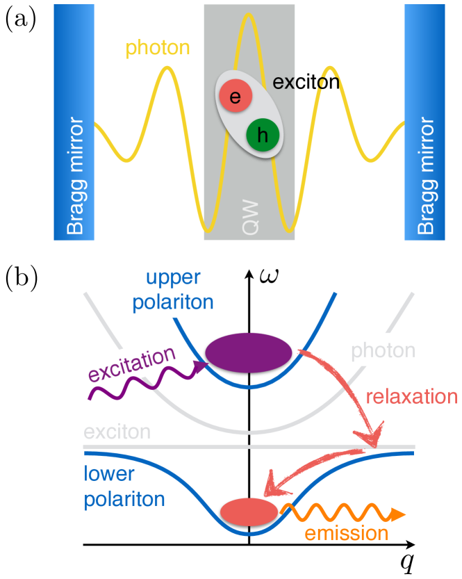
Figure 1: (a) Schematic of two Bragg mirrors forming a microcavity, in which a quantum well (QW) is embedded. In the regime of strong light-matter interaction, the cavity photon and the exciton hybridize and form new eigenmodes, which are called exciton-polaritons. (b) Energy dispersion of the upper and lower polariton branches as a function of in-plane momentum $q$. In the experimental scheme illustrated in this figure (cf. Ref. Kasprzak et al. (2006)), the incident laser is tuned to highly excited states of the quantum well. These undergo relaxation via emission of phonons and scattering from polaritons, and accumulate at the bottom of the lower polariton branch. In the course of the relaxation process, coherence is quickly lost, and the effective pumping of lower polaritons is incoherent.

Upon absorption of a photon by the semiconductor, an exciton is generated. This process (and the reverse process of the emission of a photon upon radiative decay of an exciton) is described by

$$H_{\mathit{C-X}}=\Omega_{R}\int\frac{d\mathbf{q}}{\left(2\pi\right)^{2}}\sum_{\sigma}\left(a_{X,\sigma}^{\dagger}(\mathbf{q})a_{C,\sigma}(\mathbf{q})+\mathrm{H.c.}\right),$$ (7)

where $\Omega_{R}$ is the rate of the coherent interconversion of photons into excitons and vice versa. The quadratic Hamiltonian (4) can be diagonalized by introducing new modes — the lower and upper exciton-polaritons, $\psi_{\mathrm{LP},\sigma}(\mathbf{q})$ and $\psi_{\mathrm{UP},\sigma}(\mathbf{q})$ respectively, which are linear combinations of photon and exciton modes. The dispersion of lower and upper polaritons is depicted in Fig. 1 (b). In the regime of strong light-matter coupling, which is reached when $\Omega_{R}$ is larger than both the rate at which photons are lost from the cavity due to mirror imperfections and the non-radiative decay rate of excitons, it is appropriate to think of exciton-polaritons as the elementary excitations of the system.

In experiments, it is often sufficient to consider only lower polaritons in a specific spin state, and to approximate the dispersion as parabolic Carusotto and Ciuti (2013). Interactions between exciton-polaritons originate from various physical mechanisms, with a dominant contribution stemming from the screened Coulomb interactions between electrons and holes forming the excitons. Again, in the low-energy scattering regime, this leads to an effective contact interaction between lower polaritons. As a result, the low-energy description of lower polaritons takes the form (in the following we drop the subscript indices in $\psi_{\mathrm{LP},\sigma}$) Carusotto and Ciuti (2013)

$$H_{\mathrm{LP}}=\int d\mathbf{x}\left[\psi^{\dagger}(\mathbf{x})\left(\omega_{\mathrm{LP}}^{0}-\frac{\nabla^{2}}{2m_{\mathrm{LP}}}\right)\psi(\mathbf{x})+u_{c}\psi^{\dagger}(\mathbf{x})^{2}\psi(\mathbf{x})^{2}\right].$$ (8)

While this Hamiltonian is quite generic and arises also, e.g., in cold bosonic atoms in the absence of an external potential, the peculiarity of exciton-polaritons is that they are excitations with relatively short lifetime. In turn, this necessitates continuous replenishment of energy in the form of laser driving in order to maintain a steady population. In Fig. 1 (b), we consider the case in which the excitation laser is tuned to energies well above the lower polariton band. The thus created high-energy excitations are deprived of their excess energy via phonon-polariton and stimulated polariton-polariton scattering. Eventually, they accumulate at the bottom of the lower polariton band. As a consequence of multiple scattering processes, the coherence of the incident laser field is quickly lost, and the effective pumping of lower polaritons is incoherent.

A phenomenological model for the dynamics of the lower polariton field, which accounts for both the coherent dynamics generated by the Hamiltonian (8) and the driven-dissipative one described above, was introduced in Ref. Wouters and Carusotto (2007a). It involves a dissipative Gross-Pitaevskii equation for the lower polariton field that is coupled to a rate equation for the reservoir of high-energy excitations. However, for the study of universal long-wavelength behavior in Sec. IV, this degree of microscopic modeling is actually not required: indeed, any (possibly simpler) model that possesses the relevant symmetries (see the discussion at the beginning of Sec. IV) will yield the same universal physics. Such a model can be obtained by describing incoherent pumping and losses of lower polaritons by means of a Markovian master equation:

$$\partial_{t}\rho=-i[H_{\mathrm{LP}},\rho]+\mathcal{L}_{d}\rho,$$ (9)

where $\mathcal{L}_{d}\rho$ encodes incoherent single-particle pumping and losses, as well as two-body losses:

$$\mathcal{L}_{d}\rho=\int d\mathbf{x}\left(\gamma_{p}\mathcal{D}[\psi(\mathbf{x})^{\dagger}]\rho+\gamma_{l}\mathcal{D}[\psi(\mathbf{x})]\rho+2u_{d}\mathcal{D}[\psi(\mathbf{x})^{2}]\rho\right),$$ (10)

where

$$\mathcal{D}[L]\rho=L\rho L^{\dagger}-\frac{1}{2}\{L^{\dagger}L,\rho\}$$ (11)

reflects the Lindblad form, and $\gamma_{p}$, $\gamma_{l}$, $2u_{d}$ are the rates of single-particle pumping, single-particle loss, and two-body loss, respectively. The inclusion of the non-linear loss term ensures saturation of the pumping. An analogous mechanism is implemented in the above-mentioned Gross-Pitaevskii description. More precisely, in the spirit of universality, the above quantum master equation  (9) and the above mentioned phenomenological model reduce to precisely the same low frequency model for bosonic degrees of freedom upon taking the semiclassical limit in the Keldysh path integral associated to Eq. (9) (see Sec. II.3 for its implementation), and integrating out the upper polariton reservoir in the phenomenological model.

I.3.3 Cold atoms in optical lattices: heating dynamics

In recent years, experiments with cold atoms in optical lattices have shown remarkable progress in the simulation of many-body model systems both in and out of equilibrium. A particular strength of cold atom experiments is the unprecedented tuneability of model parameters, such as the local interaction strength and the lattice hopping amplitude. This becomes possible by, e.g., manipulation of the lattice laser and external magnetic fields. It comes along with a very weak coupling of the system to the environment, such that the dynamics can often be seen as isolated on relevant time scales for typical measurements of static, equilibrium correlations. However, more and more experiments start to investigate the realm of non-equilibrium phenomena with cold atoms, e.g., by letting systems prepared in a non-equilibrium initial condition relax in time towards a steady state Hackermüller et al. (2010); Meinert et al. (2013, 2014); Gring et al. (2012); Preiss et al. (2015). With these experiments, time scales are reached, for which the dissipative coupling to the environment becomes visible in experimental observables. Such dissipation may even hinder the system from relaxation towards a well defined steady state.

A relevant example of a dissipative coupling is decoherence of an atomic cloud induced by spontaneous emission of atoms in the lattice Pichler et al. (2010, 2013). In this way, the many-body system is heated up, and therefore driven away from the low entropy state in which it was prepared initially. A detailed discussion of the microscopic physics and its long time dynamics can be found in Schachenmayer et al. (2014); Poletti et al. (2013); Cai and Barthel (2013), see also the review article Daley (2014). For bosonic atoms in optical lattices, the coherent dynamics is described by the Bose-Hubbard Hamiltonian Fisher et al. (1989); Jaksch et al. (1998)

$$H_{\text{BH}}=-J\sum_{\langle l,m\rangle}b^{\dagger}_{l}b_{m}+\frac{U}{2}\sum_{l}n_{l}(n_{l}-1),$$ (12)

which models bosonic atoms in terms of the creation and annihilation operators $[b^{\phantom{\dagger}}_{l},b^{\dagger}_{m}]=\delta_{lm}$ in the lowest band of a lattice with site indices $l,m$. The atoms hop between neighboring lattice sites with an amplitude $J$, and experience an on-site repulsion $U$. The lattice potential $V(x)$, which leads to the second quantized form of the Bose-Hubbard model, is created by the superposition of counter-propagating laser beams in each spatial dimension. The coherent laser field couples two internal atomic states via stimulated absorption and emission, which leads to the single particle Hamiltonian

$$H_{\text{atom}}=\frac{\hat{\bf p}^{2}}{2m}-\frac{\Delta}{2}\sigma^{z}-\sigma^{x}\frac{\Omega(\hat{\bf x})}{2},$$ (13)

where $\hat{\bf p}$ is the atomic momentum operator, $\Delta$ is the detuning of the laser from the atomic transition frequency, and $\Omega(\hat{\bf x})$ is the laser field at the atomic position. For large detuning, the excited state of the atom can be traced out, which leads to the lattice Hamiltonian

$$H_{\text{atom}}^{\text{eff}}=\frac{\hat{\bf p}^{2}}{2m}+\frac{|\Omega(\hat{\bf x})|^{2}}{4\Delta}.$$ (14)

This describes a lattice potential for the ground state atoms generated by the spatially modulated AC Stark shift. Adding an atomic interaction potential and expanding both the single particle Hamiltonian (14) and the interaction in terms of Wannier states, the leading order Hamiltonian is the Bose-Hubbard model (12) Jaksch et al. (1998).

In the semi-classical treatment of the atom-laser interaction, spontaneous emission events are neglected, as their probability is typically very small (see below for a more precise statement). They can be taken into account on the basis of optical Bloch equations Pichler et al. (2010), which leads, after elimination of the excited atomic state, to an additional, driven-dissipative term in the atomic dynamics. It describes the decoherence of the atomic state due to spontaneous emission, i.e., position dependent random light scattering. The leading order contribution to the dynamics in the basis of lowest band Wannier states is captured by the master equation

$$\partial_{t}\rho=-i[H_{\text{BH}},\rho]-\gamma\sum_{l}[n_{l},[n_{l},\rho]],$$ (15)

where $n_{l}=b^{\dagger}_{l}b^{\phantom{\dagger}}_{l}$ is the local atomic density, and $\rho$ is the many-body density matrix. For a red detuned laser the rate $\gamma=\Gamma\frac{|\Omega|^{2}}{4\Delta^{2}}$ is proportional to the microscopic spontaneous emission rate $\Gamma$ and the laser amplitude $|\Omega|$. Note the suppression of the scale $\gamma$ by a factor $\Gamma/\Delta\ll 1$ for large detuning, compared to the strength of $H_{\text{atom}}^{\text{eff}}$. The coherent and incoherent contribution of the atom-laser coupling to the dynamics is illustrated in Fig. 2.

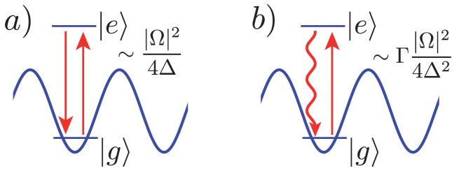
Figure 2: Illustration of the coherent (a) and the incoherent (b) contribution to the dynamics stemming from the coupling of the atoms to a laser with amplitude $|\Omega|$ and large detuning $\Delta$. (a) Via the AC Stark effect, stimulated absorption and emission lead to a coherent periodic potential with amplitude $\frac{|\Omega|^{2}}{4\Delta}$. (b) Stimulated absorption and subsequent spontaneous emission lead to effective decoherence of the atomic state with rate $\Gamma\frac{|\Omega|^{2}}{4\Delta}$, where $\Gamma$ is the microscopic spontaneous emission rate.

The dissipative term in the master equation (15) leads to an energy increase $\langle H_{\text{BH}}\rangle(t)\sim t$ linear in time, and thus to heating. Furthermore, it introduces decoherence in the number state basis, i.e., it projects the local density matrix on its diagonal in Fock space and leads to a decrease of the coherences in time Daley (2014); Schachenmayer et al. (2014); Poletti et al. (2013); Cai and Barthel (2013). Starting from a low entropy state at $t=0$, the heating leads to a crossover from coherence dominated dynamics at short and intermediate times Buchhold and Diehl (2015a) to a decoherence dominated dynamics at long times Schachenmayer et al. (2014); Poletti et al. (2013); Cai and Barthel (2013). In one dimension, both regimes have been analyzed extensively both numerically (with a focus on decoherence dominated dynamics) as well as analytically, and display several aspects of non-equilibrium universality, see Sec. V. Therefore, heating in interacting lattice systems represents a crucial example for universality in out-of-equilibrium dynamics, which can be probed by cold atom experiments.

I.4 Outline and scope of this review

The remainder of this review is split into two parts.

Part 1 develops the theoretical framework for the efficient description of driven open many-body quantum systems. In Sec. II, we begin with a direct derivation of the open system Keldysh functional integral from the many-body quantum master equation (Sec. II.1). We then discuss in Sec. II.2.1 in detail a simple example: the damped and driven optical cavity. This allows the reader to familiarize with the functional formalism. In particular, the key players in terms of observables — correlation and response functions — are described. We also point out a number of exact structural properties of Keldysh field theories, which hold beyond the specific example. Another example is introduced in Sec. II.2.2: there we discuss the mean field theory of condensation in a bosonic many-body system with particle losses and pumping. The semi-classical limit of this model and its validity are the content of Sec. II.3. This is followed by a discussion of symmetries and conservation laws in the Keldysh formalism in Sec. II.4. In particular, we point out a symmetry that allows one to distinguish equilibrium from non-equilibrium conditions. Finally, an advanced field theoretical tool — the open system functional renormalization group — is introduced in Sec. II.5.

Part 2 harnesses this formalism to generate an understanding of the physics in different experimental platforms. We begin in Sec. III with simple but paradigmatic spin models with discrete Ising $Z_{2}$ symmetry in driven non-equilibrium stationary states. In particular, we discuss the physics of the driven open Dicke model in Sec. III.1. This is followed by an extended variant of the latter in the presence of disorder and a multimode cavity, which hosts an interesting spin and photon glass phase in Sec. III.2. Sec. IV is devoted to the non-equilibrium stationary states of bosons with a characteristic $U(1)$ phase rotation symmetry: the driven-dissipative condensates introduced in Sec. II.2.2. After some additional technical developments relating to $U(1)$ symmetry in Sec. IV.1, we discuss critical behavior at the Bose condensation transition in three dimensions. In particular, we show the decrease of a parameter quantifying non-equilibrium strength in this case (Sec. IV.2). The opposite behavior is observed in two (Sec. IV.3) and one (Sec. IV.4) dimensions. Finally, leaving the realm of stationary states, in Sec. V we discuss an application of the Keldysh formalism to the time evolution of open bosonic systems in one dimension, which undergo number conserving heating processes. We set up the model in Sec. V.1, derive the kinetic equation for the distribution function in Sec. V.2, and discuss the relevant approximations and physical results in Secs. V.3 and V.4, respectively. Conclusions are drawn in Sec. VI. Finally, brief introductions to functional differentiation and Gaussian functional integration are given in Appendices A and B.

Reflecting the bipartition of this review, the scope of it is twofold. On the one hand, it develops the Keldysh functional integral approach to driven open quantum systems “from scratch”, in a systematic and coherent way. It starts from the Markovian quantum master equation representation of driven dissipative quantum dynamics Gardiner and Zoller (2000); Breuer and Petruccione (2002); Barnett and Radmore (1997), and introduces an equivalent Keldysh functional integral representation. Direct contact is made to the language and typical observables of quantum optics. It does not require prior knowledge of quantum field theory, and we hope that it will find the interest of — and be useful for — researchers working on quantum optical systems with many degrees of freedom. On the other hand, this review documents some recent theoretical progresses made in this conceptual framework in a more pedagogical way than the original literature. We believe that this not only exposes some interesting physics, but also demonstrates the power and flexibility of the Keldysh approach to open quantum systems.

This work is complemetary to excellent reviews putting more emphasis on the specific experimental platforms partially mentioned above: The physics of driven Bose-Einstein condensates in optical cavities is reviewed in Ritsch et al. (2013). A general overview of driven ultracold atomic systems, specifically in optical lattices, is provided in Daley (2014), and systems with engineered dissipation are described in Müller et al. (2012). Detailed accounts for exciton-polariton systems are given in Carusotto and Ciuti (2013); Deng et al. (2010); Byrnes et al. (2014); specifically, we refer to the review Keeling et al. (2010) working in the Keldysh formalism. The physics of microcavity arrays is discussed in Hartmann et al. (2008); Tomadin and Fazio (2010); Houck et al. (2012); Schmidt and Koch (2013), and trapped ions are treated in Leibfried et al. (2003); Blatt and Roos (2012). We also refer to recent reviews on additional upcoming platforms of driven open quantum systems, such as Rydberg atoms Marcuzzi et al. (2014b) and opto-nanomechanical settings Marquardt and Girvin (2009). For a recent exposition of the physics of quantum master equations and to efficient numerical techniques for their solution, see Daley (2014).

Part 1 Theoretical background

II Keldysh functional integral for driven open systems

In this part, we will be mainly concerned with a Keldysh field theoretical reformulation of the stationary state of Markovian many-body quantum master equations. As we also demonstrate, this opens up the powerful toolbox of modern quantum field theory for the understanding of such systems.

The quantum master equation, examples of which we have already encountered in Sec. I.3, describes the time evolution of a reduced system density matrix $\rho$ and reads Gardiner and Zoller (2000); Breuer and Petruccione (2002)

$$\partial_{t}\rho=\mathcal{L}\rho=-i[H,\rho]+\sum_{\alpha}\gamma_{\alpha}\left(L_{\alpha}\rho L_{\alpha}^{\dagger}-\frac{1}{2}\{L_{\alpha}^{\dagger}L_{\alpha},\rho\}\right),$$ (16)

where the operator $\mathcal{L}$ acts on the density matrix $\rho$ “from both sides” and is often referred to as Liouville superoperator or Liouvillian (sometimes this term is reserved for the second contribution on the RHS of Eq. (16) alone). There are two contributions to the Liouvillian: first, the commutator term, which is familiar from the von Neumann equation, describes the coherent dynamics generated by a system Hamiltonian $H$; the second part, which we will refer to as the dissipator $\mathcal{D}$ , describes the dissipative dynamics resulting from the interaction of the system with an environment, or “bath.” It is defined in terms of a set of so-called Lindblad operators (or quantum jump operators) $L_{\alpha}$, which model the coupling to that bath. The dissipator has a characteristic Lindblad form Lindblad (1976); Kossakowski (1972): it contains an anticommutator term which describes dissipation; in order to conserve the norm $\mathop{\mathrm{tr}}(\rho)$ of the system density matrix, this term must be accompanied by fluctuations. The corresponding term, where the Lindblad operators act from both sides onto the density matrix, is referred to as recycling or quantum jump term. Dissipation occurs at rates $\gamma_{\alpha}$ which are non-negative, so that the density matrix evolution is completely positive, i.e., the eigenvalues of $\rho$ remain positive under the combined dynamics generated by $H$ and $\mathcal{D}$ Bacon et al. (2001). If the index $\alpha$ is the site index in an optical lattice or in a microcavity array, or even a continuous position label (in which case the sum is replaced by an integral), in a translation invariant situation there is just a single scale $\gamma_{\alpha}=\gamma$ for all $\alpha$ associated to the dissipator.

The quantum master equation (16) provides an accurate description of a system-bath setting with a strong separation of scales. This is generically the case in quantum optical systems, which are strongly driven by external classical fields. More precisely, there must be a large energy scale in the bath (as compared to the system-bath coupling), which justifies to integrate out the bath in second-order time-dependent perturbation theory. If in addition the bath has a broad bandwidth, the combined Born-Markov and rotating-wave approximations are appropriate, resulting in Eq. (16). A concrete example for such a setting is provided by a laser-driven atom undergoing spontaneous emission. Generic condensed matter systems do not display such a scale separation, and a description in terms of a master equation of the type (16) is not justified. However, the systems discussed in the introduction, belong to the class of systems which permit a description by Eq. (16). We refer to them as driven open many-body quantum systems.

Due to the external drive these systems are out of thermodynamic equilibrium. This statement will be made more precise in Sec. II.4.1 in terms of the absence of a dynamical symmetry which characterizes any system evolving in thermodynamic equilibrium, and which is manifestly violated in dynamics described by Eq. (16). Its absence reflects the lack of energy conservation and the epxlicit breaking of detailed balance. As stated in the introduction, the main goal of this review is to point out the macroscopic, observable consequences of this microscopic violation of equilibrium conditions.

II.1 From the quantum master equation to the Keldysh functional integral

In this section, starting from a many-body quantum master equation Eq. (16) in the operator language of second quantization, we derive an equivalent Keldysh functional integral. We focus on stationary states, and we discuss how to extract dynamics from this framework in Sec. V. Our derivation of the Keldysh functional integral applies to a theory of bosonic degrees of freedom. If spin systems are to be considered, it is useful to first perform the typical approximations mapping them to bosonic fields, and then proceed along the construction below (see Sec. III and Refs. Dalla Torre et al. (2013); Maghrebi and Gorshkov (2016)). Clearly, this amounts to an approximate treatment of the spin degrees of freedom; for an exact (equilibrium) functional integral representation for spin dynamics, taking into account the full non-linear structure of their commutation relations, we refer to Ref. Altland and Simons (2010). For fermionic problems, the construction is analogous to the bosonic case presented here. However, a few signs have to be adjusted to account for the fermionic anticommutation relations Altland and Simons (2010); Kamenev (2011).

The basic idea of the Keldysh functional integral can be developed in simple terms by considering the Schrödinger vs. the von Neumann equation,

$$i\partial_{t}|\psi(t)\rangle =H|\psi(t)\rangle \Rightarrow |\psi(t)\rangle =U(t,t_{0})|\psi(t_{0})\rangle,$$

$$\partial_{t}\rho(t) =-i[H,\rho(t)] \Rightarrow \rho(t) =U(t,t_{0})\rho(t_{0})U^{\dagger}(t,t_{0}),$$ (17)

where $U(t,t_{0})=e^{-iH\left(t-t_{0}\right)}$ is the unitary time evolution operator. In the first case, a real time path integral can be constructed along the lines of Feynman’s original path integral formulation of quantum mechanics Feynman (1948). To this end, a Trotter decomposition of the evolution operator

$$e^{-iH\left(t-t_{0}\right)}=\lim_{N\rightarrow\infty}\left(\mathbbm{1}-i\delta_{t}H\right)^{N},$$ (18)

with $\delta_{t}=\frac{t-t_{0}}{N}$, is performed. Subsequently, in between the factors of the Trotter decomposition, completeness relations in terms of coherent states are inserted in order to make the (normal ordered) Hamilton operator a functional of classical field variables. This is illustrated in Fig. 3 a), and we will perform these steps explicitly and in more detail below in the context of open many-body systems. Crucially, we only need one set of field variables representing coherent Hamiltonian dynamics, which corresponds to the forward evolution of the Schrödinger state vector. It is also clear that — noting the formal analogy of the operators $e^{-iH\left(t-t_{0}\right)}$ and $e^{-\beta H}$ — this construction can be leveraged over to the case of thermal equilibrium, where the “Trotterization” is done in imaginary instead of real time.

In contrast to these special cases, the von Neumann equation for general mixed state density matrices cannot be rewritten in terms of a state vector evolution, even in the case of purely coherent Hamiltonian dynamics. Instead, it is necessary to study the evolution of a state matrix, which transforms according to the integral form of the von Neumann equation in the second line of Eq. (II.1). Therefore, we have to apply the Trotter formula and coherent state insertions on both sides of the density matrix. This leads to the doubling of degrees of freedom, characteristic of the Keldysh functional integral. Moreover, time evolution can now be interpreted as occurring along two branches, which we denote as the forward and a backward branches, respectively (cf. Fig. 3 b)). Indeed, this is an intuitive and natural feature of evolving matrices instead of vectors.

So far, we have concentrated on closed systems which evolve according to purely Hamiltonian dynamics. However, we can allow for a more general generator of dynamics and still proceed along the two-branch strategy. The most general (time local) evolution of a density matrix is given by the quantum master equation (16). Its formal solution reads

$$\rho(t)=e^{\left(t-t_{0}\right)\mathcal{L}}\rho(t_{0})\equiv\lim_{N\rightarrow\infty}\left(\mathbbm{1}+\delta_{t}\mathcal{L}\right)^{N}\rho(t_{0}).$$ (19)

The last equality gives a meaning to the formal solution in terms of the Trotter decomposition: at each infinitesimal time step, the exponential can be expanded to first order, such that the action of the Liouvillian superoperator is just given by the RHS of the quantum master equation (16); At finite times, the evolved state is given by the concatenation of the infinitesimal Trotter steps.

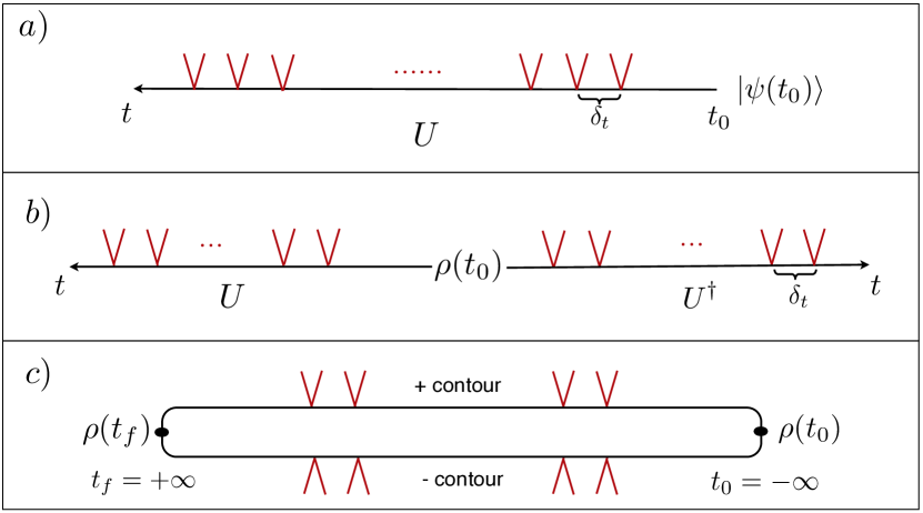
Figure 3: Idea of the Keldysh functional integral. a) According to the Schrödinger equation, the time evolution of a pure state vector is described by the unitary operator $U(t,t_{0})=e^{-iH\left(t-t_{0}\right)}$. In the Feynman functional integral construction, the time evolution is chopped into infinitesimal steps of length $\delta_{t}$, and completeness relations in terms of coherent states are inserted in between consecutive time steps. This insertion is signalled by the red arrows. b) In contrast, if the state is mixed, a density matrix must be evolved, and thus two time branches are needed. As explained in the text, the dynamics need not necessarily be restricted to unitary evolution. The most general time-local (Markovian) dynamics is generated by a Liouville operator in Lindblad form. c) For the analysis of the stationary state, we are interested in the real time analog of a partition function $Z=\mathop{\mathrm{tr}}\rho(t_{f})$, starting from $t_{0}=-\infty$ and running until $t_{f}=+\infty$. The trace operation connects the two time branches, giving rise to the closed Keldysh contour.

If we restrict ourselves to the stationary state of the system, but want to evaluate correlations at arbitrary time differences, we should extend the time branch from an initial time in the distant past $t_{0}\to-\infty$ to the distant future, $t_{f}\to+\infty$. In analogy to thermodynamics, we are then interested in the so-called Keldysh partition function $Z=\mathop{\mathrm{tr}}\rho(t)=1$. The trace operation contracts the indices of the time evolution operator as depicted in Fig. 3 c), giving rise to the closed time path or Keldysh contour. Conservation of probability in the quantum mechanical system is reflected in the time-independent normalization of the partition function. In order to extract physical information, again in analogy to statistical mechanics, below we introduce sources in the partition function. This allows us to compute the correlation and response functions of the system by taking suitable variational derivatives with respect to the sources.

After this qualitative discussion, let us now proceed with the explicit construction of the Keldysh functional integral for open systems, starting from the master equation (16). As mentioned above, the Keldysh functional integral is an unraveling of Liouvillian dynamics in the basis of coherent states, and we first collect a few important properties of those. Coherent states are defined as (for simplicity, in the present discussion we restrict ourselves to a single bosonic mode $b$) $\ket{\psi}=\exp(\psi b^{\dagger})\ket{\Omega}$, where $\ket{\Omega}$ represents the vacuum in Fock space. (Note that according to this definition, which is usually adopted in the discussion of field integrals Negele and Orland (1998), the state $\ket{\psi}$ is not normalized.) A key property of coherent states is that they are eigenstates of the annihilation operator, i.e., $b\ket{\psi}=\psi\ket{\psi}$, with the complex eigenvalue $\psi$. Clearly, this implies the conjugate relation $\bra{\psi}b^{\dagger}=\bra{\psi}\psi^{*}$. The overlap of two non-normalized coherent states is given by $\braket{\psi}{\phi}=e^{\psi^{*}\phi}$, and the completeness relation reads $\mathbbm{1}=\int\frac{d\psi d\psi^{*}}{\pi}e^{-\psi^{*}\psi}\ket{\psi}\bra{\psi}$.

The starting point of the derivation is Eq. (19), and we focus first on a single time step, as in the usual derivation of the coherent state functional integral Negele and Orland (1998). That is, we decompose the time evolution from $t_{0}$ to $t_{f}$ into a sequence of small steps of duration $\delta_{t}=(t_{f}-t_{0})/N$, and denote the density matrix after the $n$-th step, i.e., at the time $t_{n}=t_{0}+\delta_{t}n$, by $\rho_{n}=\rho(t_{n})$. We then have

$$\rho_{n+1}=e^{\delta_{t}\mathcal{L}}\rho_{n}=\left(\mathbbm{1}+\delta_{t}\mathcal{L}\right)\rho_{n}+O(\delta_{t}^{2}).$$ (20)

As anticipated above, we proceed to represent the density matrix in the basis of coherent states. For instance, $\rho_{n}$ at the time $t_{n}$ can be written as

$$\rho_{n}=\int\frac{d\psi_{+,n}d\psi_{+,n}^{*}}{\pi}\frac{d\psi_{-,n}d\psi_{-,n}^{*}}{\pi}e^{-\psi_{+,n}^{*}\psi_{+,n}-\psi_{-,n}^{*}\psi_{-,n}}\\ \times\braket{\psi_{+,n}}{\rho_{n}}{\psi_{-,n}}\ket{\psi_{+,n}}\bra{\psi_{-,n}}.$$ (21)

As a next step, we would like to express the matrix element $\braket{\psi_{+,n+1}}{\rho_{n+1}}{\psi_{-,n+1}}$, which appears in the coherent state representation of $\rho_{n+1}$, in terms of the corresponding matrix element at the previous time step $t_{n}$. Inserting Eq. (21) in Eq. (20), we find that this requires us to evaluate the “supermatrixelement”

$$\braket{\psi_{+,n+1}}{\mathcal{L}(\ket{\psi_{+,n}}\bra{\psi_{-,n}})}{\psi_{-,n+1}}=-i\left(\braket{\psi_{+,n+1}}{H}{\psi_{+,n}}\braket{\psi_{-,n}}{\psi_{-,n+1}}-\braket{\psi_{+,n+1}}{\psi_{+,n}}\braket{\psi_{-,n}}{H}{\psi_{-,n+1}}\right)\\ +\sum_{\alpha}\gamma_{\alpha}\left[\braket{\psi_{+,n+1}}{L_{\alpha}}{\psi_{+,n}}\braket{\psi_{-,n}}{L_{\alpha}^{\dagger}}{\psi_{-,n+1}}-\frac{1}{2}\left(\braket{\psi_{+,n+1}}{L_{\alpha}^{\dagger}L_{\alpha}}{\psi_{+,n}}\braket{\psi_{-,n}}{\psi_{-,n+1}}+\braket{\psi_{+,n+1}}{\psi_{+,n}}\braket{\psi_{-,n}}{L_{\alpha}^{\dagger}L_{\alpha}}{\psi_{-,n+1}}\right)\right].$$ (22)

Without loss of generality, we assume that the Hamiltonian is normal ordered. Then, a matrix element $\braket{\psi}{H}{\phi}$ of the Hamiltonian between coherent states can be obtained simply by replacing the creation operators by $\psi^{*}$ and the annihilation operators by $\phi$. The same is true for matrix elements of $L,L^{\dagger},$ and $L^{\dagger}L$, after performing the commutations which are necessary to bring these operators to the form of sums of normal ordered expressions (see Ref. Sieberer et al. (2014) for a detailed discussion of subtleties related to normal ordering). Then we obtain by re-exponentiation

$$\braket{\psi_{+,n+1}}{\rho_{n+1}}{\psi_{-,n+1}}=\int\frac{d\psi_{+,n}d\psi_{+,n}^{*}}{\pi}\frac{d\psi_{-,n}d\psi_{-,n}^{*}}{\pi}e^{i\delta_{t}\left(-\psi_{+,n}i\partial_{t}\psi_{+,n}^{*}-\psi_{-,n}^{*}i\partial_{t}\psi_{-,n}-i\mathcal{L}(\psi_{+,n+1}^{*},\psi_{+,n},\psi_{-,n+1}^{*},\psi_{-,n})\right)}\braket{\psi_{+,n}}{\rho_{n}}{\psi_{-,n}}+O(\delta_{t}^{2}),$$ (23)

where we are using the shorthand suggestive notation $\partial_{t}\psi_{\pm,n}=(\psi_{\pm,n+1}-\psi_{\pm,n})/\delta_{t}$. The time derivative terms emerge from the overlap of neighboring coherent states at time steps $n$ and $n+1$, combined with the weight factor in the completeness relation for step $n$; the quantity $\mathcal{L}(\psi_{+,n+1}^{*},\psi_{+,n},\psi_{-,n+1}^{*},\psi_{-,n})$ is the supermatrixelement in Eq. (22), divided by the above-mentioned overlaps:

$$\mathcal{L}(\psi_{+,n+1}^{*},\psi_{+,n},\psi_{-,n+1}^{*},\psi_{-,n})=\frac{\braket{\psi_{+,n+1}}{\mathcal{L}(\ket{\psi_{+,n}}\bra{\psi_{-,n}})}{\psi_{-,n+1}}}{\braket{\psi_{+,n+1}}{\psi_{+,n}}\braket{\psi_{-,n}}{\psi_{-,n+1}}}.$$ (24)

By iteration of Eq. (23), the density matrix can be evolved from $\rho(t_{0})$ at $t_{0}$ to $\rho(t_{f})$ at $t_{f}=t_{N}$. This leads in the limit $N\to\infty$ (and hence $\delta_{t}\to 0$) to

$$\begin{split}Z_{t_{f},t_{0}}&=\mathop{\mathrm{tr}}\rho(t_{f})=\mathop{\mathrm{tr}}e^{\left(t_{f}-t_{0}\right)\mathcal{L}}\rho(t_{0})\\ &=\int\mathscr{D}[\psi_{+},\psi_{+}^{*},\psi_{-},\psi_{-}^{*}]\,e^{iS}\braket{\psi_{+}(t_{0})}{\rho(t_{0})}{\psi_{-}(t_{0})},\end{split}$$ (25)

where the integration measure is given by

$$\mathscr{D}[\psi_{+},\psi_{+}^{*},\psi_{-},\psi_{-}^{*}]=\lim_{N\to\infty}\prod_{n=0}^{N}\frac{d\psi_{+,n}d\psi_{+,n}^{*}}{\pi}\frac{d\psi_{-,n}d\psi_{-,n}^{*}}{\pi},$$ (26)

and the Keldysh action reads

$$S=\int_{t_{0}}^{t_{f}}dt\left(\psi_{+}^{*}i\partial_{t}\psi_{+}-\psi_{-}^{*}i\partial_{t}\psi_{-}-i\mathcal{L}(\psi_{+}^{*},\psi_{+},\psi_{-}^{*},\psi_{-})\right).$$ (27)

The coherent state representation of $\mathcal{L}$ in the exponent in Eq. (23) comes with a prefactor $\delta_{t}$, so that to leading order for $\delta_{t}\to 0$ it is consistent to ignore the difference stemming from the bra vector at $n+1$ and the ket vector at $n$ in Eq. (24). Assuming all operators are normally ordered in the sense discussed above, we obtain

$$\mathcal{L}(\psi_{+}^{*},\psi_{+},\psi_{-}^{*},\psi_{-})=-i\left(H_{+}-H_{-}\right)\\ +\sum_{\alpha}\gamma_{\alpha}\left[L_{\alpha,+}L^{*}_{\alpha,-}-\frac{1}{2}\left(L^{*}_{\alpha,+}L_{\alpha,+}+L^{*}_{\alpha,-}L_{\alpha,-}\right)\right],$$ (28)

where $H_{\pm}=H(\psi_{\pm}^{*},\psi_{\pm})$ contains fields on the $\pm$ contour only, and the same is true for $L_{\alpha,\pm}$. We clearly recognize the Lindblad superoperator structure of Eq. (16): operators acting on the density matrix from the left (right) reside on the forward, + (backward, -) contour. This gives a simple and direct translation table from the bosonic quantum master equation to the Markovian Keldysh action (28), with the crucial caveat of normal ordering to be taken into account before performing the translation.

Keldysh partition function for stationary states — When we are interested in a stationary state, but would like to obtain information on temporal correlation functions at arbitrarily long time differences, it is useful to perform the limit $t_{0}\to-\infty$, $t_{f}\to+\infty$ in Eq. (25). In an open system coupled to several external baths, it is typically a useful assumption that the initial state in the infinite past does not affect the stationary state — in other words, there is a complete loss of memory of the initial state. Under this physical assumption, we can ignore the boundary term, i.e., the matrix element $\braket{\psi_{+}(t_{0})}{\rho(t_{0})}{\psi_{-}(t_{0})}$ of the initial density matrix in Eq. (25), and obtain for the final expression of the Keldysh partition function

$$Z =\int\mathscr{D}[\psi_{+},\psi_{+}^{*},\psi_{-},\psi_{-}^{*}]\,e^{iS}=1,$$ (29)

$$S =\int_{-\infty}^{\infty}dt\left(\psi_{+}^{*}i\partial_{t}\psi_{+}-\psi_{-}^{*}i\partial_{t}\psi_{-}-i\mathcal{L}(\psi_{+}^{*},\psi_{+},\psi_{-}^{*},\psi_{-})\right).$$ (30)

This setup allows us to study stationary states far away from thermodynamic equilibrium as realized in the systems introduced in Sec. I, using the advanced toolbox of quantum field theory. For the discussion of the time evolution of the system’s initial state, the typical strategy in practice is not to start directly from Eq. (25) — strictly speaking, this would necessitate knowledge of the entire density matrix of the system, which in a genuine many-body context is not available. Rather, the Keldysh functional integral is used to derive equations of motion for a given set of correlation functions. The initial values of the correlation functions have to be taken from the physical situation under consideration. For interacting theories, the set of correlations functions typically corresponds to an infinite hierarchy. The possibility of truncating this hierarchy to a closed subset usually involves approximations, which have to be justified from case to case.

The Keldysh partition function is normalized to 1 by construction. As anticipated above, correlation functions can be obtained by introducing source terms $J_{\pm}=\left(j_{\pm},j_{\pm}^{*}\right)$ that couple to the fields $\Psi_{\pm}=\left(\psi_{\pm},\psi_{\pm}^{*}\right)$ (here and in the following we denote spinors of a field and its complex conjugate by capital letters),

$$\begin{split}Z[J_{+},J_{-}]&=\int\mathscr{D}[\Psi_{+},\Psi_{-}]\,e^{iS+i\int_{t,\mathbf{x}}\left(J_{+}^{\dagger}\Psi_{+}-J_{-}^{\dagger}\Psi_{-}\right)}\\ &=\left\langle e^{i\int_{t,\mathbf{x}}\left(J_{+}^{\dagger}\Psi_{+}-J_{-}^{\dagger}\Psi_{-}\right)}\right\rangle,\end{split}$$ (31)

where we abbreviate (switching now to a spatial continuum of fields) $\int_{t,\mathbf{x}}=\int dt\int d^{d}\mathbf{x}$, the average is taken with respect to the action $S$, and we have the normalization $Z[J_{+}=0,J_{-}=0]=1$ in the absence of sources. Physically, sources can be realized, e.g., by coherent external fields such as lasers; this will be made more concrete in the following section. The source terms can be thought of as shifts of the original Hamiltonian operator, justifying the von Neumann structure indicated above.

Keldysh rotation — With these preparations, arbitrary correlation functions can be computed by taking variational derivatives with respect to the sources. However, while the representation in terms of fields residing on the forward and backward branches allows for a direct contact to the second quantized operator formalism, it is not ideally suited for practical calculations. In fact, the above description contains a redundancy which is related to the conservation of probability (this statement and the origin of the redundancy is detailed below in Sec. II.2.1). This can be avoided by performing the so-called Keldysh rotation, a unitary transformation in the contour index or Keldysh space according to

$$\phi_{c}=\frac{1}{\sqrt{2}}\left(\psi_{+}+\psi_{-}\right),\quad\phi_{q}=\frac{1}{\sqrt{2}}\left(\psi_{+}-\psi_{-}\right),$$ (32)

and analogously for the source terms. The index $c$ ($q$) stands for “classical” (“quantum”) fields, respectively. This terminology signals that the symmetric combination of fields can acquire a (classical) field expectation value, while the antisymmetric one cannot. In terms of classical and quantum fields, the Keldysh partition function takes the form

$$\begin{split}Z[J_{c},J_{q}]&=\int\mathscr{D}[\Phi_{c},\Phi_{q}]e^{iS+i\int_{t,\mathbf{x}}\left(J_{q}^{\dagger}\Phi_{c}+J_{c}^{\dagger}\Phi_{q}\right)}\\ &=\Braket{e^{i\int_{t,\mathbf{x}}\left(J_{q}^{\dagger}\Phi_{c}+J_{c}^{\dagger}\Phi_{q}\right)}};\end{split}$$ (33)

note in particular the coupling of the classical field $\Phi_{c}=\left(\phi_{c},\phi_{c}^{*}\right)$ to the quantum source $J_{q}=\left(j_{q},j_{q}^{*}\right)$, and vice versa. Apart from removing the redundancy mentioned above, a further key advantage of this choice of basis is that taking variational derivatives with respect to the sources produces the two basic types of observables in many-body systems: correlation and response functions. Of particular importance is the single particle Green’s function, which has the following matrix structure in Keldysh space (for a brief introduction to functional differentiation see Appendix A; note that here we are talking functional derivatives with respect to the components of the spinors of sources $J_{\nu}=\left(j_{\nu},j_{\nu}^{*}\right)$ where $\nu=c,q$),

$$\begin{pmatrix}\langle\phi_{c}(t,\mathbf{x})\phi^{*}_{c}(t^{\prime},\mathbf{x}^{\prime})\rangle_{d}&\langle\phi_{c}(t,\mathbf{x})\phi^{*}_{q}(t^{\prime},\mathbf{x}^{\prime})\rangle_{d}\\ \langle\phi_{q}(t,\mathbf{x})\phi^{*}_{c}(t^{\prime},\mathbf{x}^{\prime})\rangle_{d}&\langle\phi_{q}(t,\mathbf{x})\phi^{*}_{q}(t^{\prime},\mathbf{x}^{\prime})\rangle_{d}\end{pmatrix}\\ \begin{aligned} &=-\left.\begin{pmatrix}\frac{\delta^{2}Z}{\delta j^{*}_{q}(t,\mathbf{x})\delta j_{q}(t^{\prime},\mathbf{x}^{\prime})}&\frac{\delta^{2}Z}{\delta j^{*}_{q}(t,\mathbf{x})\delta j_{c}(t^{\prime},\mathbf{x}^{\prime})}\\ \frac{\delta^{2}Z}{\delta j^{*}_{c}(t,\mathbf{x})\delta j_{q}(t^{\prime},\mathbf{x}^{\prime})}&\frac{\delta^{2}Z}{\delta j^{*}_{c}(t,\mathbf{x})\delta j_{c}(t^{\prime},\mathbf{x}^{\prime})}\end{pmatrix}\right\rvert_{J_{c}=J_{q}=0}\\ &=i\begin{pmatrix}G_{d}^{K}(t-t^{\prime},\mathbf{x}-\mathbf{x}^{\prime})&G_{d}^{R}(t-t^{\prime},\mathbf{x}-\mathbf{x}^{\prime})\\ G_{d}^{A}(t-t^{\prime},\mathbf{x}-\mathbf{x}^{\prime})&0\end{pmatrix}.\end{aligned}$$ (34)

In the last equality, in addition to stationarity (time translation invariance) we have assumed spatial translation invariance. $G^{R/A/K}$ are called retarded, advanced, and Keldysh Green’s function, and — in the terminology of statistical mechanics — the index $d$ stands for disconnected averages obtained from differentiating the partition function $Z$; the zero component is an exact property and reflects the elimination of redundant information (see Sec. II.2.1 below). We anticipate that the retarded and advanced components describe responses, and the Keldysh component the correlations. The physical meaning of the Green’s function is discussed in the subsequent subsection by means of a concrete example.

Keldysh effective action — At this point we need one last technical ingredient: the effective action, which is an alternative way of encoding the correlation and response information of a non-equilibrium field theory Amit and Martin-Mayor (2005); Calzetta and Hu (1988). We first introduce the new generating functional

$$W[J_{c},J_{q}]=-i\ln Z[J_{c},J_{q}].$$ (35)

Differentiation of the functional $W$ generates the hierarchy of so-called connected field averages, in which expectation values of lower order averages are subtracted; for example, $\langle\phi_{c}(t,\mathbf{x})\phi^{*}_{c}(t^{\prime},\mathbf{x}^{\prime})\rangle=\langle\phi_{c}(t,\mathbf{x})\phi^{*}_{c}(t^{\prime},\mathbf{x}^{\prime})\rangle_{d}-\langle\phi_{c}(t,\mathbf{x})\rangle_{d}\langle\phi^{*}_{c}(t^{\prime},\mathbf{x}^{\prime})\rangle_{d}$ describes the density of particles which are not condensed. In a compact notation, where $W^{(2)}$ denotes the second variation as in Eq. (34),

$$\left.W^{(2)}(t-t^{\prime},\mathbf{x}-\mathbf{x}^{\prime})\right\rvert_{J_{c}=J_{q}=0}\\ =-\begin{pmatrix}G^{K}(t-t^{\prime},\mathbf{x}-\mathbf{x}^{\prime})&G^{R}(t-t^{\prime},\mathbf{x}-\mathbf{x}^{\prime})\\ G^{A}(t-t^{\prime},\mathbf{x}-\mathbf{x}^{\prime})&0\end{pmatrix}.$$ (36)

The effective action $\Gamma$ is obtained from the generating functional $W$ by a change of active variables. More precisely, the active variables of the functional $W$, which are the external sources $J_{c,q}$, i.e., $W=W[J_{c},J_{q}]$, are replaced by the field expectation values $\bar{\Phi}_{\nu}=\left(\bar{\phi}_{\nu},\phi_{\nu}^{*}\right)$ where $\nu=c,q$, i.e., $\Gamma=\Gamma[\bar{\Phi}_{c},\bar{\Phi}_{q}]$. (We remind the reader that capital letters denote spinors of fields and their complex conjugates.) The field expectation values are defined as (the notation indicates that these expectation values are taken in the presence of the sources taking non-zero values)

$$\bar{\Phi}_{\nu}=\langle\Phi_{\nu}\rangle\rvert_{J_{c},J_{q}}=\delta W/\delta J_{\nu^{\prime}}^{*}=\left(\delta W/\delta j_{\nu^{\prime}}^{*},\delta W/\delta j_{\nu^{\prime}}\right),$$ (37)

where $\nu^{\prime}=q$ for $\nu=c$ and vice versa. Switching to these new variables is accomplished by means of a Legendre transform familiar from classical mechanics,

$$\Gamma[\bar{\Phi}_{c},\bar{\Phi}_{q}]=W[J_{c},J_{q}]-\int_{t,\mathbf{x}}\left(J_{c}^{\dagger}\bar{\Phi}_{q}+J_{q}^{\dagger}\bar{\Phi}_{c}\right).$$ (38)

We now proceed to show that the difference between the action $S$ and the effective action $\Gamma$ lies in the inclusion of both statistical and quantum fluctuations in the latter. To this end, instead of working with Eq. (38), we represent $\Gamma$ as a functional integral Amit and Martin-Mayor (2005), with the result

$$e^{i\Gamma[\bar{\Phi}_{c},\bar{\Phi}_{q}]}=\int\mathscr{D}[\delta{\Phi}_{c},\delta{\Phi}_{q}]\,e^{iS[\bar{\Phi}_{c}+\delta{\Phi}_{c},\bar{\Phi}_{q}+\delta{\Phi}_{q}]-i\tfrac{\delta\Gamma}{\delta\bar{\Phi}_{c}^{T}}\delta{\Phi}_{q}-i\tfrac{\delta\Gamma}{\delta\bar{\Phi}_{q}^{T}}\delta{\Phi}_{c}}.$$ (39)

On the right hand side, we have used the property of the Legendre transformation

$$\delta\Gamma/\delta\bar{\Phi}_{c}=-J_{q}^{*},\quad\delta\Gamma/\delta\bar{\Phi}_{q}=-J_{c}^{*}.$$ (40)

Equation (39) is obtained by exponentiating ($i$ times) Eq. (38), and using the explicit functional integral representation of the Keldysh partition function in $W=-i\ln Z$, Eq. (33). We have introduced the notation ${\Phi}_{\nu}=\bar{\Phi}_{\nu}+\delta{\Phi}_{\nu}$. This implies $\langle\delta\Phi_{\nu}\rangle\rvert_{J_{c},J_{q}}=0$ by construction (the average is taken in the presence of non-vanishing sources), and moreover allows us to use $\mathscr{D}[{\Phi}_{c},{\Phi}_{q}]=\mathscr{D}[\delta{\Phi}_{c},\delta{\Phi}_{q}]$ in the functional measure. Note the appearance of the field fluctuation $\delta\Phi_{\nu}$ in the last term in the functional integral (39). This is due to the explicit subtraction of the source term in Eq. (38).

Equation (39) simplifies when we consider vanishing external sources $J_{c}=J_{q}=0$. This case is particularly intuitive, as it shows that the effective action $\Gamma[\bar{\Phi}_{c},\bar{\Phi}_{q}]$ corresponds to supplementing the action $S[\bar{\Phi}_{c},\bar{\Phi}_{q}]$ by all possible fluctuation contributions, expressed by the functional integration over $\delta\bar{\Phi}_{c}$ and $\delta\bar{\Phi}_{q}$.

The variational condition on $\Gamma$, Eq. (40) (technically reflecting the change of active variables via Eq. (38)), precisely takes the form of the equation of motion derived from the principle of least action (in the presence of an external source or force term) familiar form classical mechanics. Here, however, it governs the dynamics of the full effective action. In light of the above interpretation of the effective action, Eq. (40) thus promotes the conventional classical action principle to full quantum and statistical status.

Conversely, neglecting the quantum and statistical fluctuations in Eq. (39), we directly arrive at $\Gamma[\bar{\Phi}_{c},\bar{\Phi}_{q}]=S[\bar{\Phi}_{c},\bar{\Phi}_{q}]$. This approximation is appropriate at intermediate distances in the case where there is a macroscopically occupied condensate: we may then count $\bar{\Phi}_{c}=O(\sqrt{N})$, with $N$ the extensive number of particles in the condensate, while fluctuations $\delta\Phi_{c},\delta\Phi_{q}=O(1)$, as well as $\bar{\Phi}_{q}=O(1)$ for the noise field, which cannot acquire a non-vanishing expectation value. This crude approximation of the full effective action reproduces the standard Gross-Pitaevski mean-field theory, if we consider a generic Hamiltonian with kinetic energy and local two-body collisions, and drop the dissipative contributions to the action.

The functions generated by the effective action functional (via taking variational derivatives with respect to its variables $\bar{\Phi}_{c},\bar{\Phi}_{q}$) are called the one-particle irreducible (1PI) or amputated vertex functions Amit and Martin-Mayor (2005). A crucial and useful relation between the 1PI vertex functions and connected correlation functions (generated by $W$) is

$$-\int_{t^{\prime\prime},\mathbf{x}^{\prime\prime}}\begin{pmatrix}0&\frac{\delta^{2}\Gamma}{\delta\bar{\phi}_{c}^{*}(t,\mathbf{x})\delta\bar{\phi}_{q}(t^{\prime\prime},\mathbf{x}^{\prime\prime})}\\ \frac{\delta^{2}\Gamma}{\delta\bar{\phi}_{q}^{*}(t,\mathbf{x})\delta\bar{\phi}_{c}(t^{\prime\prime},\mathbf{x}^{\prime\prime})}&\frac{\delta^{2}\Gamma}{\delta\bar{\phi}_{q}^{*}(t,\mathbf{x})\delta\bar{\phi}_{q}(t^{\prime\prime},\mathbf{x}^{\prime\prime})}\end{pmatrix}\\ \times\begin{pmatrix}\frac{\delta^{2}W}{\delta j_{q}^{*}(t^{\prime\prime},\mathbf{x}^{\prime\prime})\delta j_{q}(t^{\prime},\mathbf{x}^{\prime})}&\frac{\delta^{2}W}{\delta j_{q}^{*}(t^{\prime\prime},\mathbf{x}^{\prime\prime})\delta j_{c}(t^{\prime},\mathbf{x}^{\prime})}\\ \frac{\delta^{2}W}{\delta j_{c}^{*}(t^{\prime\prime},\mathbf{x}^{\prime\prime})\delta j_{q}(t^{\prime},\mathbf{x}^{\prime})}&0\end{pmatrix}=\delta(t-t^{\prime})\delta(\mathbf{x}-\mathbf{x}^{\prime})\mathbbm{1}.$$ (41)

This relation follows directly from Eqs. (37) and (40), using the chain rule. Combined with Eq. (36), it states that the second variation of the effective action is precisely the full inverse Green’s function.

Typically, an exact evaluation of the effective action is not possible — it would constitute the full solution of the interacting non-equilibrium many-body problem. However, powerful analytical tools have been developed for the analysis of such problems, ranging from systematic diagrammatic perturbation theory over the efficient introduction of emergent degrees of freedom to genuine non-perturbative approaches such as the functional renormalization group. The latter technique is discussed in Sec. II.5. Examples in which such strategies were put into practice are discussed in Part 2 of this review.

II.2 Examples

In this section, we bring the rather formal considerations of the previous one to life by considering explicit examples for driven-dissipative systems. To be specific, in Sec. II.2.1 we consider the decay of a single-mode cavity. This is arguably one of the simplest examples that combines coherent and dissipative dynamics: the system itself consists of a single bosonic mode (the cavity photon), has a quadratic Hamiltonian and linear Lindblad operators. Hence, the Keldysh action is quadratic and the functional integral can be solved exactly. Hence, we are able to obtain an explicit expression for the generating functional defined in Eq. (33), which allows us to conveniently study several properties of the Keldysh formalism: what is known as the causality structure, the analyticity properties of the Green’s functions, and the intuitive and transparent way in which spectral and statistical properties are encoded in the formalism. Moreover, we compare these findings with the case of a bosonic mode in equilibrium. The presence of the properties discussed in this section is not restricted to the non-interacting case. Much rather, they prevail also in the presence of interactions, and are thus exact properties of non-equilibrium field theories. We point this out alongside the examples.

In Sec. II.2.2, we consider an example for an interacting bosonic many-body system, which contains non-linearities not only due to particle-particle interactions, but also in the dissipative contribution to the dynamics. These features are realized experimentally in exciton-polariton systems. In the present section, we restrict ourselves to a mean-field analysis of this system and defer a discussion of the role of fluctuations to Sec. IV.

II.2.1 Single-mode cavity, and some exact properties

The master equation describing the decay of photons in a single-mode cavity takes the general form of Eq. (16), with $H=\omega_{0}a^{\dagger}a$, where $a^{\dagger}$ and $a$ are creation and annihilation operators of photons, and $\omega_{0}$ is the frequency of the cavity mode. Assuming the external electromagnetic field to be in the vacuum state, there is only a single term in the sum over $\alpha$ with $L=a$, describing the decay of the cavity field at a rate $2\kappa$ (the factor of 2 is chosen for convenience). The corresponding Keldysh action is given by Dalla Torre et al. (2013)

$$S=\int_{t}\left\{a_{+}^{*}\left(i\partial_{t}-\omega_{0}\right)a_{+}-a_{-}^{*}\left(i\partial_{t}-\omega_{0}\right)a_{-}\right.\\ \left.-i\kappa\left[2a_{+}a_{-}^{*}-\left(a_{+}^{*}a_{+}+a_{-}^{*}a_{-}\right)\right]\right\},$$ (42)

where $a_{\pm},a^{*}_{\pm}$ represent the complex photon field. Performing the basis rotation to classical and quantum fields as in Eq. (32) in Sec. II.1, and going to Fourier space, the action becomes

$$S=\int_{\omega}\left(a_{c}^{*}(\omega),a_{q}^{*}(\omega)\right)\begin{pmatrix}0&P^{A}(\omega)\\ P^{R}(\omega)&P^{K}\end{pmatrix}\begin{pmatrix}a_{c}(\omega)\\ a_{q}(\omega)\end{pmatrix},$$ (43)

where we used the shorthand $\int_{\omega}\equiv\int_{-\infty}^{\infty}\frac{d\omega}{2\pi}$. Furthermore, we have

$$P^{R}(\omega)=P^{A}(\omega)^{*}=\omega-\omega_{0}+i\kappa,\quad P^{K}=2i\kappa.$$ (44)

$P^{R/A}$ are the inverse retarded and advanced Green’s functions, and $P^{K}$ is the Keldysh component of the inverse Green’s function. To see this, we evaluate the generating functional (33) by Gaussian integration (cf. Appendix B). Then, the generating functional (35) for connected correlation functions is given by

$$W[J_{c},J_{q}]=-\int_{\omega}\left(j_{q}^{*}(\omega),j_{c}^{*}(\omega)\right)\begin{pmatrix}G^{K}(\omega)&G^{R}(\omega)\\ G^{A}(\omega)&0\end{pmatrix}\begin{pmatrix}j_{q}(\omega)\\ j_{c}(\omega)\end{pmatrix}.$$ (45)

According to Eq. (36), the second variation (i.e., the matrix in the above equation, see Appendix A) represents the Green’s function. It is obtained by inversion of the matrix in the action in Eq. (43),

$$G^{R}(\omega) =G^{A}(\omega)^{*}=\frac{1}{P^{R}(\omega)}=\frac{1}{\omega-\omega_{0}+i\kappa},$$ (46)

$$G^{K}(\omega) =-G^{R}(\omega)P^{K}G^{A}(\omega)=-\frac{i2\kappa}{\left(\omega-\omega_{0}\right)^{2}+\kappa^{2}},$$ (47)

i.e., the matrix in the action indeed represents the inverse Green’s function. We now summarize a few key structural properties that can be gleaned from this explicit discussion. Indeed, as we argue below, these properties are valid in general.

Conservation of probability — There is a zero matrix entry in Eq. (43), or, equivalently, in Eq. (45). Technically, as anticipated above, this property reflects a redundancy in the $\pm$ basis and eliminates it. This simplifies practical calculations in the Keldysh basis. Physically, this property ensures the normalization of the partition function ($Z=\mathop{\mathrm{tr}}\rho(t)=1$), and can thus be interpreted as manifestation of the conservation of probability ($\partial_{t}\mathop{\mathrm{tr}}\rho(t)=0$), which is an exact property of physical problems. This can be seen as follows: consider the more general property, which implies the vanishing matrix element in the quadratic sector, $S[a_{c},a_{c}^{*},a_{q}=0,a_{q}^{*}=0]=0$. Any Keldysh action associated to the Liouville operator Eq. (16), has this property, as can be seen by setting $\psi_{+}=\psi_{-}$ (i.e., $\phi_{q}=0$) in Eq. (28). Indeed, this operation on the Keldysh action may be interpreted as taking the trace in the operator based master equation Eq. (16): in this way, using the cyclic property of the trace allows us to shift all operators to one side of the density matrix, leading to the cancellation of terms such that $\partial_{t}\mathop{\mathrm{tr}}\rho(t)=0$.

We still need to argue that the above property of the classical action also holds for the full theory, i.e., the effective action,

$$\Gamma[\bar{a}_{c},\bar{a}_{c}^{*},\bar{a}_{q}=0,\bar{a}_{q}^{*}=0]=0,$$ (48)

or, more schematically in the notation of Sec. II.1, $\Gamma[\bar{\Phi}_{c},\bar{\Phi}_{q}=0]=0$. To this end, we note that $W[J_{c},J_{q}=0]=0$ ($Z[J_{c},J_{q}=0]=1$) holds actually for arbitratry classical sources $J_{c}$ (whereas in Sec. II.1 we worked additionally with $J_{c}=0$ for conceptual clarity): any term $\sim J_{c}$ can be absorbed into the underlying Hamiltonian, describing nothing but a Hamiltonian contribution in the presence of a classical external potential, and thus it cannot affect the normalization property of the theory. The above properties are equivalent:

$$\Gamma[\bar{\Phi}_{c},\bar{\Phi}_{q}=0]=0\Leftrightarrow W[J_{c},J_{q}=0]=0.$$ (49)

This is seen using the definition of the Legendre transform Eq. (38) and the definition of the quantum field in terms of Eq. (37) for one direction of the mutual implication. The other direction results from the involutory property of the Legendre transform .

Sometimes, the property of conservation of probability – expressed in the effective action formalism as $\Gamma[\bar{\Phi}_{c},\bar{\Phi}_{q}=0]=0$ – is referred to as “causality structure” in the literature.

Hermeticity properties of the Green’s functions — As can be read off from Eqs. (46) and (47), $G^{R}(\omega)$ and $G^{A}(\omega)$ are Hermitian conjugates, and $G^{K}(\omega)$ is anti-Hermitian. These properties are exact, as can be read off from the definition of the Green’s function in terms of functional derivatives in Eq. (34). Equivalently, these properties hold for the corresponding components of the inverse Green’s function (cf. Eq. (41)).

Analytic structure — The poles of $G^{R}(\omega)$ are located at $\omega=\omega_{0}-i\kappa$, i.e., in the lower half of the complex plane (accordingly, the poles of $G^{A}(\omega)$ are in the upper half). In the real time domain, this implies that $G^{R}$ describes the retarded response (and accordingly, $G^{A}$ the advanced): indeed, taking the inverse Fourier transform, we obtain

$$G^{R}(t)=-i\theta(t)e^{-\left(i\omega_{0}+\kappa\right)t},$$ (50)

where $\theta(t)$ is the Heaviside step function. Hence, the response of the system, if it is perturbed at $t=0$, is retarded (non-zero only for $t>0$) and decays.

The analytic structure of retarded and advanced Green’s functions is a general property of Keldysh actions, too; one may then think of these Green’s functions as renormalized, full single particle Green’s functions connected to the bare, microscopic ones via renormalization, and thus preserving the analyticity properties. We note, however, that the pole of the retarded bosonic Green’s function can approach the real axis from below via tuning of microscopic parameters. The touching point typically signals a physical instability: beyond that point, the description of the system must be modified qualitatively. Such a scenario is discussed in the next subsection.

Connection to the operator formalism — It is sometimes useful to restore the precise relation between the operator formalism and the functional integral description at the level of the Green’s functions. At the single particle level, they read

$$G^{R}(t,t^{\prime}) =-i\theta(t-t^{\prime})\langle[a(t),a^{\dagger}(t^{\prime})]\rangle,$$ (51)

$$G^{K}(t,t^{\prime}) =-i\langle\{a(t),a^{\dagger}(t^{\prime})\}\rangle,$$ (52)

and we note again that in stationary state $G^{R/A/K}(t,t^{\prime})=G^{R/A/K}(t-t^{\prime})$. These relations are exact and can be obtained from going back to the $\pm$ basis: the retarded Green’s function is

$$\begin{split}G^{R}(t,t^{\prime})&=-i\langle a_{c}(t)a^{*}_{q}(t^{\prime})\rangle\\ &=-\frac{i}{2}\langle\left(a_{+}(t)+a_{-}(t)\right)(a^{*}_{+}(t^{\prime})-a_{-}^{*}(t^{\prime}))\rangle\\ &=-\frac{i}{2}\left(\langle Ta(t)a^{\dagger}(t^{\prime})\rangle+\langle[a(t),a^{\dagger}(t^{\prime})]\rangle-\langle\tilde{T}a(t)a^{\dagger}(t^{\prime})\rangle\right)\\ &=-i\theta(t-t^{\prime})\langle[a(t),a^{\dagger}(t^{\prime})]\rangle,\end{split}$$ (53)

where $T,\tilde{T}$ are the time-ordering, anti-time-ordering operators, which lead to a cancellation of the commutator for $t^{\prime}>t$ (see Ref. Kamenev (2011) for a more detailed discussion of time ordering on the Keldysh contour). The Keldysh Green’s function in the operator formalism is obtained the same way,

$$\begin{split}G^{K}(t,t^{\prime})&=-i\langle a_{c}(t)a^{*}_{c}(t^{\prime})\rangle\\ &=-\frac{i}{2}\langle\left(a_{+}(t)+a_{-}(t)\right)(a^{*}_{+}(t^{\prime})+a_{-}^{*}(t^{\prime}))\rangle\\ &=-\frac{i}{2}\left(\langle Ta(t)a^{\dagger}(t^{\prime})\rangle+\langle\{a(t),a^{\dagger}(t^{\prime})\}\rangle+\langle\tilde{T}a(t)a^{\dagger}(t^{\prime})\rangle\right)\\ &=-i\langle\{a(t),a^{\dagger}(t^{\prime})\}\rangle.\end{split}$$ (54)

Response vs. correlation functions — In order to generate response and correlation functions directly from the partition function, it is convenient to introduce source fields $j_{+},j_{-}$ and express the partition function as the average (cf. Eq. (31))

$$Z[j_{+},j_{-}]=\langle e^{-iS_{j}}\rangle=\int\mathcal{D}[a^{*}_{+},a^{*}_{-},a_{+},a_{-}]e^{iS-iS_{j}},$$ (55)

where the source action is defined as

$$S_{j}=\int_{t}\left(j^{*}_{+}a_{+}-j^{*}_{-}a_{-}+\mathrm{c.c.}\right)=\int_{t}\left(j^{*}_{c}a_{q}+j^{*}_{q}a_{c}+\mathrm{c.c.}\right).$$ (56)

In the second step, we have performed a Keldysh rotation. Due to the normalization of the Keldysh path integral $Z[j_{c}=0,j_{q}=0]=1$, and as a consequence, expectation values of $n$-point functions of the fields $a^{*},a$ can be expressed via $n$-th order functional derivatives of the partition function with respect to the source fields (see Appendix A). For example

$$\begin{split}\langle a_{c}(t)\rangle&=\left.i\frac{\delta Z(j_{c},j_{q})}{\delta j_{q}^{*}(t)}\right|_{j_{c}=j_{q}=0},\\ G^{K}(t,t^{\prime})&=-i\langle a_{c}(t)a^{*}_{c}(t^{\prime})\rangle=\left.i\frac{\delta^{2}Z(j_{c},j_{q})}{\delta j_{q}^{*}(t)\delta j_{q}(t^{\prime})}\right|_{j_{c}=j_{q}=0},\\ G^{R}(t,t^{\prime})&=-i\langle a_{c}(t)a^{*}_{q}(t^{\prime})\rangle=\left.i\frac{\delta^{2}Z(j_{c},j_{q})}{\delta j_{q}^{*}(t)\delta j_{c}(t^{\prime})}\right|_{j_{c}=j_{q}=0}.\end{split}$$ (57)

Due to causality, the field $j_{q}$ has to be zero in any physical setup and the introduction of this field only serves as a technical tool to compute expectation values via derivatives. On the other hand, the field $j_{c}$ can, in principle, be different from zero and we will see in the following what the physical meaning of this classical source field is, and in which respect it generates the response function.

Responses: The retarded Green’s function, often called synonymously response function, describes the linear response of a system which is perturbed by a weak external source field. As an illustrative example, consider a driven cavity system consisting of atoms and photons, which is considered to be in a stationary state. Due to imperfections in the cavity mirrors, there is a finite rate with which a photon is escaping the cavity, or an external photon is entering the cavity. This process is expressed by the Hamiltonian

$$H_{p}=\sqrt{2\kappa}\left(b^{\dagger}a+a^{\dagger}b\right),$$ (58)

where the operators $b,b^{\dagger}$ represent photons outside the cavity. Shining a laser through the cavity mirror, the operators $b,b^{\dagger}$ can be replaced by the coherent laser field $j(t),j^{*}(t)$, which oscillates with the laser frequency $\omega_{j}$. The corresponding Hamiltonian, describing the complete system is (for the present purposes we can leave the Hamiltonian $H$ of photons and atoms in the cavity unspecified)

$$H_{j}=H+\sqrt{2\kappa}\left(j^{*}(t)a+j(t)a^{\dagger}\right).$$ (59)

Since the fields $j,j^{*}$ are classical external fields, they are equal on the plus and minus contour and the Keldysh action in the presence of the laser is

$$S_{j}=S-\int_{t}\left(j^{*}(t)a_{q}(t)+j(t)a_{q}^{*}(t)\right).$$ (60)

This action is very similar to the action in Eq. (56), with a linear source term, which is however $j_{+}=j_{-}=j$. In the present example, the meaning of the source term is physically very transparent: it is nothing but the coherent laser field that is coupled to the cavity photons. For a weak source field, one is interested in the first order correction of observables induced by the coupling to the source. In the present case, this is the coherent light field inside the cavity $\langle a_{c}(t)\rangle$. Up to first order in $j(t)$ it is given by

$$\begin{split}\langle a_{c}(t)\rangle_{j}&=\langle a_{c}(t)\rangle_{j=0}-i\sqrt{\kappa}\int_{t^{\prime}}\langle a_{c}(t)a^{*}_{q}(t^{\prime})\rangle_{j=0}j(t^{\prime})\\ &=\langle a_{c}(t)\rangle_{j=0}+\sqrt{\kappa}\int_{t^{\prime}}G^{R}(t-t^{\prime})j(t^{\prime}).\end{split}$$

The retarded Green’s function is therefore a measure of the system’s response to an external perturbation. An experimental setup, with which one can measure the coherent light field and therefore the response function of the cavity via so-called homodyne detection, is illustrated in Fig. 4.

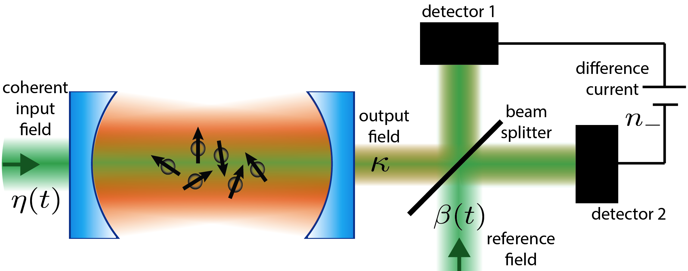
Figure 4: Illustration of a homodyne detection measurement which determines the response function $G^{R}(t,t^{\prime})$ of the cavity photons, see Ref. Buchhold et al. (2013). The system of atoms and photons inside the cavity is perturbed by the laser field $\eta(t)$, entering the cavity through the left mirror. The response of the system is encoded in the light field which is leaking out of the cavity on the right mirror with a rate $\kappa$. It can be measured by a standard homodyne detection measurement in which the reference laser $\beta(t)$ and a beam splitter are used in order to obtain information on the system’s coherence $\langle a_{c}(t)\rangle$. Figure copied from Ref. Buchhold et al. (2013). (Copyright (2013) by The American Physical Society.)

A closely related function of interest is the spectral function

$$A(\omega)=-2\mathop{\mathrm{Im}}G^{R}(\omega).$$ (61)

It is the distribution of excitation levels of the system, i.e., when adding a single photon with frequency $\omega$ to the system, $A(\omega)$ is the probability to hit the system at resonance. Indeed, it can be shown Altland and Simons (2010) that the spectral function is positive, $A(\omega)>0$, and fulfills the sum rule

$$\int_{\omega}A(\omega)=\langle[a,a^{\dagger}]\rangle=1.$$ (62)

For our example of a single-mode cavity, the spectral function is given by

$$A(\omega)=\frac{2\kappa}{\left(\omega-\omega_{0}\right)^{2}+\kappa^{2}},$$ (63)

i.e., it is a Lorentzian, which is centered at the cavity frequency $\omega_{0}$ and has a half-width at half-maximum given by $\kappa$. Note that for $\kappa\to 0$, the photon number states become exact eigenstates and the spectral density reduces to a $\delta$-function peaked at $\omega_{0}$, $A(\omega)=2\pi\delta(\omega-\omega_{0}).$ As these considerations illustrate, the retarded Green’s function contains essential information on the system’s response towards an external perturbation, and on the spectral properties.

Correlations: The Keldysh Green’s function contains elementary information on the system’s correlations and the occupation of the individual quantum mechanical modes. A prominent example of a correlation function in quantum optics is the photonic $g^{(2)}$ correlation function. It is defined as the four-point correlator

$$g^{(2)}(t,\tau)=\frac{\langle a^{\dagger}(t)a^{\dagger}(t+\tau)a(t+\tau)a(t)\rangle}{|\langle a^{\dagger}(t)a(t)\rangle|^{2}},$$ (64)

and it is proportional to the intensity fluctuations of the intracavity radiation field $g^{(2)}(t,\tau)\propto\langle I(t)I(t+\tau)\rangle$. In the limit of $\tau\rightarrow 0$, the $g^{(2)}$ correlation function reveals the statistics of the cavity photons, i.e., it demonstrates super-Poissonian ($g^{(2)}(0)>1$) or sub-Poissonian statistics ($g^{(2)}(0)<1$) as an effect of the light-matter interactions. In the absence of interactions (as in our example), it is straightforward to show that

$$g^{(2)}(t,\tau)=1+\frac{|G^{K}(t,\tau+t)+G^{R}(t,\tau+t)-G^{A}(t,\tau+t)|^{2}}{|iG^{K}(t,t)-1|^{2}}.$$ (65)

For equal times, the retarded and advanced Green’s functions satisfy $G^{R}(t,t)-G^{A}(t,t)=-i$, indicating the expected photon-bunching at $\tau\rightarrow 0$. On the other hand, in the presence of interactions, Eq. (64) is modified and contains additional higher order terms, as well as off-diagonal contributions. However, it remains a measure of the photonic statistics in the cavity due to the physical relation to the intensity fluctuations.

A particularly relevant and instructive limit of the two-time Keldysh Green’s function Eq. (52) concerns equal times $t=t^{\prime}$, which in general describes static correlation functions, or covariances in the quantum optics language. In the cavity example, it yields the mode occupation number,

$$iG^{K}(t,t)=2\langle a^{\dagger}a\rangle+1.$$ (66)

The appearance of the combination $2\langle a^{\dagger}a\rangle+1$ is rather intuitive when taking into account the relation to the operatorial formalism. Indeed, in operator language, $2a^{\dagger}a+1=\{a,a^{\dagger}\}=\{a^{\dagger},a\}$ is invariant under permutation of the operators $a,a^{\dagger}$, and therefore lends itself to a direct functional integral representation, which in fact carries no information on operator ordering. At the same time, the anticommutator carries all the physical information on state occupation, while the commutator carries none, $[a,a^{\dagger}]=1$ (note $a^{\dagger}a=\tfrac{1}{2}(\{a,a^{\dagger}\}-[a,a^{\dagger}])$).

Then, the explicit form of the Keldysh Green’s function stated in Eq. (47) leads to the result

$$\langle a^{\dagger}a\rangle=\frac{1}{2}\left(i\int_{\omega}G^{K}(\omega)-1\right)=0,$$ (67)

showing that the cavity is empty in the steady state—which is not surprising in the absence of external pumping.

We note that in the master equation formalism, information on the static or spatial correlations is most easily accessible — only the state (density matrix) has to be known, but not the dynamics acting on it. Temporal correlation functions can be extracted using the quantum regression theorem Walls and Milburn (2008). In the Keldysh formalism, spatial and temporal correlation functions are treated on an equal footing.

We can concisely summarize the above discussion of the response and Keldysh Green’s functions of the system, at the risk of oversimplifying:

Responses $G^{R/A}\leftrightarrow$ spectral information on excitations: which excitations are there?
Correlations $G^{K}\leftrightarrow$ statistical information on excitations: how are the excitations occupied?

Relation to thermodynamic equilibrium — Before we move on, let us briefly discuss how we have to modify the formalism in order to describe a cavity in thermodynamic equilibrium. In general, a system is in thermodynamic equilibrium at a temperature $T=1/\beta$, if it is in a Gibbs state $\rho=e^{-\beta H}/Z$ where $Z=\mathop{\mathrm{tr}}e^{-\beta H}$, and its dynamics is coherent and generated by the Hamiltonian $H$. (In particular, dissipative dynamics described by a term in the Lindblad form in Eq. (16) is not compatible with equilibrium conditions: see Refs. Talkner (1986); Ford and O’Connell (1996); Sieberer et al. (2015), and the discussion in Sec. II.4.1.) Specifying the thermal density matrix at $t_{0}$ in the Keldysh functional integral in Eq. (25) explicitly in terms of its matrix elements is rather inconvenient, especially if one is interested in steady state properties and wants to take the limit $t_{0}\to-\infty.$ An alternative is suggested by the observation that thermodynamic equilibrium can be established in the system if it is weakly coupled to a thermal bath. Then, the finite decay rate $\kappa$ in the retarded Green’s function in Eq. (46) should be replaced by an infinitesimally weak system-bath coupling $\delta\to 0$. Additionally, the Keldysh Green’s function has to be modified in such a way that the integral in Eq. (67) yields the Bose distribution function $n(\omega_{0})$ implying thermal occupations of the cavity mode,

$$\langle a^{\dagger}a\rangle=n(\omega_{0})=\frac{1}{e^{\beta\omega_{0}}-1}.$$ (68)

This can be achieved by replacing the Keldysh component of the inverse Green’s function in Eq. (43) by $P^{K}(\omega)=i2\delta\left(2n(\omega)+1\right)$. We emphasize the key structural difference of the thermal Keldysh component, which is strongly frequency dependent, to the Markovian case discussed previously, where this entry is frequency independent — this gives a strong hint that Markovian systems can behave quite differently from systems in thermal equilibrium. With $P^{R}(\omega)=P^{A}(\omega)^{*}=\omega-\omega_{0}-i\delta$ we obtain the equilibrium Green’s functions

$$G^{R}(\omega) =G^{A}(\omega)^{*}=\frac{1}{\omega-\omega_{0}+i\delta},$$ (69)

$$G^{K}(\omega) =-i2\pi\delta(\omega-\omega_{0})\left(2n(\omega)+1\right).$$ (70)

Note that the Green’s functions obey a thermal fluctuation-dissipation relation (FDR), which for the present example of a single bosonic mode reads

$$G^{K}(\omega)=\left(2n(\omega)+1\right)\left(G^{R}(\omega)-G^{A}(\omega)\right).$$ (71)

This is discussed in more detail in Sec. II.4.1. For the time being, let us mention that this construction to describe thermodynamic equilibrium by adding infinitesimal dissipative terms does not only work in the present case of a quadratic action but can also be applied in the interacting case. Then, the construction ensures that the free Green’s functions (i.e., the ones obtained by ignoring the interactions) obey an FDR. If the non-linear terms in the action obey the equilibrium symmetry discussed in Sec. II.4.1 (which is the case for generic interaction terms), this property is shared by the full Green’s functions of the non-linear system.

General Fluctuation-Dissipation Relations — While Eq. (71) is valid only in thermodynamic equilibrium, it is always possible to parameterize the (anti-Hermitian) Keldysh Green’s function in terms of the retarded and advanced Green’s functions (which, as discussed above, are Hermitian conjugates of each other) and a Hermitian matrix $F=F^{\dagger}$ in the form Kamenev (2011); Altland and Simons (2010)

$$G^{K}=G^{R}\circ F-F\circ G^{A},$$ (72)

where $\circ$ denotes convolution. In this parametrization, $F$ is the distribution function, which describes the distribution of (quasi-) particles over the modes of the system. For a non-equilibrium steady state, $F$ is time-translational invariant and its Fourier transform in frequency space $F(\omega)$ represents the energy resolved occupation of (quasi-) particle modes. On the other hand, as we discuss in detail in Sec. V.2, for the case of a time-evolving system, for which time translation invariance is absent, the Wigner transform of $F$ corresponds to the instantaneous local distribution function. For the important case of thermodynamic equilibrium (of a bosonic system), it is $F(\omega)=\coth(\beta\omega/2)=2n(\omega)+1$, and Eq. (72) reduces to (71). For the case where the bosonic Green’s function has a matrix structure in Nambu space, a subtlety concering the preservation of the symplectic structure of that space arises, cf. Sec. V.2. There, also a time-dependent variant of the non-equilibrium fluctuation-dissipation relations is discussed.

II.2.2 Driven-dissipative condensate

In the previous section, we discussed the simple case of a quadratic Keldysh action, which allowed us to perform the Keldysh functional integral explicitly. An additional simplification resulted from the fact that we were considering only a single bosonic mode. Let us now consider a genuine many-body problem, which is non-linear and in which the system consists of a continuum of modes. To be specific, in this section we discuss the model introduced in Sec. I.3.2 for a bosonic many-body system with interactions and non-linear loss processes (i.e., with a loss rate that is proportional to the density) in addition to the linear dissipative terms which were already present in the example of the single-mode cavity. Then, for a specific value of the mean-field density $\rho_{0}$, non-linear loss and linear pump exactly balance each other and the system reaches a stationary state. If $\rho_{0}$ is different from zero, this signals the presence of a condensate, which is accompanied by the breaking of a specific phase rotation symmetry as will be discussed in detail in Sec. II.4, and the establishment of long-range order. In Sec. IV, we give a detailed account of the influence of fluctuations on this driven-dissipative condensation transition. Here, we content ourselves with a mean-field analysis, which serves to illustrate some of the field theoretical concepts introduced in Sec. II.1 — in particular, the effective action and field equations — in a simple setting.

In the basis of classical and quantum fields, the Keldysh action associated with the quantum master equation (9) reads

$$S=\int_{t,\mathbf{x}}\left\{\phi_{q}^{*}\left(i\partial_{t}+K_{c}\nabla^{2}-r_{c}+ir_{d}\right)\phi_{c}+\mathrm{c.c.}\right.\\ -\left[\left(u_{c}-iu_{d}\right)\left(\phi_{q}^{*}\phi_{c}^{*}\phi_{c}^{2}+\phi_{q}^{*}\phi_{c}^{*}\phi_{q}^{2}\right)+\mathrm{c.c.}\right]\\ \left.+i2\left(\gamma+2u_{d}\phi_{c}^{*}\phi_{c}\right)\phi_{q}^{*}\phi_{q}\right\},$$ (73)

where $K_{c}=1/(2m_{\mathrm{LP}})$ and $r_{c}=\omega_{\mathrm{LP}}^{0}$; as additional parameters, we introduced the noise level $\gamma=(\gamma_{l}+\gamma_{p})/2$ and the spectral mass or gap $r_{d}=(\gamma_{l}-\gamma_{p})/2$. Hence, the rates of losses and pumping add up to the total noise level; in contrast, the difference of these rates enters in the spectral gap $r_{d}$, which becomes negative when the rate of incoherent pumping exceeds the single-particle loss rate, signaling the physical instability against condensation. In a mean-field analysis of the condensation transition, we perform a saddle-point approximation of the functional integral in Eq. (39). To leading order, fluctuations around the field expectation values are completely neglected. The expectation values are then obtained as spatially homogenous and stationary solutions to the classical field equations (here, “classical” refers to the fact that these field equations are derived from the classical (or: bare, microscopic) action $S$ discarding fluctuations, in contrast to the field equations in Eq. (40), which involve the effective action)

$$\frac{\delta S}{\delta\phi_{c}^{*}}=0,\quad\frac{\delta S}{\delta\phi_{q}^{*}}=0.$$ (74)

As already mentioned above in Sec. II.2.1, there are no terms in the action Eq. (38) with zero power of both $\phi_{q}^{*}$ and $\phi_{q}$, and the same is clearly true for $\delta S/\delta\phi_{c}^{*}$. Therefore, the first equation in (74) is solved by $\phi_{q}=0$. Inserting this condition into the second equation, we have

$$\left[-r_{c}+ir_{d}-\left(u_{c}-iu_{d}\right)\left\lvert\phi_{0}\right\rvert^{2}\right]\phi_{0}=0.$$ (75)

The solution $\phi_{c}=\phi_{0}$ is determined by the imaginary part of Eq. (75): for $r_{d}\geq 0$, in the so-called symmetric phase, the classical field expectation value is zero, $\rho_{0}=\left\lvert\phi_{0}\right\rvert^{2}=0$, whereas for $r_{d}<0$ we have a finite condensate density $\rho_{0}=-r_{d}/u_{d}$. Taking the real part of Eq. (75), we obtain for the parameter $r_{c}$ the relation $r_{c}=u_{c}r_{d}/u_{d}$. This condition can always be satisfied by proper choice of a rotating frame, i.e., by performing a gauge transformation $\phi_{c}\mapsto\phi_{c}e^{-i\omega t}$ such that $r_{c}\mapsto r_{c}-\omega$. In the original (laboratory) frame this simply means that the condensate amplitude oscillates at a finite frequency.

In a first step beyond mean field theory, quadratic fluctuations around the mean-field order parameter can be investigated within a Bogoliubov or tree-level expansion: we set $\phi_{c}=\phi_{0}+\delta\phi_{c},\phi_{q}=\delta\phi_{q}$ in the action Eq. (73) and expand the resulting expression to second order in the fluctuations $\delta\phi_{c,q}$. The inverse retarded, advanced and Keldysh Green’s functions now become $2\times 2$ matrices in the space of Nambu spinors $\delta\Phi_{\nu}=\left(\delta\phi_{\nu},\delta\phi_{\nu}^{*}\right)$. In particular, we have in the frequency and momentum domain

$$\begin{split}P^{R}(\omega,\mathbf{q})&=\begin{pmatrix}\omega-K_{c}q^{2}-\left(u_{c}-iu_{d}\right)\rho_{0}&-\left(u_{c}-iu_{d}\right)\rho_{0}\\ -\left(u_{c}+iu_{d}\right)\rho_{0}&-\omega-K_{c}q^{2}-\left(u_{c}+iu_{d}\right)\end{pmatrix},\\ P^{A}(\omega,\mathbf{q}))&=P^{R}(\omega,\mathbf{q})^{\dagger},\\ P^{K}&=i\gamma\mathbbm{1}.\end{split}$$ (76)

The excitation spectrum is obtained from the condition $\det P^{R}(\omega,\mathbf{q})=0$. Indeed, this is the condition for the field equation of the fluctuations $P^{R}(\omega,\mathbf{q})\delta\Phi_{c}(\omega,\mathbf{q})=0$ to have nontrivial solutions. This yields Wouters and Carusotto (2007a)

$$\omega_{1,2}^{R}=-iu_{d}\rho_{0}\pm\sqrt{K_{c}q^{2}\left(K_{c}q^{2}+2u_{c}\rho_{0}\right)-\left(u_{d}\rho_{0}\right)^{2}}.$$ (77)

We note that due to the tree-level shifts $\propto\rho_{0}$ the above described instability for $r_{d}<0$ is lifted: both poles are consistently located in the lower complex half-plane, indicating a physically stable situation with decaying single-particle excitations. For $u_{d}=0$, Eq. (77) reduces to the standard Bogoliubov result Lifshitz and Pitaevskii (1980), where for $q\to 0$ the dispersion is phononic, $\omega_{1,2}^{R}=\pm cq$ ($c=\sqrt{2K_{c}u_{c}\rho_{0}}$ the speed of sound), whereas particle-like behavior $\omega_{1,2}^{R}\sim K_{c}q^{2}$ is obtained at high momenta. Here, due to the presence of two-body loss $u_{d}\neq 0$, the dispersion is qualitatively modified: while at high momenta the dominant behavior is still $\omega_{1,2}^{R}\sim K_{c}q^{2}$, at low momenta we find purely incoherent diffusive, non-propagating modes $\omega_{1}^{R}\sim-i\frac{K_{c}u_{c}}{u_{d}}q^{2}$ and $\omega_{2}^{R}\sim-i2u_{d}\rho_{0}$. In particular, for $q=0$ we have $\omega_{1}^{R}=0$: this is a dissipative Goldstone mode Wouters and Carusotto (2006, 2007a); Szymańska et al. (2006), associated with the spontaneous breaking of the global $U(1)$ symmetry in the ordered phase. The existence of such a mode is not bound to the mean-field approximation, but rather is an exact property guaranteed by the $U(1)$ invariance of the effective action, even in the present case of a driven-dissipative condensate. We will come back to this point in Sec. II.4.6.

II.3 Semiclassical limit of the Keldysh action

The theoretical description of a many-body system depends crucially on the scale (this could be a length, time, or energy scale — in practice these scales can be expressed in terms of each other) on which it is observed and, in particular, on the relation between this observation scale and the intrinsic scales of the system. For example, at finite temperature $T$ above a quantum critical point, non-trivial quantum critical behavior can be observed at moderate energy scales which are larger than $T$ but smaller than the Ginzburg scale where fluctuations start to dominate over the mean field effects Sachdev (2011). On the other hand, classical thermal critical behavior, which is perfectly described by taking the semiclassical limit of the underlying quantum theory, sets in at energy scales below $T$. Out of thermodynamic equilibrium, the analogue of a finite temperature is Markovian noise. In the Keldysh action, this corresponds to a constant term in the Keldysh sector of the inverse Green’s function, i.e., a constant noise vertex. Such a term is present in the action given in Eq. (73) and, therefore, we expect that in the long-wavelength limit this action can actually be simplified by taking the semiclassical limit Kamenev (2011); Altland and Simons (2010). We refer to it as the semiclassical limit, as, e.g., effects of quantum mechanical phase coherence are not necessarily suppressed in this limit, as we will see. A useful equilibrium analogy is the physics of Bose-Einstein condensates at finite but low temperatures, where phase coherence still persists.

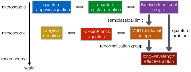
Figure 5: Equivalent descriptions on varying length scales. The quantum and classical Langevin equations are stochastic equations of motions for the field operators, or for classical field variables. In contrast, the descriptions in the middle column are deterministic equations of motion, where either a density operator or a probability distribution (diagonals of a density matrix) are evolved. In the functional integral formulation, the basic object in both quantum and classical cases is an action, which is averaged over all possible realizations of field configurations. The semiclassical limit is valid at mesoscopic scales as dicsussed in Sec. II.3. An effective description at macroscopic scales can be obtained by means of renormalization group methods (see Sec. II.5). Generically in Markovian systems, in order to reduce the complexity of the problem it is useful to first perform the semiclassical limit before doing a renormalization group computation. However, in driven open quantum systems there are also circumstances where this is inappropriate, and the full quantum problem has to be analyzed, cf. Marino and Diehl (2016).

Formally, the suitability of the semiclassical limit can be understood in terms of ideas that lie at the basis of the renormalization group (RG). The latter provides a recipe for finding an effective description that is valid on large length scales, starting from a microscopic theory. Various RG schemes exist, which allow to systematically eliminate fluctuations on short scales and infer their influence on the effective description of the system on large scales; cf. Sec. II.5. The most basic but still informative RG approach however consists in simply ignoring the effect of short-scale fluctuations: one subdivides momentum space into a slow and a fast region, with $q_{s}\in[0,\Lambda/b]$ and $q_{f}\in[\Lambda/b,\Lambda]$ where $\Lambda$ is the UV cutoff (given by the inverse of some microscopic length scale below which the theoretical description is not valid any more, e.g., a lattice spacing) and $b>1$, and omits all contributions to the action which involve fluctuations with fast momenta. In a second step, one rescales all momenta with $b$ to restore the original range of momenta $q\in[0,\Lambda]$, and the thus obtained effective long-wavelength description can be compared to the original one. As a result, due to this simple RG transformation couplings in the action are rescaled as $g\mapsto gb^{d_{g}}$, where $d_{g}$ is known as the canonical scaling dimension of $g$. Evidently, for $d_{g}>0$, $g$ grows under renormalization and hence $g$ is a relevant coupling, while it shrinks under renormalization and, hence, is irrelevant at long wavelength for $d_{g}<0$. For the case of a marginal coupling with $d_{g}=0$, this level of approximation is not conclusive as to whether the coupling becomes larger or smaller under renormalization. Classifying the coupling parameters of an action according to this scheme is known as canonical scaling analysis, or power counting. A useful approximation consists in neglecting all irrelevant couplings. On the other hand, relevant couplings which are compatible with the symmetries of the model – even those, which are not present in the microscopic description — should be included in the long-wavelength effective action.

Let us perform such an analysis for the Keldysh action in Eq. (73). We can anticipate the canonical scaling dimensions by noting that they are just the physical dimensions, measured in powers of the momentum. We first focus on the vicinity of the threshold for condensation, i.e., when $r_{d}\sim\gamma_{l}-\gamma_{p}\to 0$. Then the retarded and advanced inverse Green’s functions scale as $P^{R/A}\sim q^{2}$ (note that $\omega\sim q^{2}$ for low-momentum excitations). The canonical dimension is thus positive, $d_{P^{R/A}}=2$. On the other hand, as anticipated above, Markovian noise analogous to a finite temperature corresponds to a momentum-independent noise vertex, i.e., the term $\propto\phi_{q}^{*}\phi_{q}$ in the Keldysh action. In other words, the Keldysh component of the inverse Green’s function has vanishing canonical scaling dimension and classifies as marginal, $P^{K}=i2\gamma\sim q^{0}$. We furthermore use the natural scaling $d^{d}\mathbf{x}\sim q^{-d}$ and $dt\sim 1/\omega\sim q^{-2}$, and the condition of scale invariance of the action, $S\sim q^{0}$ — this is a requirement stemming from the fact that the action appears in the exponent of the functional integral (25), and thus must be dimensionless. We then find the scaling dimensions of the fields from the Gaussian, quadratic part of the action to be

$$\phi_{c}\sim q^{(d-2)/2},\quad\phi_{q}\sim q^{(d+2)/2}.$$ (78)

This in turn allows us to derive the scaling dimensions of the quartic terms, and to classify their degree of relevance as pointed out above. In particular, we find that in three spatial dimensions, any quartic term that includes more than a single quantum field is irrelevant; the only non-irrelevant term of higher order in the noise field is the quadratic noise vertex discussed above. Therefore, omitting irrelevant terms amounts to keeping only the classical vertex in the action Eq. (73), i.e., to taking the semiclassical limit Kamenev (2011); Altland and Simons (2010). Then, the Keldysh action takes the form

$$S=\int_{t,\mathbf{x}}\left\{\phi_{q}^{*}\left[i\partial_{t}+\left(K_{c}-iK_{d}\right)\nabla^{2}-r_{c}+ir_{d}\right]\phi_{c}+\mathrm{c.c.}\right.\\ \left.-\left[\left(u_{c}-iu_{d}\right)\phi_{q}^{*}\phi_{c}^{*}\phi_{c}^{2}+\mathrm{c.c.}\right]+i2\gamma\phi_{q}^{*}\phi_{q}\right\},$$ (79)

where in addition to omitting irrelevant contributions we have added an effective diffusion term $\propto iK_{d}\nabla^{2}$. Such a term can and will be generated upon integrating out short-scale fluctuations Sieberer et al. (2013, 2014). Moreover, a complex prefactor of the term involving the derivative with respect to time, which also emerges upon renormalization, can be absorbed into a redefinition of the fields.

Strictly speaking, the above analysis is valid in the vicinity of the critical point only, where the inverse retarded and advanced Green’s function show scaling. However, as long as one is close enough to threshold $\lvert\gamma_{l}-\gamma_{p}\rvert/(\gamma_{l}+\gamma_{p})\ll 1$, the canonical power counting is expected to give a useful orientation in the problem.

Apart from providing a significant simplification, taking the semiclassical limit also allows us to establish the connection Zhou et al. (1980); Chou et al. (1985) between the Keldysh functional integral formalism and the more traditional formulation of dynamics close to a continuous phase transition in terms of Langevin equations Hohenberg and Halperin (1977); Täuber (2014). In fact, the action in Eq. (79) is fully equivalent to the following Langevin equation:

$$i\partial_{t}\phi_{c}=\left[-\left(K_{c}-iK_{d}\right)\nabla^{2}+r_{c}-ir_{d}+\left(u_{c}-iu_{d}\right)\left\lvert\phi_{c}\right\rvert^{2}\right]\phi_{c}+\xi,$$ (80)

where $\xi$ is a Markovian Gaussian noise source with zero mean, $\langle\xi(t,\mathbf{x})\rangle=0,$ and second moment $\langle\xi(t,\mathbf{x})\xi(t^{\prime},\mathbf{x}^{\prime})\rangle=2\gamma\delta(t-t^{\prime})\delta(\mathbf{x}-\mathbf{x}^{\prime})$. This equivalence can be established by means of a Hubbard-Stratonovich transformation of the noise vertex Kamenev (2011); Altland and Simons (2010), i.e., the term $i2\gamma\phi_{q}^{*}\phi_{q}$. To wit, in the Keldysh functional integral

$$Z=\int\mathscr{D}[\phi_{c},\phi_{c}^{*},\phi_{q},\phi_{q}^{*}]\,e^{iS[\phi_{c},\phi_{c}^{*},\phi_{q},\phi_{q}^{*}]},$$ (81)

where $S$ is the semiclassical action in Eq. (79), we write the noise vertex as a Gaussian integral over an auxiliary variable $\xi$ (cf. Appendix B),

$$e^{-2\gamma\int_{t,\mathbf{x}}\phi_{q}^{*}\phi_{q}}=\int\mathscr{D}[\xi,\xi^{*}]\,e^{-\frac{1}{2\gamma}\int_{t,\mathbf{x}}\xi^{*}\xi-i\int_{t,\mathbf{x}}\left(\phi_{q}^{*}\xi-\xi^{*}\phi_{q}\right)}.$$ (82)

As a result, the exponent in the functional integral (81) becomes linear in the quantum field, and the corresponding integration can be performed, resulting in a $\delta$-functional,

$$Z=\int\mathscr{D}[\phi_{c},\phi_{c}^{*},\xi,\xi^{*}]\,e^{-\frac{1}{2\gamma}\int_{t,\mathbf{x}}\xi^{*}\xi}\\ \times\delta\!\left(\left[i\partial_{t}+\left(K_{c}-iK_{d}\right)\nabla^{2}-r_{c}+ir_{d}-\left(u_{c}-iu_{d}\right)\left\lvert\phi_{c}\right\rvert^{2}\right]\phi_{c}-\xi\right)\\ \times\delta\!\left(\left[-i\partial_{t}+\left(K_{c}+iK_{d}\right)\nabla^{2}-r_{c}-ir_{d}-\left(u_{c}+iu_{d}\right)\left\lvert\phi_{c}\right\rvert^{2}\right]\phi_{c}^{*}-\xi^{*}\right).$$ (83)

This expression can be interpreted as follows: for a given realization of the noise field $\xi$, the $\delta$-functional restricts the functional integral over $\phi_{c}$ to the manifold of solutions to the Langevin equation (80). The statistics of the noise field is determined by the Gaussian weight factor in Eq. (83). Correlation functions of classical fields can then be calculated by picking a random realization of $\xi$ and calculating the corresponding $\phi_{c}$ that solves the Langevin equation; evaluating the correlation function for this solution and finally averaging the result according to the Gaussian distribution of the noise field. Equation (80) is, therefore, equivalent to the functional integral (83) in that it allows for the evaluation of arbitrary correlation functions.

Originally, Langevin equations like Eq. (80) have been introduced as a phenomenological description of the coarse-grained dynamics of the order parameter, and only later a functional integral approach — known as the MSR approach — has been developed Martin et al. (1973); De Dominicis (1976); Janssen (1976); Bausch et al. (1976). The action derived in these references is formally equivalent to the one in Eq. (79), with $\phi_{c}$ taking the role of the order parameter field, while the field that corresponds to $\phi_{q}$ is known as the response field.

In addition to the descriptions of semiclassical dynamical models in terms of a semiclassical Keldysh (or MSR) functional integral or a Langevin equation, there exists yet another equivalent approach, in which the stochastic Langevin equation for the classical field or order parameter field is replaced by a deterministic evolution equation for the probability distribution of the latter, known as the Fokker-Planck equation. The derivation of the Fokker-Planck equation can be found, e.g., in Refs. Altland and Simons (2010); Kamenev (2011); Täuber (2014); Chaikin and Lubensky (1995). Figure 5 illustrates the equivalence of these approaches, which are valid on a (coarse-grained) mesoscopic scale, and the relations to microscopic and macroscopic descriptions.

II.4 Symmetries of the Keldysh action

Symmetries take center stage in field theories. Translating the physics of the quantum master equation to the Keldysh functional integral allows us to leverage the power of symmetry considerations over to the context of open systems. In this section, we discuss three different aspects of symmetries.

The presence of a first, discrete symmetry, considered in Sec. II.4.1, allows us to conclude whether or not a quantum or classical system is situated in the realm of thermodynamic equilibrium. This symmetry is equivalent to the validity of thermal fluctuation-dissipation relations (cf. Sec. II.2.1) for correlation functions of any order and can be connected to energy conservation. Thermal equilibrium can thus be diagnosed by means a of simple symmetry test on the Keldysh action. In particular, we argue that Markovian quantum master equations explicitly violate this symmetry, indicating non-equilibrium conditions. In the semiclassical limit, we obtain a simple and intuitive geometric interpretation of the symmetry and its absence under non-equilibrium drive in terms of the location of the coupling constants of the effective action in the complex plane.

A second fundamental consequence of the presence of symmetries — now, continous global symmetries — is the Noether theorem, stating that such symmetries imply conserved charges. In Sec. II.4.3, we discuss the Noether theorem in the context of the Keldysh formalism. Working on the Keldysh contour, we have to distinguish between two symmetry transformations, for each the forward and backward branches of the closed time path. In the basis of classical and quantum fields, we can identify “classical” symmetry transformations, which act in the same way on fields on the forward and backward branches, and “quantum” transformations, for which the transformation of the fields on the backward branch is the inverse of the transformation on the forward branch. Non-trivial conservation laws follow only from the symmetry of the Keldysh action under quantum transformations. We illustrate this point with the example of the symmetry of the action of a closed system with respect to space-time translations and phase rotations in Sec. II.4.4, which entails conservation of energy and momentum and the number of particles, respectively. On the other hand, in open systems, in which the number of particles is not conserved, only classical phase rotations are a symmetry of the action, and the continuity equation that is implied by particle number conservation has to be extended as detailed in Sec. II.4.5.

Finally, another consequence of a global continuous symmetry is the existence of gapless modes in case that this symmetry is broken spontaneously, as in a Bose condensation transition. In a driven-dissipative condensate in which the number of particles is not conserved (cf. Sec. II.2.2), we show that the symmetry which is broken spontaneously at the condensation transition is the classical phase rotation symmetry, and we work out the Goldstone theorem, which guarantees the existence of a massless mode, for this case in Sec. II.4.6.

II.4.1 Thermodynamic equilibrium as a symmetry of the Keldysh action

A system is in thermodynamic equilibrium at a temperature $T=1/\beta$, if (i) the density matrix is given by $\rho=e^{-\beta H}/Z$ where $Z=\mathop{\mathrm{tr}}e^{-\beta H}$, and (ii) the very same Hamiltonian operator $H$ appearing in $\rho$ generates the unitary time evolution of the system, $U=e^{-iHt}$. Condition (ii) implies that static correlations are in general not sufficient to prove that a system is in thermal equilibrium; however, dynamical correlations are: this can be inferred from the fact that the static correlations of a physical system can always be encoded in a density matrix $\rho$, and the latter can always be parameterized formally as an equilibrium density matrix, $\rho=e^{-\beta H^{\prime}}/Z^{\prime}$, with a Hermitian operator $H^{\prime}$. (In other words, any state can be thought of as a thermal state with respect to some Hamiltonian.) On the other hand, static (i.e., purely momentum- or space-dependent) properties do not allow us to discriminate whether the generator of dynamics coincides with $H^{\prime}$. In sharp contrast, any dynamical (i.e., frequency- or time-dependent) observable is manifestly governed by this generator, as is easily seen in the Heisenberg picture (or a suitable generalization to open systems). Response functions at finite frequency are such dynamical observables, and the equilibrium conditions formulated above are reflected in the fact that in thermodynamic equilibrium the response of the system to an external perturbation at a frequency $\omega$ is related to thermal fluctuations within the system at the same frequency by what is known as a fluctuation-dissipation relation Kubo (1966) (FDR; for a discussion in the context of non-equilibrium Bose-Einstein condensation see Ref. Chiocchetta et al. (2015a)). Such a relation, which is equivalent to the combination of the Kubo-Martin-Schwinger (KMS) condition Kubo (1957); Martin and Schwinger (1959) with time reversal Jakobs et al. (2010a), is valid for any pair of operators. In particular, for the case that these are the basic field operators of a single-component Bose system at the temperature $T=1/\beta$, the FDR reads (note that this is a generalization of Eq. (71) to the case of a spatial continuum of degrees of freedom)

$$G^{K}(\omega,\mathbf{q})=\coth\!\left(\frac{\omega}{2T}\right)(G^{R}(\omega,\mathbf{q})-G^{A}(\omega,\mathbf{q}))$$ (84)

(in the presence of a chemical potential $\mu$, in the argument of the trigonometric function we have to shift $\omega\to\omega-\mu$). In quantum field theory, relations among Green’s functions often follow as consequences of a symmetry of the action. Then, they are known as Ward-Takahashi identities associated with the symmetry Zinn-Justin (2002); Peskin and Schroeder (1995). This raises the question, whether FDRs and hence the presence of thermodynamic equilibrium conditions are also connected to a symmetry of the Keldysh action.

To make the point clear, let us rephrase the question: above we made the observation, that the defining property of (canonical) thermal equilibrium is the validity of FDRs. Importantly, these FDRs hold for correlation functions of arbitrary order, i.e., not just the two-point Keldysh Green’s function in Eq. (84) can be expressed through response functions, but also any higher order correlation function is determined by corresponding higher order response functions. Then, the question — which we answer in the affirmative below — is, whether this infinite hierarchy of FDRs expressing thermal equilibrium is related to a structural property of the theory. Indeed, this structural property is a symmetry of the Keldysh action, i.e., a transformation of the fields $\Psi\mapsto\mathcal{T}_{\beta}\Psi$ such that

$$S[\Psi]=\tilde{S}[\mathcal{T}_{\beta}\Psi].$$ (85)

Here, we denote $\Psi=\left(\psi_{+},\psi_{+}^{*},\psi_{-},\psi_{-}^{*}\right)$, and we specify the precise form of $\mathcal{T}_{\beta}$ below in Eq. (88). The tilde on the RHS of the equation indicates that all external fields appearing, $S$ have to be replaced by their corresponding time-reversed values. To name an example, the signs of magnetic fields have to be inverted Sieberer et al. (2015). Evidently, discussing a single symmetry instead of an infinite hierarchy of equations is much more elegant and practical: checking whether a given Keldysh action obeys Eq. (85) is straightforward and can be accomplished in finite time, in contrast to verifying the full set of FDRs.

It is easily seen, how these FDRs can be deduced as a consequence of the symmetry of the Keldysh action (85). To this end, we note by a Keldysh rotation (32) and after Fourier transformation, the Green’s functions appearing in Eq. (84) can be expressed as a sum of averages of the form $\langle\psi_{\sigma}(t,\mathbf{x})\psi_{\sigma^{\prime}}^{*}(t^{\prime},\mathbf{x}^{\prime})\rangle$. Writing these explicitly as field integrals, and anticipating that a change of integration variables $\Psi\to\mathcal{T}_{\beta}\Psi$ leaves the functional measure $\mathscr{D}[\Psi]$ invariant Sieberer et al. (2015), we find

$$\begin{split}\langle\psi_{\sigma}(t,\mathbf{x})\psi_{\sigma^{\prime}}^{*}(t^{\prime},\mathbf{x}^{\prime})\rangle&=\int\mathscr{D}[\Psi]\,\psi_{\sigma}(t,\mathbf{x})\psi_{\sigma^{\prime}}^{*}(t^{\prime},\mathbf{x}^{\prime})e^{iS[\Psi]}\\ &=\int\mathscr{D}[\mathcal{T}_{\beta}\Psi]\,\mathcal{T}_{\beta}\psi_{\sigma}(t,\mathbf{x})\mathcal{T}_{\beta}\psi_{\sigma^{\prime}}^{*}(t^{\prime},\mathbf{x}^{\prime})e^{iS[\mathcal{T}_{\beta}\Psi]}\\ &=\langle\mathcal{T}_{\beta}\psi_{\sigma}(t,\mathbf{x})\mathcal{T}_{\beta}\psi_{\sigma^{\prime}}^{*}(t^{\prime},\mathbf{x}^{\prime})\rangle.\end{split}$$ (86)

In the last equality, we used the symmetry of the Keldysh action (85) (assuming for simplicity that there are no external fields). Inserting here the explicit form of the symmetry transformation specified in Eq. (88) below where $\beta=1/T$ is the inverse temperature, it can be seen that Eq. (86) is in fact equivalent to the FDR (84) Sieberer et al. (2015).

By generalizing this argument to arbitrary field averages, one can establish the full equivalence between the infinite hierarchy of FDRs and the symmetry property of the Keldysh action (85) Sieberer et al. (2015). Thus, the symmetry of the Keldysh action under this transformation is a direct proof of the presence of thermodynamic equilibrium conditions. The existence of a symmetry that is related to thermal equilibrium has first been realized in the context of classical stochastic models Janssen (1976); Bausch et al. (1976); Janssen (1979); Aron et al. (2010, 2014), and these considerations have been extended to the realm of quantum systems in Refs. Altland et al. (2010); Sieberer et al. (2015).

What is the explicit form of the transformation $\mathcal{T}_{\beta}$? We can guess its essential ingredients by reminding ourselves that, as stated above Eq. (84), FDRs can be obtained from the KMS condition Kubo (1957); Martin and Schwinger (1959). The latter reads, for operators $A(t)=e^{iHt}A(0)e^{-iHt}$ and $B(t^{\prime})$ in the Heisenberg representation,

$$\langle A(t)B(t^{\prime})\rangle=\langle B(t^{\prime})A(t+i\beta)\rangle.$$ (87)

Comparing this with Eq. (86) indicates that $\mathcal{T}_{\beta}$ involves a translation of $t$ into the complex plane by an amount proportional to the inverse temperature $\beta$. Moreover, the order of operators on the RHS of the KMS condition is reversed as compared to the LHS. The original time order can be restored by means of a time reversal transformation Messiah (1965) — this step is necessary in order to obtain a time-ordered expression which can be expressed as a Keldysh field integral (by construction, field integrals yield time-ordered averages Negele and Orland (1998)). A careful analysis Sieberer et al. (2015) leads to the precise form of the thermal symmetry transformation ($\sigma=+(-)$ for fields on the forward (backward) branch):

$$\begin{split}\mathcal{T}_{\beta}\psi_{\sigma}(t,\mathbf{x})&=\psi_{\sigma}^{*}(-t+i\sigma\beta/2,\mathbf{x}),\\ \mathcal{T}_{\beta}\psi_{\sigma}^{*}(t,\mathbf{x})&=\psi_{\sigma}(-t+i\sigma\beta/2,\mathbf{x})\end{split}$$ (88)

(in the presence of a chemical potential $\mu$, we have to multiply the RHS of the first (second) line by $e^{\sigma\beta\mu/2}(e^{-\sigma\beta\mu/2})$). The transformation $\mathcal{T}_{\beta}$ is a composition of complex conjugation of the fields $\psi_{\sigma}$ and inversion of the sign of the time $t$ — both originating from the time reversal transformation —, and translation of the value of $t$ by an amount $i\sigma\beta/2$. The latter is induced by the KMS condition Eq. (87). We note that the translation of $t$ in Eq. (88) takes opposite signs depending on whether a field on the forward or on the backward branch is being transformed. As we show in Sec. II.4.4 below, a similar form of time translations is connected to conservation of energy: indeed, if the Keldysh action is invariant under time translations $\psi_{\sigma}(t,\mathbf{x})\mapsto\psi_{\sigma}(t+\sigma s,\mathbf{x})$ with $s\in\mathbb{R}$, the total energy in the system is conserved. A crucial difference from the time translation that is part of $\mathcal{T}_{\beta}$ is that energy conservation requires invariance under shifts by an arbitrary real value $s$, whereas $\mathcal{T}_{\beta}$ involves a shift by the purely imaginary value $i\beta/2,$ where $\beta=1/T$ is fixed and determined by the temperature.

Under which conditions does the Keldysh action (30) with $\mathcal{L}$ defined in Eq. (28) have the thermal symmetry, i.e., under which conditions does it describe a system in thermal equilibrium? Let us first consider the parts of the action corresponding to unitary time evolution, i.e., the first two terms in Eq. (30) and the first line in Eq. (28). It is straightforward to check Sieberer et al. (2015) that these terms are symmetric if the Hamiltonian densities $H_{\pm}$ do not explicitly depend on time. On the other hand, adding an external classical driving field such as a laser, and thus breaking time translational invariance by making $H_{\pm}$ time dependent, also the thermal symmetry is broken . The violation of the thermal symmetry by classical driving fields on the level of a microscopic Hamiltonian description indicates that quantum master equations correspond to genuine non-equilibrium conditions Sieberer et al. (2015); Talkner (1986); Ford and O’Connell (1996). Physically, this is due to the fact that a system for which such a description is appropriate is necessarily driven.

In an effective description of a driven-dissipative system in terms of a Markovian master equation in a rotating frame, there is often no explicit time dependence — indeed, our derivation of the dissipative Keldysh action in Sec. II.1 started from Eq. (16) with time-independent Hamiltonian. Even then, the thermal symmetry can be used to diagnose non-equilibrium conditions Sieberer et al. (2015). Again, it is sufficient to study only the time-translation part of $\mathcal{T}_{\beta}$: for time-independent $H_{\pm}$ and $L_{\alpha,\pm}$ in Eq. (28), the Keldysh action is still invariant under time translations of the form $\psi_{\sigma}(t,\mathbf{x})\mapsto\psi_{\sigma}(t+s,\mathbf{x})$. Importantly, this differs from the time translation that occurs in $\mathcal{T}_{\beta}$ by the absence of a factor of $\sigma$, meaning that $t$ is shifted by the same amount on the forward and backward branches. Then, by means of a simple shift of the integration variable $t$ in Eq. (30) the original form of the action can be restored. This strategy fails for the dissipative contributions in Eq. (28) that couple forward and backward branches, when the transformation involves the contour index $\sigma$. Again we reach the conclusion that quantum master equations describe genuine non-equilibrium conditions, even though by a slightly different argument than in the driven but purely Hamiltonian setting.

In some cases, the Markov and rotating-wave approximations leading to a description in terms of a quantum master equation or equivalent Keldysh action are applied in the absence of external driving fields. Then, these approximations might still be justified to study the behavior of specific observables, even though they explicitly break the symmetry Sieberer et al. (2015). To give an example, if one attempts to study thermalization of a system due to the coupling with a heat bath, and one integrates out the bath using the above-mentioned approximations, the resulting dynamics of the system will still lead to a thermal stationary state. Correspondingly, all static properties of the system will appear thermal. However, as discussed at the beginning of the present section, to unambiguously prove the presence of thermal equilibrium conditions, one has to consider dynamical signatures such as FDRs. Then, as a consequence of the explicit violation of the thermal symmetry by the Markov and rotating-wave approximations, the description of the system dynamics in terms of a quantum master equation will lead to the wrong prediction that fluctuations in the system do not obey an FDR.

A simple example that illustrates the above discussion is given by a single bosonic mode $a$ with energy $\omega_{0}$, driven coherently at a frequency $\omega_{l}$, and coupled to a bath of harmonic oscillators $b_{\mu}$ in thermal equilibrium. The associated Keldysh action can be decomposed as $S=S_{s}+S_{sb}+S_{b}$, where the action for the system consists of two parts, $S_{s}=S_{0}+S_{l}$ which read

$$S_{0}=\sum_{\sigma}\sigma\int_{\omega}a_{\sigma}^{*}(\omega)\left(\omega-\omega_{0}\right)a_{\sigma}(\omega),$$ (89)

and

$$\begin{split}S_{l}&=\Omega\sum_{\sigma}\sigma\int dt\left(a_{\sigma}(t)e^{i\omega_{l}t}+a_{\sigma}^{*}(t)e^{-i\omega_{l}t}\right)\\ &=\Omega\sum_{\sigma}\sigma\left(a_{\sigma}(\omega_{l})+a_{\sigma}^{*}(\omega_{l})\right).\end{split}$$ (90)

$\Omega$ is the amplitude of the driving field, and due to the harmonic time dependence of the drive it affects only the component $a(\omega_{l})$ in frequency space. The action for the bath is expressed most conveniently in the basis of classical and quantum fields (cf. Eq. (32)). In addition to the coherent part stemming from the oscillator frequencies, it involves infinitesimal dissipative regularization terms specifying the thermal equilibrium state of the bath at inverse temperature $\beta=1/T$ as discussed in Sec. II.2.1,

$$S_{b}=\sum_{\mu}\int_{\omega}\begin{pmatrix}b_{\mu,c}^{*}(\omega),b_{\mu,q}^{*}(\omega)\end{pmatrix}\\ \times\begin{pmatrix}0&\omega-\omega_{\mu}-i\delta\\ \omega-\omega_{\mu}+i\delta&i2\delta\coth(\beta\omega/2)\end{pmatrix}\begin{pmatrix}b_{\mu,c}(\omega)\\ b_{\mu,q}(\omega)\end{pmatrix}.$$ (91)

Finally, the system-bath interaction with coupling strength $\lambda$ corresponds to the following contribution to the action:

$$S_{sb}=\lambda\sum_{\sigma}\sigma\sum_{\mu}\int_{\omega}\left(a_{\sigma}^{*}(\omega)b_{\mu,\sigma}(\omega)+a_{\sigma}(\omega)b_{\mu,\sigma}^{*}(\omega)\right).$$ (92)

To check whether the transformation (88) is a symmetry of the action even in the presence of the driving term in Eq. (90), it is most convenient to rewrite the transformation in frequency space. Moreover, for future reference, we give the form of the transformation including a chemical potential:

$$\begin{split}\mathcal{T}_{\beta,\mu}a_{\sigma}(\omega)&=e^{-\sigma\beta\left(\omega-\mu\right)/2}a_{\sigma}^{*}(\omega),\\ \mathcal{T}_{\beta,\mu}a_{\sigma}^{*}(\omega)&=e^{\sigma\beta\left(\omega-\mu\right)/2}a_{\sigma}(\omega).\end{split}$$ (93)

It is straightforward to check that both $S_{b}$ and $S_{sb}$ are invariant under this transformation with $\mu=0$ Sieberer et al. (2015); the same holds true for the contribution $S_{0}$ to the action of the system. However, the driving part (90) becomes after the transformation

$$S_{l}=\Omega\sum_{\sigma}\sigma\left(a_{\sigma}(\omega_{l})e^{\sigma\beta\omega_{l}/2}+a_{\sigma}^{*}(\omega_{l})e^{-\sigma\beta\omega_{l}/2}\right),$$ (94)

where the appearance of the exponentials shows that the symmetry is violated. One might wonder whether it is possible to restore the symmetry in a rotating frame in which the explicit time dependence of the action is eliminated, i.e., by introducing new variables $\tilde{a}_{\sigma}(t)$ and $\tilde{b}_{\sigma}(t)$ rotating at the frequency of the driving field, $\tilde{a}_{\sigma}(t)=a_{\sigma}(t)e^{i\omega_{l}t}$ and analogously for $\tilde{b}_{\sigma}(t)$. In terms of these variables, the driving part of the action becomes

$$\begin{split}S_{l}&=\Omega\sum_{\sigma}\sigma\int dt\left(\tilde{a}_{\sigma}(t)+\tilde{a}_{\sigma}^{*}(t)\right)\\ &=\Omega\sum_{\sigma}\sigma\left(\tilde{a}_{\sigma}(0)+\tilde{a}_{\sigma}^{*}(0)\right),\end{split}$$ (95)

i.e., the drive couples to the zero-frequency component of $\tilde{a}_{\sigma}(\omega)$. Clearly, applying again the same transformation Eq. (93) with $\mu=0$ to the new variables, the driving term, as well as $S_{0}$ in Eq. (89) and the system-bath coupling $S_{sb}$ in Eq. (92) are invariant. However, in the action for the bath (91), as a consequence of the transformation to the rotating frame the distribution function acquires an effective chemical potential and becomes $\coth(\beta(\omega-\omega_{l})/2)$. Hence, to leave this part of the action invariant, the transformation Eq. (93) has to be applied with $\mu=\omega_{l}$, and again the full action is not invariant under the equilibrium transformation. No frame exists in which the reference to the driving scale $\omega_{l}$ were eliminated.

While this simple example demonstrates explicitly that generically external driving takes a system out of thermal equilibrium, and how this is manifest in the symmetry properties of the Keldysh action, it is interesting to note that there are surprising exceptions to this rule, emerging as limiting cases. One of them has been identified in Ref. Hafezi et al. (2014). Along the lines of this reference, we discard the driving term $S_{l}$ and instead consider a parametric system-bath coupling of the form

$$\begin{split}S_{sb}&=\lambda\sum_{\sigma}\sigma\sum_{\mu}\int dt\left(a_{\sigma}^{*}(t)b_{\mu,\sigma}(t)e^{-i\omega_{p}t}+a_{\sigma}(t)b_{\mu,\sigma}^{*}(t)e^{i\omega_{p}t}\right)\\ &=\lambda\sum_{\mu}\sum_{\sigma}\sigma\int_{\omega}\left(a_{\sigma}^{*}(\omega+\omega_{p})b_{\mu,\sigma}(\omega)+a_{\sigma}(\omega+\omega_{p})b_{\mu,\sigma}^{*}(\omega)\right),\end{split}$$ (96)

in the limit $\lambda\to 0$. Then, the full action $S=S_{0}+S_{sb}+S_{b}$, where $S_{0}$ and $S_{b}$ are as above (Eqs. (89) and (91)), is invariant if the system fields are transformed with $\mathcal{T}_{\beta,\mu=\omega_{p}}$ and the bath oscillators with $\mathcal{T}_{\beta,\mu=0}$. In other words, the parametric coupling acts to thermalize the system at the temperature of the bath while at the same time shifting the chemical potential by $\omega_{p}$ with respect to the bath chemical potential. Concomitantly, the FDR for the system variables takes the form of Eq. (84) with $\omega\to\omega-\omega_{p}$, while for the bath it is Eq. (84) without modification, and only FDRs for cross-correlations between system and bath observables would reveal that there is no true equilibrium in the sense of a single global temperature and chemical potential. Such cross-correlations, however, are suppressed in the limit $\lambda\to 0$. In this limit, both subsystems decouple, and each of them exhibits thermal behavior.

II.4.2 Semiclassical limit of the thermal symmetry

For many applications, as discussed in Sec. II.3, the Keldysh action in the semiclassical limit (79) is appropriate. Correspondingly we should consider the semiclassical limit of the transformation (88). In the limit of high temperatures $\beta=1/T\to 0$, we can perform an expansion of the transformed fields, with their arguments shifted by $i\sigma\beta/2$, in terms of derivatives. To leading order, this yields

$$\begin{split}\mathcal{T}_{\beta}\Phi_{c}(t,\mathbf{x})&=\sigma_{x}\Phi_{c}(-t,\mathbf{x}),\\ \mathcal{T}_{\beta}\Phi_{q}(t,\mathbf{x})&=\sigma_{x}\left(\Phi_{q}(-t,\mathbf{x})+\frac{i}{2T}\partial_{t}\Phi_{c}(-t,\mathbf{x})\right),\end{split}$$ (97)

where $\sigma_{x}$ is the usual Pauli matrix. “High temperatures” thus means that the typical frequency scale of the field is much smaller than temperature; indeed this recovers the intuition of a semiclassical limit. If we replace the quantum field $\Phi_{q}$ by the response field $\tilde{\Phi}=-i\sigma_{z}\Phi_{q}$, Eq. (97) takes the form of the classical symmetry introduced in Ref. Aron et al. (2010). The FDR in the semiclassical limit, which may be derived as a Ward-Takahashi of the symmetry Eq. (97), simplifies to the Raleigh-Jeans form

$$G^{K}(\omega,\mathbf{q})=\frac{2T}{\omega}\left(G^{R}(\omega,\mathbf{q})-G^{A}(\omega,\mathbf{q})\right).$$ (98)

The thermal FDR is just one consequence of the presence of the symmetry Eq. (97). A second one concerns the possible values of the coupling constants defining the action in the semiclassical limit. This allows us to state precisely in which sense the driven-dissipative systems represent a genuine non-equilibrium situation. To this end, it is most convenient to discuss the equivalent Langevin equation Eq. (80). We rewrite it by splitting the deterministic parts on the RHS into reversible (coherent) and irreversible (dissipative) contributions according to (here we replace $\phi_{c}=\psi$)

$$i\partial_{t}\psi=\frac{\delta H_{c}}{\delta\psi^{*}}-i\frac{\delta H_{d}}{\delta\psi^{*}}+\xi$$ (99)

with effective coherent and dissipative Hamiltonians ($\alpha=c,d$)

$$H_{\alpha}=\int_{t,\mathbf{x}}\left(K_{\alpha}\left\lvert\nabla\psi\right\rvert^{2}+r_{\alpha}\left\lvert\psi\right\rvert^{2}+\frac{u_{\alpha}}{2}\left\lvert\psi\right\rvert^{4}\right).$$ (100)

It can be shown Graham and Tél (1990); Sieberer et al. (2014) that the presence of the symmetry (97), or, in physical terms, relaxation of a system to thermodynamic equilibrium (a state with global detailed balance, where arbitrary subparts are in equilibrium with each other) requires the condition

$$H_{c}=rH_{d}\quad\Leftrightarrow\quad r=\frac{K_{c}}{K_{d}}=\frac{u_{c}}{u_{d}}.$$ (101)

(Note that there is no condition on the ratio $r_{c}/r_{d}$ since the effective chemical potential $r_{c}$ can always be adjusted by a gauge transformation $\psi\mapsto\psi e^{-i\omega t}$ such that $r_{c}\mapsto r_{c}-\omega$ without changing the physics.) In equilibrium dynamics, the ratio of real (reversible) and imaginary (dissipative) parts is thus locked to one common value for all couplings. This is illustrated in Fig. 6 (a). In the complex plane spanned by real and imaginary parts of the couplings $K=K_{c}+iK_{d}$ and $u=u_{c}+iu_{d}$, they lie on one single ray. The intuition behind this seeming fine-tuning is the following: a microscopically reversible dynamics starts from a Hamiltonian functional $H_{c}$ alone, i.e., all couplings are located on the real axis. Coarse graining the system from the microscopic to the macroscopic scales introduces irreversible dynamics in the form of finite imaginary parts, however preserving their location on a single ray: the ray just rotates under coarse graining, but does not spread out. The geometric constraint is thus not due to fine tuning, but results from the microscopic “initial condition” for the RG flow, in combination with the presence of a symmetry. In stark contrast, in a driven non-equilibrium system, the microscopic origins of reversible and irreversible dynamics are independent, as illustrated in Fig. 6 (b). For example, in the microscopic description of Eq. (73) the rates can be tuned fully independently from the Hamiltonian parameters — they have completely different physical origins.

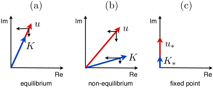
Figure 6: Location of the couplings in the Langevin equation (99) in the complex plane. Real (imaginary) parts describe reversible (irreversible) contributions to the dynamics. (a) An equilibrium system is characterized by the location of couplings on a single ray, reflecting detailed balance. The irreversible dynamics is not independent of the underlying reversible Hamiltonian dynamics, but rather generated by it. (b) In contrast, in a driven non-equilibrium system, generically there is a spread in the location of couplings, because the reversible and dissipative dynamics have different physical origins. (c) Near a critical point in three dimensions, the couplings flow strongly with scale and approach the imaginary axis (decoherence). The RG fixed point is purely dissipative. (Figure adapted from Sieberer et al. (2013).)

Finally, we note that, while an explicit violation of the symmetry is present on the microscopic scales on which the quantum master equation (16) or the corresponding Keldysh action (27) provide a suitable description of the system, in several cases it has been found that driven-dissipative systems appear as approximately thermal at low frequencies Mitra et al. (2006); Wouters and Carusotto (2006); Diehl et al. (2008, 2010b); Dalla Torre et al. (2010); Mitra and Giamarchi (2011, 2012); Öztop et al. (2012); Dalla Torre et al. (2013). In driven-dissipative condensates in three spatial dimensions, this thermalization at low frequencies is particularly sharply reflected via the emergence of the thermal symmetry in the RG flow in this regime Sieberer et al. (2013, 2014), cf. Fig. 6 (c); this is discussed in more detail in Sec. IV. On the other hand, there are also cases where the opposite behavior occurs, and the non-equilibrium character becomes more pronounced as one coarse grains to the macroscale. This occurs in driven two dimensional systems, as explained in Sec. IV.

II.4.3 The Noether theorem in the Keldysh formalism

A global continuous symmetry of the Keldysh action is a transformation $T_{\alpha}$ of the fields $\Psi=\left(\psi_{+},\psi_{+}^{*},\psi_{-},\psi_{-}^{*}\right)^{T}$ that leaves the value of the action invariant, i.e.,

$$S[T_{\alpha}\Psi]=S[\Psi],$$ (102)

where $\alpha$ is a real time- and space independent parameter, and for $\alpha=0$ the transformation is the identity, $T_{0}=\mathbbm{1}$. The Noether theorem states that any such global continuous symmetry entails the existence of a current $j$ with components $j^{\mu},$ which obeys a continuity equation on average, i.e., $\langle\partial_{\mu}j^{\mu}\rangle=0$ (here and in the following summation over repeated indicies is implied), where $\partial_{0}=\partial_{t}$, and $\partial_{1,2,\dotsc d}$ are derivatives with respect to spatial coordinates. Then, the integral over space $\mathscr{Q}=\int_{\mathbf{x}}j^{0}$ — the Noether charge — is an integral of motion, and we have $\langle d\mathscr{Q}/dt\rangle=0$. In the following, we prove this relation, which states that $\mathscr{Q}$ is conserved on average, in the framework of the Keldysh formalism. We note however, that a global continuous symmetry implies the even stronger statement $d\mathscr{Q}/dt=0$ of conservation of $\mathscr{Q}$ on the operator level Zinn-Justin (2002).

In order to prove the Noether theorem, it is sufficient to consider infinitesimal transformations. Then, for $\alpha\ll 1$ we expand the transformation as

$$T_{\alpha}\Psi=\Psi+\alpha\mathfrak{G}\Psi+O(\alpha^{2}),$$ (103)

where $\mathfrak{G}$ is called the generator of the transformation. In general, $\mathfrak{G}$ is a $4\times 4$ matrix with derivative operators as entries. We consider specific examples below in Sec. II.4.4. In the following we assume that as in Eq. (30) the action $S$ can be written in terms of a Lagrangian density $\mathscr{L}$ as $S=\int_{t,\mathbf{x}}\mathscr{L}$, and that the Lagrangian density is a local function of the fields and their first derivatives with respect to time and space. This assumption is appropriate for most practical purposes.

In an expansion of the LHS of Eq. (102) in powers of $\alpha$, each coefficient has to vanish individually. The first-order contribution yields the relation

$$\int_{t,\mathbf{x}}\left(\frac{\partial\mathscr{L}}{\partial\Psi^{T}}\mathfrak{G}\Psi+\frac{\partial\mathscr{L}}{\partial\partial_{\mu}\Psi^{T}}\partial_{\mu}\mathfrak{G}\Psi\right)=0,$$ (104)

where $\partial\mathscr{L}/\partial\Psi\equiv\left(\partial\mathscr{L}/\partial\psi_{+},\partial\mathscr{L}/\partial\psi_{+}^{*},\partial\mathscr{L}/\partial\psi_{-},\partial\mathscr{L}/\partial\psi_{-}^{*}\right)^{T}.$ In the cases we consider, Eq. (104) holds true because the integrand can be written as the divergence of a vector field $f^{\mu}$, i.e., we have

$$\partial_{\mu}f^{\mu}=\frac{\partial\mathscr{L}}{\partial\Psi^{T}}\mathfrak{G}\Psi+\frac{\partial\mathscr{L}}{\partial\partial_{\mu}\Psi^{T}}\partial_{\mu}\mathfrak{G}\Psi.$$ (105)

To proceed we consider local transformations, i.e., we consider $T_{\alpha}$ with $\alpha=\alpha(t,\mathbf{x})$. We perform a change of integration variables $\Psi\to T_{\alpha}\Psi$ in the partition function. Then, assuming that the functional measure is invariant with respect to the local transformation, we have

$$Z=\int\mathscr{D}[\Psi]e^{iS[\Psi]}=\int\mathscr{D}[\Psi]e^{iS[T_{\alpha}\Psi]}.$$ (106)

As before, we expand the RHS of this equality in a power series in $\alpha$. Since by assumption the latter is a function of $\left(t,\mathbf{x}\right)$, Eq. (102) does not hold true any more. Instead, we find

$$S[T_{\alpha}\Psi]=S[\Psi]+\int_{t,\mathbf{x}}\alpha\partial_{\mu}\left(f^{\mu}-\frac{\partial\mathscr{L}}{\partial\partial_{\mu}\Psi^{T}}\mathfrak{G}\Psi\right)+O(\alpha^{2}),$$ (107)

where we used Eq. (105) and integration by parts to write the RHS in a form that does not contain derivatives of $\alpha$ explicitly. Inserting Eq. (107) in the exponential on the RHS of Eq. (106), and expanding the latter to first order in $\alpha$, we obtain the condition

$$\int_{t,\mathbf{x}}\alpha\partial_{\mu}\left\langle f^{\mu}-\frac{\partial\mathscr{L}}{\partial\partial_{\mu}\Psi^{T}}\mathfrak{G}\Psi\right\rangle=0.$$ (108)

Since there are no restrictions on the choice of $\alpha$, this equation implies that the divergence of the expectation value vanishes. The latter is just the quantum Noether current,

$$j^{\mu}=\frac{\partial\mathscr{L}}{\partial\partial_{\mu}\Psi^{T}}\mathfrak{G}\Psi-f^{\mu}.$$ (109)

Note that $j^{\mu}$ is not unique: for constant $a,b^{\mu}$, the combination $aj^{\mu}+b^{\mu}$ is also a conserved current. The associated Noether charge $\mathscr{Q}$ corresponds to the integral over space of the zeroth component of the Noether current,

$$\mathscr{Q}=\int_{\mathbf{x}}j^{0}=\int_{\mathbf{x}}\left(\frac{\partial\mathscr{L}}{\partial\partial_{t}\Psi^{T}}\mathfrak{G}\Psi-f^{0}\right).$$ (110)

While this derivation is quite general, a more concrete expression for the Noether current can be obtained by restricting the form of the generator $\mathfrak{G}$ in Eq. (103). In particular, in the next section we consider the specific cases of classical and quantum transformations.

II.4.4 Closed systems: energy, momentum and particle number conservation

Energy and momentum conservation – This property is expected for systems, whose classical action is determined by a translationally invariant Hamiltonian alone. Indeed, the construction of the Keldysh action for a Markovian master equation in Sec. II.1 shows that terms which couple the forward and backward branches are only contained in the dissipative parts of the action (30). In other words, they arise upon coupling the system to a bath and integrating out the latter. On the other hand, the Keldysh action for a closed system with unitary dynamics does not contain such terms and can be written as

$$S=\sum_{\sigma}\sigma\int_{t,\mathbf{x}}\mathscr{L}_{\sigma},$$ (111)

where $\mathscr{L}_{+}$ and $\mathscr{L}_{-}$ are the Lagrangian densities evaluated with fields on the forward and backward branches, respectively. Given this structure of the action, let us consider a transformation $T_{\alpha}$ which does not mix fields on the forward and backward branches. Then, the generator $\mathfrak{G}$ has the block-diagonal structure

$$\mathfrak{G}=\begin{pmatrix}\mathfrak{g}_{+}&0\\ 0&\mathfrak{g}_{-}\end{pmatrix}.$$ (112)

The cases of physical interest are the classical and quantum transformations mentioned above, corresponding to the choices $\mathfrak{g}_{+}=\mathfrak{g}_{-}$ and $\mathfrak{g}_{+}=-\mathfrak{g}_{-}$, respectively. In both cases, the Noether current can be represented as superposition of currents on the forward and backward branches, which we define in terms of $\mathfrak{g}\equiv\mathfrak{g}_{+}$ as

$$j_{\sigma}^{\mu}=\frac{\partial\mathscr{L}_{\sigma}}{\partial\partial_{\mu}\Psi_{\sigma}^{T}}\mathfrak{g}\Psi_{\sigma}-f_{\sigma}^{\mu},$$ (113)

where

$$\partial_{\mu}f_{\sigma}^{\mu}=\frac{\partial\mathscr{L}_{\sigma}}{\partial\Psi_{\sigma}^{T}}\mathfrak{g}\Psi_{\sigma}+\frac{\partial\mathscr{L}_{\sigma}}{\partial\partial_{\mu}\Psi_{\sigma}^{T}}\partial_{\mu}\mathfrak{g}\Psi_{\sigma}.$$ (114)

With this definition, $j_{-}$ can be obtained from $j_{+}$ simply by replacing all instances of $\Psi_{+}$ appearing in $j_{+}$ by $\Psi_{-}$. Then, the symmetry of the action under a quantum transformation yields a classical Noether current and vice versa. These currents are given by (as noted above we are free to choose a convenient multiplicative normalization of the currents)

$$j_{c}=\frac{1}{2}\left(j_{+}+j_{-}\right),\quad j_{q}=j_{+}-j_{-}.$$ (115)

As pointed out in Sec. II.2.2, due to causality only the classical component of the field can acquire a finite expectation value. The same is true for the currents defined in Eq. (115): in the presence of an external field that induces a current, we have $\langle j_{+}\rangle=\langle j_{-}\rangle=\langle j_{c}\rangle\neq 0,$ whereas $\langle j_{q}\rangle=0.$ Hence, as anticipated above, the continuity equation $\langle\partial_{\mu}j^{\mu}_{q}\rangle=0$, which follows from the symmetry under a classical transformation, does not entail a non-trivial Noether charge. In the next section, we show that such a symmetry nevertheless does have physical consequences, as it can be broken spontaneously in a condensation transition.

Before, let us derive the Noether charge associated with the symmetry of a Hamiltonian Keldysh action under contour-dependent — i.e., quantum – translations in space-time. To be specific, we consider the transformation $\Psi_{\sigma}(X)\mapsto\Psi_{\sigma}(X+\sigma\alpha e_{\nu})$, where $X=\left(t,\mathbf{x}\right)$, and $e_{\nu}$ is the basis vector in direction of the $\nu$th coordinate of $d+1$-dimensional space-time. This is a symmetry of the action (111): the shift of the coordinates can be absorbed by performing a change of integration variables $X\to X-\sigma\alpha e_{\nu}$ in the integral over the Lagrangian density $\mathscr{L}_{\sigma}$. Clearly, the symmetry is violated in the presence of dissipative terms that couple the forward and backward branches.

For space-time translations, the generators $\mathfrak{g}_{\pm}$ in Eq. (112) acquire an additional index $\nu$ and are given by $\mathfrak{g}_{\pm,\nu}=\pm\partial_{\nu}$. It follows that the vector field $f_{\sigma,\nu}^{\mu}$ in Eq. (114) takes the form $f_{\sigma,\nu}^{\mu}=\delta^{\mu}_{\nu}\mathscr{L}_{\sigma}$, and the classical Noether current, which we denote as $T_{c,\nu}$, is given by

$$T_{c,\nu}^{\mu}=\frac{1}{2}\sum_{\sigma}T^{\mu}_{\sigma,\nu},\quad T^{\mu}_{\sigma,\nu}=\frac{\partial\mathscr{L}_{\sigma}}{\partial\partial_{\mu}\Psi_{\sigma}^{T}}\partial_{\nu}\Psi_{\sigma}-\delta^{\mu}_{\nu}\mathscr{L}_{\sigma},$$ (116)

where $T_{\pm,\nu}^{\mu}$ are the components of the energy-momentum tensor Zinn-Justin (2002); Peskin and Schroeder (1995) on the forward and backward branches. In particular, the component $T_{\pm,0}^{0}$ is the energy density, whereas $T_{\pm,i}^{0}$ is the density of momentum in the spatial direction $i=1,2,\dotsc,d$. The spatial integrals over these densities yield the associated Noether charges, e.g., if we express the Lagrangian density $\mathscr{L}_{\sigma}$ in terms of a Hamiltonian density (as in Eq. (30), where $\mathcal{L}$ is given by Eq. (28) with $\gamma_{\alpha}=0$) as

$$\mathscr{L}_{\sigma}=\frac{1}{2}\Psi_{\sigma}^{\dagger}i\sigma_{z}\partial_{t}\Psi_{\sigma}-H_{\sigma},$$ (117)

we obtain the conserved energy density $\mathscr{E}$, which is as expected given by the sum of the Hamiltonian densities on the forward and backward branches,

$$\mathscr{E}=\frac{1}{2}\sum_{\sigma}\int_{\mathbf{x}}T_{\sigma,0}^{0}=\frac{1}{2}\int_{\mathbf{x}}\left(H_{+}+H_{-}\right).$$ (118)

Along the same lines, conservation of angular momentum follows from the quantum symmetry of the Keldysh action with respect to rotations of the spatial coordinates.

Number conservation – As another example, we consider phase rotations and their relation to particle number conservation. In this case the classical transformation reads $\psi_{\pm}\mapsto U_{c}\psi_{\pm}=e^{i\alpha}\psi_{\pm}$ and the quantum transformation is $\psi_{\pm}\mapsto U_{q}\psi_{\pm}=e^{\pm i\alpha}\psi_{\pm}$. Classical phase rotations are a symmetry of the Keldysh action, if the fields appear only in the combinations $\psi_{\sigma}^{*}\psi_{\sigma^{\prime}}$. The quantum transformation is more restrictive: in this case only products with $\sigma=\sigma^{\prime}$ are allowed. Hence, the symmetry with regard to quantum phase rotations implies the classical symmetry. The generators of $U_{q}$ are given by $\mathfrak{g}_{\pm}=\pm i\sigma_{z}$. Then, with Eq. (10) and inserting the representation of the Lagrangian density in Eq. (117) in the expression for the Noether current (113), we find that the latter can be written as $j_{\sigma}=\left(\rho_{\sigma},\mathbf{j}_{\sigma}\right)^{T},$ where $\rho_{\sigma}=\left\lvert\psi_{\sigma}\right\rvert^{2}$ is the density on the contour with index $\sigma$ and the spatial components of the current are given by

$$\mathbf{j}_{\sigma}=\frac{1}{i2m}\left(\psi_{\sigma}^{*}\nabla\psi_{\sigma}-\psi_{\sigma}\nabla\psi_{\sigma}^{*}\right),$$ (119)

which is just the ordinary quantum mechanical current for particles with quadratic dispersion relation, evaluated on the closed time path. What is the physical meaning of the classical and quantum components, which are defined in Eq. (115), of the current given in Eq. (119)? If we introduce in the Hamiltonian an externally imposed gauge field, in the Keldysh action it would couple to the quantum current, in analogy to the source terms in the generating functional Eq. (33). However, the observable effect of such a gauge field is that it can induce a classical current $\langle j_{c}\rangle\neq 0$.

We close this section with a comment on the status of the $U_{q}(1)$ symmetry. It will be present on the microscopic level for an action corresponding to a Hamiltonian which commutes with the number operator. Since the symmetry considerations are properly applied to the microscopic action (and the functional measure), the conservation law ensues. However, this does not imply that the effective action must manifestly preserve a $U_{q}(1)$ symmetry. In fact, classical models of number conserving dynamics Hohenberg and Halperin (1977) do not exhibit this symmetry. This leads to the picture that this symmetry is broken spontaneously under RG. The precise workings of such a mechanism are, to the best of our knowledge, not settled so far.

II.4.5 Extended continuity equation in open systems

The conservation of particle number in a closed system follows from the continuity equation for the classical Noether current that is associated with the symmetry under quantum phase rotations. In an open system, this symmetry is absent, and the continuity equation has to be extended to account for the exchange of particles with the environment, as we discuss in the following.

To be specific, we consider the Keldysh action (73) for a system with single-particle pump as well as single-particle and two-body loss. In order to derive the extended continuity equation, as in Eq. (106) we perform a change of integration variables $\Psi\to U_{q}\Psi$, where $U_{q}$ is a local quantum phase rotation, in the Keldysh partition function. Since the partition function is invariant under this transformation, the coefficients in an expansion of the partition function in powers of the phase shift must vanish. In linear order, we find the condition

$$\langle\partial_{\mu}j_{c}^{\mu}\rangle-\gamma_{p}\langle\psi_{+}^{*}\psi_{-}\rangle+\gamma_{l}\langle\psi_{-}^{*}\psi_{+}\rangle+4u_{d}\langle\left(\psi_{-}^{*}\psi_{+}\right)^{2}\rangle=0.$$ (120)

This should be compared to Eq. (108): if $U_{q}$ were a symmetry of the action, we would have found an ordinary continuity equation. This would have been the case in the absence of the pumping and loss terms proportional to $\gamma_{p},\gamma_{l},$ and $u_{d}$. The interpretation of these terms is as follows: in a system that is perfectly isolated from its environment, the temporal change of the density at a given point is due to the motion of particles towards to or away from this point, i.e., the rate of change of density is a source or sink for the mass flow as measured by the divergence of the current $\langle\nabla\cdot\mathbf{j}_{c}\rangle$. In an open system, on the other hand, there is in addition a dissipative current Gebauer and Car (2004); Avron et al. (2012) due to the exchange of particles between the system and its environment. In particular, in Eq. (120) this dissipative current has contributions from the pumping and loss terms.

It is interesting to note that Eq. (120) can also be obtained from the equation of motion of the local density $n(\mathbf{x})=\psi^{\dagger}(\mathbf{x})\psi(\mathbf{x})$ in the operator formalism. From the master equation $\partial_{t}\rho=\mathcal{L}\rho$ with Liouvillian $\mathcal{L}$ in Lindblad form given in Eq. (9), it follows that the time evolution of $n(t,\mathbf{x})$ in the Heisenberg representation is given by $\partial_{t}n(t,\mathbf{x})=\mathcal{L}^{*}n(t,\mathbf{x})$ with the adjoint Liouvillian defined by $\mathop{\mathrm{tr}}(A\mathcal{L}B)=\mathop{\mathrm{tr}}(B\mathcal{L}^{*}A)$. We find

$$\partial_{t}n(t,\mathbf{x})=-\nabla\cdot\mathbf{j}(t,\mathbf{x})+\gamma_{p}\psi(t,\mathbf{x})\psi^{\dagger}(t,\mathbf{x})\\ -\gamma_{l}n(t,\mathbf{x})-4u_{d}\psi^{\dagger}(t,\mathbf{x})^{2}\psi(t,\mathbf{x})^{2},$$ (121)

where first term encodes coherent dynamics and corresponds to the Heisenberg commutator $i[H_{\mathrm{LP}},n(t,\mathbf{x})]$, whereas the remaining contributions incorporate the dissipative parts. Taking the average of this relation and expressing the expectation values as Keldysh functional integrals yields Eq. (120).

Finally, we can obtain some intuition on the dissipative correction to the current expectation value in mean field theory, where the correlators in Eq. (120) factorize into products of single field expectation values $\left\langle\psi_{+}\right\rangle=\left\langle\psi_{-}\right\rangle=\psi_{0}$. We then recognize in the non-derivative terms ($\psi_{0}^{*}$ times) the LHS of Eq. (75) (note that due to the factor of $1/\sqrt{2}$ in the Keldysh rotation (32) the expectation values are related as $\left\langle\phi_{c}\right\rangle=\phi_{0}=\sqrt{2}\left\langle\psi_{\pm}\right\rangle$, and that $r_{d}=(\gamma_{l}-\gamma_{p})/2$), which equals zero in a homogeneous situation within mean field theory. In this way, we see that there is no particle number current on average in a homogeneous driven-dissipative system in stationary state, as expected.

II.4.6 Spontaneous symmetry breaking and the Goldstone theorem

Even though the pumping and loss terms in the Keldysh action in Eq. (73) break the symmetry with respect to quantum phase rotations $U_{q}$, the action is still symmetric under $U_{c}$ transformations. As a result, even in the absence of particle number conservation there is a possibility of spontaneous symmetry breaking. In particular, a finite average value $\langle\phi_{c}\rangle\neq 0$ breaks the classical phase rotation symmetry in a non-equilibrium condensation transition. Here we show that this spontaneous symmetry breaking is accompanied by the appearance of a massless mode, i.e., a mode with vanishing frequency and decay rate for zero momentum, which is known as the Goldstone boson Goldstone (2008); Goldstone et al. (1962); Nambu and Jona-Lasinio (1961). We obtain this result by carrying over the corresponding derivation from the equilibrium formalism (see, e.g., Ref. Amit and Martin-Mayor (2005)) to the Keldysh framework.

The single-particle excitation spectrum is encoded in the poles of retarded and advanced Green’s functions, and such a pole at $\omega=q=0$ is dubbed a massless mode. Poles of the Green’s functions correspond to roots of the determinant of inverse propagator (see Sec. II.1). Hence, the presence of a massless mode can be detected by checking whether the determinant of the mass matrix $M$ vanishes. The latter is determined by the inverse propagator

$$P(\omega,\mathbf{q})=\begin{pmatrix}0&P^{A}(\omega,\mathbf{q})\\ P^{R}(\omega,\mathbf{q})&P^{K}(\omega,\mathbf{q})\end{pmatrix}=G^{-1}(\omega,\mathbf{q}),$$ (122)

given exemplarily in Eq. (76), at $\omega=\mathbf{q}=0$, i.e., $M=-P(0,0)$. Therefore, it is sufficient to consider frequency- and momentum-independent field configurations or, in other words, homogeneous field configurations, so that instead of the full effective action Eq. (39) we only have to deal with the effective potential $U=-\left.\Gamma\right\rvert_{\mathrm{hom.}}/\Omega$, where $\Omega$ is the quantization volume in space-time. Since the effective potential $U$ inherits the symmetries of the effective action, it is a function of precisely these combinations of fields which are invariant under classical or quantum phase rotations. In the basis of classical and quantum fields, these $U_{c}$-symmetric combinations are $\rho_{\nu\nu^{\prime}}=\phi_{\nu}^{*}\phi_{\nu^{\prime}}$, where the indices $\nu$ and $\nu^{\prime}$ can take the values $c$ and $q$. In the following, we show that $U_{c}$ invariance is sufficient to guarantee the existence of a massless mode.

For convenience we switch to a basis of real fields $\chi=(\chi_{c,1},\chi_{c,2},\chi_{q,1},\chi_{q,2})$ which correspond to the real and imaginary parts of the complex classical and quantum fields, i.e., $\phi_{\nu}=\frac{1}{\sqrt{2}}\left(\chi_{\nu,1}+i\chi_{\nu,2}\right)$ for $\nu=c,q$. In this basis, the mass matrix reads

$$M_{ij}=\left.\frac{\partial^{2}U}{\partial\chi_{i}\partial\chi_{j}}\right\rvert_{\mathrm{ss}}=\sum_{a}\left[\frac{\partial^{2}\rho_{a}}{\partial\chi_{i}\partial\chi_{j}}\frac{\partial U}{\partial\rho_{a}}\right]_{\mathrm{ss}}+\sum_{a,b}\left[\frac{\partial\rho_{a}}{\partial\chi_{i}}\frac{\partial\rho_{b}}{\partial\chi_{i}}\frac{\partial^{2}U}{\partial\rho_{a}\partial\rho_{b}}\right]_{\mathrm{ss}},$$ (123)

where the subscript $\mathrm{ss}$ indicates that the fields should be set to their average values in the stationary state. The indices $i$ and $j$ label the components of the four-vector $\chi$ defined above (i.e., $\chi_{1}=\chi_{c,1}$, $\chi_{2}=\chi_{c,2}$ etc.), and $a$ and $b$ are double indices, taking the values $cc,cq,qc,qq$. Let us consider the first term on the RHS of Eq. (123): in the ordered phase, the classical field has a finite expectation value in the stationary state. Without loss of generality we assume that this value is real. Then, the field equations

$$\left.\frac{\partial U}{\partial\chi_{i}}\right\rvert_{\mathrm{ss}}=\sum_{a}\left[\frac{\partial\rho_{a}}{\partial\chi_{i}}\frac{\partial U}{\partial\rho_{a}}\right]_{\mathrm{ss}}=0,$$ (124)

which actually determine the average value of the fields $\chi_{i}$ in stationary state, have the solution $\left.\chi_{i}\right\rvert_{\mathrm{ss}}=\sqrt{2\rho_{0}}\delta_{i,1}$. Performing the derivatives $\partial\rho_{a}/\partial\chi_{i}$ in Eq. (124) explicitly and inserting $\left.\chi_{i}\right\rvert_{\mathrm{ss}}$, we obtain the following conditions:

$$\left.\frac{\partial U}{\partial\rho_{cc}}\right\rvert_{\mathrm{ss}}=\left.\frac{\partial U}{\partial\rho_{cq}}\right\rvert_{\mathrm{ss}}=\left.\frac{\partial U}{\partial\rho_{qc}}\right\rvert_{\mathrm{ss}}=0.$$ (125)

Therefore, only the derivative $u_{qq}=[\partial U/\partial\rho_{qq}]_{\mathrm{ss}}$ contributes to the first term on the RHS of Eq. (123). Denoting mixed second derivatives of the effective potential as $u_{ab}=u_{ba}=[\partial^{2}U/\partial\rho_{a}\partial\rho_{b}]_{\mathrm{ss}}$, we find that the mass matrix can be written as

$$M=\begin{pmatrix}0&0&0&0\\ 0&0&0&0\\ 0&0&u_{qq}&0\\ 0&0&0&u_{qq}\end{pmatrix}+\rho_{0}\begin{pmatrix}0&0&u_{cc,cq}+u_{cc,qc}&i\left(u_{cc,cq}-u_{cc,qc}\right)\\ 0&0&0&0\\ u_{cc,cq}+u_{cc,qc}&0&\tfrac{1}{2}\left(u_{cq,cq}+2u_{cq,qc}+u_{qc,qc}\right)&\tfrac{i}{2}\left(u_{cq,cq}-u_{qc,qc}\right)\\ i\left(u_{cc,cq}-u_{cc,qc}\right)&0&\tfrac{i}{2}\left(u_{cq,cq}-u_{qc,qc}\right)&-\tfrac{1}{2}\left(u_{cq,cq}-2u_{cq,qc}+u_{qc,qc}\right)\\ \end{pmatrix}.$$ (126)

An entry $u_{cc,cc}$ is not ruled out by symmetry, however, it must vanish due to conservation of probability, cf. Sec. II.2.1. Crucially, the retarded and advanced sectors feature one zero eigenvalue. This proves the existence of a massless mode as a consequence of spontaneous symmetry breaking for a theory with $U_{c}$ invariance.

While this analysis guarantees the existence of a zero mode (i.e., the complex dispersion relation has the property $\omega(q=0)=0$), it does not provide a statement on the functional dependence $\omega(q)$. The latter could be inferred along the lines of Refs. Minami and Hidaka (2015); Watanabe and Murayama (2012); Hidaka (2013); Watanabe and Murayama (2014); Hayata and Hidaka (2015). As we found in Sec. II.2.2 in Bogoliubov approximation, in an open system without (i.e., broken) $U_{q}$ symmetry and spontaneously broken $U_{c}$ symmetry, the leading behavior at low momenta is diffusive, $\omega(q)\sim-iDq^{2}$, with a real diffusion coefficient $D$. This has to be contrasted to closed systems, in which microscopically both $U_{q}$ and $U_{c}$ symmetry are present. There, the leading behavior in a phase with spontaneously broken $U_{c}$ symmetry is that of coherent sound waves, $\omega(\mathbf{q})\sim cq$, with real speed of sound $c$. A phenomenological justification of this behavior is given in Ref. Hohenberg and Halperin (1977), where this can be understood as a consequence of a coupling to additional slow modes relating to particle number conservation. In these phenomenological models, $U_{q}$ symmetry is absent. This suggests a scenario of an additional spontaneous breakdown of $U_{q}$ symmetry upon coarse graining, but this issue seems not to be settled to date.

II.5 Open system functional renormalization group

In Sec. IV.2, we investigate dynamical criticality of the Bose condensation transition in driven open systems, motivated by many-body ensembles such as exciton-polariton condensates Kasprzak et al. (2006); Snoke (2008); Wouters and Carusotto (2007a); Szymańska et al. (2006); Carusotto and Ciuti (2013). There again, coherent dynamics naturally competes with dissipation in the form of incoherent particle losses and pumping. The situation parallels a laser threshold Graham and Haken (1970); DeGiorgio and Scully (1970), however with a continuum of spatial degrees of freedom. This ingredient, however, causes the characteristic long-wavelength divergences of many-body problems in their symmetry broken phase, or at a critical point. It implies that perturbation theory necessarily breaks down, even when the interaction constants are small, due to a continuum of modes without a gap, which form the intermediate states and are summed over in many-body perturbation theory. This calls for the development of efficient functional integral techniques able to cope with these problems. Our method of choice is the functional renormalization group based on the Wetterich equation Wetterich (1993), which we briefly introduce here in its Keldysh formulation. This approach offers the particularly attractive feature of not being restricted to the critical point.

The functional renormalization group equation (for reviews see Berges et al. (2002); Delamotte (2012); Blaizot et al. (2006); Pawlowski (2007); Boettcher et al. (2012)) constitutes an exact reformulation of the functional integral representation of a quantum many-body problem in terms of a functional differential equation. In this, it is strongly distinct from, e.g., perturbative field theoretical renormalization group approaches, which concentrate exclusively on the critical surface of a given problem. Instead, it may be viewed as an alternative and potentially more tractable tool for the analysis of the complete many-body problem, also on length scales well below the correlation length near criticality. Indeed, it has proven a very versatile tool in many different physical context, ranging from quantum dots Jakobs et al. (2007, 2010b); Karrasch et al. (2010), ultracold atoms Boettcher et al. (2012), strongly correlated electrons Metzner et al. (2012), classical stochastic models Canet and Chaté (2007); Mesterházy et al. (2013), quantum chromodynamics Pawlowski (2007); Rosten (2012), to quantum gravity Reuter (1998). Here we give a brief overview of the general concept adapted to non-equilibrium systems Gezzi et al. (2007); Karrasch et al. (2010); Jakobs et al. (2007, 2010b); Berges et al. (2008); Berges and Hoffmeister (2009); Berges and Mesterházy (2012); Gasenzer and Pawlowski (2008); Sieberer et al. (2013, 2014); Canet et al. (2004a, 2005); Canet (2006); Canet et al. (2004b, 2011a, 2010, 2011b, 2012). It is used for the discussion of critical behavior in driven open quantum systems in Sec. IV, with applications to a broader non-equilibrium many-body context left for future work.

The transition from the action $S$ to the effective action $\Gamma$ consists in the inclusion of both statistical and quantum fluctuations into the latter (cf. Eq. (39)). In the functional renormalization group approach based on the Wetterich equation Wetterich (1993), the functional integral over fluctuations is carried out stepwise. To this end, an infrared regulator is introduced, which suppresses the fluctuations with momenta less than an infrared cutoff scale $\Lambda$. This is achieved by adding to the action in (33) a term

$$\Delta S_{\Lambda}=\int_{t,\mathbf{x}}\left(\phi_{c}^{*},\phi_{q}^{*}\right)\begin{pmatrix}0&R_{\Lambda}\\ R_{\Lambda}^{*}&0\end{pmatrix}\begin{pmatrix}\phi_{c}\\ \phi_{q}\end{pmatrix},$$ (127)

with a cutoff or regulator function $R_{\Lambda}$. Some key structural properties are indicated below, but apart from these properties the choice of the cutoff is flexible and problem-specific. The resulting cutoff-dependent generating functional and its logarithm (cf. Eq. (35)) are denoted by, respectively, $Z_{\Lambda}$ and $W_{\Lambda}$. Then, the scaled-dependent effective action $\Gamma_{\Lambda}$ is defined by modifying the Legendre transform in Eq. (38) according to

$$\Gamma_{\Lambda}[\bar{\Phi}_{c},\bar{\Phi}_{q}]=W_{\Lambda}[J_{c},J_{q}]\\ -\int_{t,\mathbf{x}}\left(J_{c}^{\dagger}\bar{\Phi}_{q}+J_{q}^{\dagger}\bar{\Phi}_{c}\right)-\Delta S_{\Lambda}[\bar{\Phi}_{c},\bar{\Phi}_{q}].$$ (128)

The subtraction of the $\Delta S_{\Lambda}$ on the RHS guarantees that the only difference between the functional integral representations for $\Gamma$ and $\Gamma_{\Lambda}$ is the inclusion of the cutoff term in the latter,

$$e^{i\Gamma_{\Lambda}[\bar{\Phi}_{c},\bar{\Phi}_{q}]}=\int\mathscr{D}[\delta{\Phi}_{c},\delta{\Phi}_{q}]\,e^{iS[\bar{\Phi}_{c}+\delta{\Phi}_{c},\bar{\Phi}_{q}+\delta{\Phi}_{q}]}\\ \times e^{-i\tfrac{\delta\Gamma}{\delta\bar{\Phi}_{c}^{T}}\delta{\Phi}_{q}-i\tfrac{\delta\Gamma}{\delta{\Phi}_{q}^{T}}\delta{\Phi}_{c}+i\Delta S_{\Lambda}[\delta{\Phi}_{c},\delta{\Phi}_{q}]}.$$ (129)

Physically, $\Gamma_{\Lambda}$ can thus be viewed as the effective action for averages of fields over a coarse-graining volume with a size $\sim\Lambda^{-d}$, where $d$ is the spatial dimension.

Note that we chose the form of the cutoff action $\Delta S_{\Lambda}$ such that it modifies the inverse retarded and advanced propagators in Eq. (127) only. This is sufficient to regularize possible infrared divergences, which result from poles of the retarded and advanced propagators being located at the origin of the complex frequency plane. A typical choice in practical calculations is

$$R_{\Lambda}(q^{2})\sim\Lambda^{2},\quad q/\Lambda\to 0,$$ (130)

giving the inverse propagators a mass $\sim\Lambda^{2}$. In this way, fluctuations with wavelength $\gtrsim\Lambda^{-1}$ are effectively cut off. Therefore, for any finite $\Lambda$, the technical problem of infrared divergences is under control.

The main usefulness of the so-modified effective action, however, lies in the fact that it smoothly interpolates between the action $S$ for $\Lambda\to\Lambda_{0}$, where $\Lambda_{0}$ is the ultraviolet cutoff of the problem (e.g., the inverse lattice spacing), and the full effective action $\Gamma$ for $\Lambda\to 0$. This is ensured by the following requirements on the cutoff Berges and Hoffmeister (2009):

$$R_{\Lambda}(q^{2}) \sim\Lambda_{0}^{2}, \Lambda \to\Lambda_{0},$$ (131)

$$R_{\Lambda}(q^{2}) \to 0, \Lambda \to 0.$$

Under the condition that $\Lambda_{0}$ exceeds all energy scales in the action, for $\Lambda\to\Lambda_{0}$ we may evaluate the functional integral (129) in the stationary phase approximation. Then, we find to leading order $\Gamma_{\Lambda_{0}}\sim S$ — in the absence of fluctuations (suppressed by the cutoff mass gap $\sim\Lambda_{0}^{2}$), the effective action approaches the classical, or microscopic one. The evolution of $\Gamma_{\Lambda}$ from this starting point in the ultraviolet to the full effective action in the infrared for $\Lambda\to 0$ is described by an exact flow equation — the Wetterich equation Wetterich (1993) — which was adapted to the Keldysh framework in Jakobs et al. (2007, 2010b); Gasenzer and Pawlowski (2008); Berges and Hoffmeister (2009). It reads

$$\partial_{\Lambda}\Gamma_{\Lambda}=\frac{i}{2}\mathop{\mathrm{Tr}}\left[\left(\Gamma^{(2)}_{\Lambda}+R_{\Lambda}\right)^{-1}\partial_{\Lambda}R_{\Lambda}\right],$$ (132)

where $\Gamma_{\Lambda}^{(2)}$ and $R_{\Lambda}$ denote, respectively the second variations of the effective action and the cutoff action $\Delta S_{\Lambda}$. As anticipated above, the flow equation provides us with an alternative but fully equivalent formulation of the functional integral (129) as a functional differential equation. Like the functional integral, the flow equation can not be solved exactly for most interesting problems. It is, however, amenable to numerous systematic approximation strategies. For example, in the vicinity of a critical point it is possible to perform an expansion of the effective action $\Gamma_{\Lambda}$ in terms canonical scaling dimensions, keeping only those couplings which are — in the sense of the renormalization group — relevant or marginal at the phase transition, cf. the discussion in Sec. II.3, and see Sec. IV.2 for applications.

Part 2 Applications

III Non-equilibrium stationary states: spin models

In this section, we discuss the steady state properties of many-body systems consisting of atoms, which are coupled to the radiation field of a cavity, in turn subject to dissipation in the form of permanent photon loss. The corresponding low frequency field theory, a $0+1$-dimensional path integral for real valued, Ising type fields corresponds to the simplest, non-trivial field theoretic models and is therefore particular useful to get used to applications of the Keldysh formalism for relevant physical setups. The basic model describing the dynamics of atoms in a cavity is the Dicke model (1) with dissipation, as described in Sec. I.3.1, as well as its extension to multiple cavity photon modes. Despite the simplicity of the underlying field theory, it is a non-trivial task to solve it for its rich many-body dynamics. This includes the critical behavior of a single mode cavity at the superradiance transition as well as universal dynamics in the formation of spin glasses in multi-mode cavities. We discuss these and further features of the Dicke model here by putting a focus on the theoretical framework of solving the corresponding Ising model on the Keldysh contour.

III.1 Ising spins in a single-mode cavity

As for the equilibrium path integral, the Keldysh field theory for spin models which obey the standard Ising $Z_{2}$ symmetry, is formulated in terms of real fields, fluctuating in time and space. These models have become rather important in the field of quantum optics, where the typical situation consists of a set of atoms, modeled as two-level systems, coupled to the radiation field of a high finesse cavity. One important model in this context is the Dicke model, which has been introduced in Eq. (1) as the generic model for cavity QED experiments with strong light-matter coupling. Its Hamiltonian is

$$H=\omega_{p}a^{\dagger}a+\frac{\omega_{z}}{2}\sum_{i=1}^{N}\sigma^{z}_{i}+\frac{g}{\sqrt{N}}\sum_{i=1}^{N}\sigma^{x}_{i}\left(a^{\dagger}+a\right).$$ (133)

The Dicke Hamiltonian represents an effective model which describes the dynamics of a set of two-level atoms, labeled by the index $i$, inside a cavity, which is pumped by a transverse laser. In this scenario, the coupling constant $g$ describes the scattering of laser photons into the cavity, as well as the reverse process, and therefore rotates in time with the laser frequency $\omega_{l}$. In a rotating frame, this time dependence is gauged away in the Hamiltonian, resulting in an effective shift $\omega_{p}=\omega_{c}-\omega_{l}$ of the bare cavity frequency $\omega_{c}$. In addition to this external drive, the cavity is subject to permanent photon loss, due to imperfections in the cavity mirrors. The photon loss is described by a weak coupling of the intra-cavity photons to the environment, i.e., the vacuum radiation field outside the cavity. For typical experimental parameters, this coupling, which represents the rate with which the intra-cavity field and the environment exchange photons, is much smaller than the typical relaxation time of the environment and the latter can be traced out under the Born and Markov approximation. This results in a Markovian master equation for the system’s density matrix, which reads (cf. Eqs. (2,16) repeated for convenience)

$$\partial_{t}\rho=-i[H,\rho]+\mathcal{L}\rho.$$ (134)

In this equation, $\rho$ is the density matrix, $H$ is the Dicke Hamiltonian (133) and $\mathcal{L}$ is the dissipative Liouvillian, acting as on the density matrix as

$$\mathcal{L}\rho=\kappa\left(a\rho a^{\dagger}-\frac{1}{2}\{a^{\dagger}a,\rho\}\right)$$ (135)

with loss rate $\kappa$ for the cavity photons.

Given the Markovian master equation (134), there are two common ways to derive a corresponding path integral description for the dissipative Dicke model, which are based on different representations of the atomic degree of freedom in terms of field variables: the representation of the atomic degrees of freedom as a collective spin and subsequent bosonization in terms of a Holstein-Primakoff transformation Emary and Brandes (2003); Öztop et al. (2012); Kulkarni et al. (2013), and the representation of the atomic variables in terms of individual Ising fields. We discuss both approaches in the following, putting a focus on the more general Ising representation, which can also be applied in the case of multiple cavity modes and individual atomic loss processes, where a representation of the atoms in terms of a single, collective spin is no longer possible. In the regimes for which both approaches can be applied, they are completely equivalent, as we demonstrate.

III.1.1 Large-spin Holstein-Primakoff representation

The single-mode Dicke Hamiltonian (133) has the property that all atomic variables couple to the cavity photon mode via the same coupling constant $g$. Consequently, the coupling of the photons to the sum of the individual Pauli matrices can be replaced by the coupling of the cavity photon mode to a large spin,

$$H=\omega_{p}a^{\dagger}a+\omega_{z}S^{z}+\frac{2g}{\sqrt{N}}S^{x}\left(a^{\dagger}+a\right),$$ (136)

where $S^{z},S^{x}$ are spin operators in a spin-$N/2$ Hilbert space. In order to find a path integral representation for the Hamiltonian (136), these spin operators can be transformed into bosonic operators via the common Schwinger-boson or Holstein-Primakoff transformations. For weak coupling $g$, the system remains strongly polarized $|\langle S_{z}\rangle|\gg 1$ and the Holstein-Primakoff transformation around the non-interacting ground state, which has the eigenvalue $S_{z}=-N/2$, is the most natural choice. It reads

$$S^{z}=b^{\dagger}b-\frac{N}{2},\ \ \ S^{x}=\left(\sqrt{N-b^{\dagger}b}\right)b+b^{\dagger}\left(\sqrt{N-b^{\dagger}b}\right),$$ (137)

where $b,b^{\dagger}$ are bosonic operators. In the thermodynamic limit $N\rightarrow\infty$, the square root in the $S^{x}$ operator is expanded in powers of $1/N$, and the Hamiltonian is subsequently formulated on the Keldysh contour. To zeroth order in $1/N$, the corresponding Keldysh action is

$$S=\int_{\omega}\Phi^{\dagger}(\omega)\left(\begin{array}[]{cc}0&\left(G^{A}_{4\times 4}\right)^{-1}\\ \left(G^{R}_{4\times 4}\right)^{-1}&\Sigma^{K}_{4\times 4}\end{array}\right)\Phi(\omega),$$ (138)

with the combined Nambu-Keldysh spinor

$$\Phi(\omega)=\left(a_{c}(\omega),a^{*}_{c}(-\omega),b_{c}(\omega),b^{*}_{c}(-\omega),a_{q}(\omega),a^{*}_{q}(-\omega),b_{q}(\omega),b^{*}_{q}(-\omega)\right)^{T},$$ (139)

the inverse retarded Green’s function in Nambu space

$$\left(G^{R}_{4\times 4}\right)^{-1}=\left(\begin{array}[]{cccc}\omega-\omega_{p}+i\kappa&0&-g&-g\\ 0&-\omega-\omega_{p}-i\kappa&-g&-g\\ -g&-g&\omega-\omega_{z}&0\\ -g&-g&0&-\omega-\omega_{z}\end{array}\right)$$ (140)

and the Keldysh self-energy

$$\Sigma^{K}=2i\kappa\mbox{ diag}(1,1,0,0).$$ (141)

Due to the photon decay terms $\sim\kappa$ and the atom-photon coupling $g$, the above theory is regularized even without infinitesimal imaginary contributions in the atomic sector. When integrating out the photons, the latter infinitesimal contributions are overwritten in any case by the finite imaginary part of the photon Green’s function, and it is therefore reasonable to leave them out from the start.

The excitation spectrum of the atom-photon system is encoded in the retarded Green’s function, and the poles, marking the excitation energies, fulfill the requirement

$$0\overset{!}{=}\det\left(G^{R}_{4\times 4}\right)^{-1}=(\omega^{2}-\omega_{z}^{2})[(\omega+i\kappa)^{2}-\omega_{p}^{2}]-4g^{2}\omega_{p}\omega_{z}.$$ (142)

In the absence of atom-photon coupling, i.e., for $g=0$, these are the non-interacting poles $\omega_{1,2}=\pm\omega_{z}$, corresponding to the atomic transition frequencies and $\omega_{3,4}=\pm\omega_{p}+i\kappa$, corresponding to the energy of a photon $\omega_{p}$ and its decay rate $\kappa$. For $g>0$, the modes begin to hybridize and the excitation energies are slightly modified compared to their non-interacting values, see Fig. 7. For small coupling strength, the elementary excitations can still be seen as weakly dressed atoms and photons, with excitation energies close to the non-interacting values, while they strongly hybridized, inseparable degrees of freedom for strong coupling strengths.

Above a critical coupling strength $g_{c}$, the ground state of the system breaks the $Z_{2}$ symmetry and the atoms form a macroscopic spin aligned in the $x$-direction, $\langle S_{x}\rangle=O(N)$, which is accompanied with a coherent macroscopic population of the intra-cavity mode $\langle a\rangle\neq 0$. This symmetry broken phase is called the superradiant phase of the cavity system. In the case of a macroscopic expectation of $S_{x}$, the orthogonal $S_{z}$ component can no longer be macroscopically large, which renders any expansion of the Holstein-Primakoff operators (137) in $1/N$ invalid. This is expressed by an instability of the quadratic theory at the superradiance transition, revealed by the presence of a zero energy mode, i.e., a pole at $\omega=0$ in the excitation spectrum. According to Eq. (142), this happens at

$$g_{c}=\sqrt{\frac{(\kappa^{2}+\omega_{p}^{2})\omega_{z}}{4\omega_{p}}}.$$ (143)

The mode structure in the vicinity of the transition has been analyzed in Ref. Dalla Torre et al. (2013), where it has been found that in the presence of photon decay, the critical mode becomes purely imaginary before the transition happens, and the corresponding critical dynamics corresponds to a classical finite temperature transition, see also Fig. 7. This is mirrored by the fact that the photons effectively thermalize in the low energy regime and their correlations can be described by a low energy effective temperature $T_{\mbox{\tiny eff}}$. The effective temperature can be obtained via a fluctuation dissipation relation, as discussed in Eq. (72) but promoted to Nambu space (see Sec. V.2 for a discussion of the FDR in Nambu space). Solving this equation yields the photon distribution function in Nambu representation

$$F_{\mbox{\tiny ph}}=\sigma^{z}+\sigma^{x}\frac{2g^{2}}{\omega_{z}\omega}\frac{\omega_{z}^{2}}{\omega^{2}-\omega_{z}^{2}}.$$ (144)

For large frequencies $\omega\gg\frac{g^{2}}{\omega_{z}}$, this corresponds to the zero temperature distribution of the non-interacting system $F=\sigma^{z}$, which is diagonal in the photon modes. The approach to this limit is, however, algebraic $\sim\omega^{-3}$, in contrast to an exponential approach according to large frequency behavior of the Bose-distribution function in equilibrium. On the other hand, for small frequencies $\omega\ll\frac{g^{2}}{\omega_{z}}$, the occupation becomes essentially thermal and purely off-diagonal $F=\frac{2T_{\mbox{\tiny eff}}}{\omega}\sigma^{x}$, with low energy effective temperature $T_{\mbox{\tiny eff}}=\frac{g^{2}}{\omega_{z}}$, cf. Eq. (84). In this low frequency limit, the elementary excitations are strongly hybridized polariton modes, which are diagonal in the photon quadratures $x$ and $p$. The absence of a global temperature scale in the present system reflects the fact that due to the Markovian dissipation, this interacting system with a discrete set of degrees of freedom is not able to achieve detailed balance between the particular modes, i.e. the $x$ and $p$ quadratures, for all energy scales.

One should note that $T_{\mbox{\tiny eff}}$ is not proportional to the decay rate $\kappa$ and consequently the zero temperature equilibrium limit is not simply obtained by taking the limit $\kappa\rightarrow 0$. The reason is that in the present setting, the atom-photon coupling $g$ leads to a competition of unitary and dissipative dynamics, which is reflected in the fact that for $g=0$, the eigenstate of the Hamiltonian is a steady state of the dynamics while this is no longer the case for finite $g$. As a consequence, the low energy effective temperature depends on $g$ and vanishes in the limit $g\rightarrow 0$.

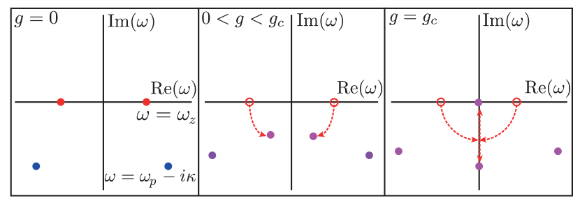
Figure 7: Illustration of the pole structure of the system’s eigenmodes. The poles represent the location of the mode frequencies $\omega$ in the complex plane, the real part $\text{Re}(\omega)$ represents the energy of the mode, while the imaginary part $\text{Im}(\omega)$ is the mode’s decay rate. Without interactions, $g=0$, the system is described by the bare atomic, $\omega=\pm\omega_{z}$, and photonic modes $\omega=\pm\omega_{p}-i\kappa$. For finite interactions, the atoms and photons hybridize and form polaritonic modes, two of which move closer to the imaginary axis. At the critical point $g=g_{c}$, one single mode becomes critical at $\omega=0$ and the system undergoes a phase transition from a disordered phase to the $Z_{2}$ symmetry breaking superradiant phase. The classical nature of the transition in the presence of dissipation is expressed by the fact that the two zero energy modes $\text{Re}(\omega)=0$ become purely dissipative for couplings $g<g_{c}$ already (indicated with the red arrows).

A further consequence of the dissipative nature of the transition is that the critical exponents correspond to the classical finite temperature equilibrium transition. One such critical exponent of the superradiant transition is the so-called photon flux exponent $\nu_{x}$, which describes the divergence of the cavity photon number at the transition, i.e., $n\sim|g-g_{c}|^{-\nu_{x}}$. It is obtained by frequency integration over the photonic correlation function

$$2n=\left(\int_{\omega}iG^{K}_{\mbox{\tiny ph}}(\omega)\right)-1\sim|g-g_{c}|^{-1}.$$ (145)

The exponent $\nu_{x}=1$ found for the present non-equilibrium transition coincides with the classical, finite temperature exponent for the equilibrium Dicke model in line with the discussion above. On the other hand, at zero temperature, the exponent of the corresponding quantum phase transition is found to be $\nu_{x}=1/2$.

The scaling behavior of the critical mode at the transition is expressed in terms of the dynamical critical exponent $\nu_{t}$. In the presence of dissipation, the excitations in the system decay exponentially in time, which results in an asymptotic exponential decay of real-time correlation functions

$$\langle\{a(t),a^{\dagger}(0)\}\rangle=G^{K}_{\mbox{\tiny ph}}(t)\sim e^{-t/\xi_{t}}.$$ (146)

The characteristic decay time $\xi_{t}$ is determined by the slowest decaying mode in the system, i.e., by the mode with the smallest imaginary part in the frequency spectrum. In the vicinity of the phase transition, this is the critical mode , which shows scaling

$$\xi_{t}\sim\frac{1}{|g-g_{c}|},$$ (147)

i.e., a dynamical critical exponent $\nu_{t}=1$. This behavior is in stark contrast to a zero temperature quantum phase transition, where correlation functions do not decay over time but oscillate with characteristic frequencies $\omega_{c}$, the smallest of which indicates the distance to the phase transition and encodes the critical scaling behavior. The fact that in the present setting the critical mode becomes purely imaginary is a generic feature of dissipative phase transitions, which is discussed further in Sec. IV.

All of the above discussed results are encoded in the quadratic Keldysh action, described by Eqs. (138-141). The resulting critical behavior is then that of a non-interacting system, and is associated accordingly to a Gaussian fixed point of the renormalization group flow. This is in contrast to critical behavior in interacting systems, which are described by an interacting Wilson-Fisher fixed point, not smoothly connected to the previous one (cf. the discussion in Sec. IV.2). This action describes the problem up to $1/N$ corrections resulting from the expansion of the Holstein-Primakoff bosons in $1/N$. It contains correctly the physics in the thermodynamic limit $N\rightarrow\infty$ and captures the essential dynamics of the superradiance transition. For finite systems, the higher order terms in $1/N$ can not be neglected and have to be taken into account properly. Analytical approaches, relying on an expansion of the Holstein-Primakoff operators up to first order in the ratio $1/N$, have shown that the first order correction term leads to a quartic contribution in the action, whose self-consistently determined one-loop corrections are already in very good agreement with numerical results Dalla Torre et al. (2013). The latter have been obtained from a Monte-Carlo wave function (MCWF) simulation of the master equation and agreed with the analytical results even on the level of $N=10$ atoms.

III.1.2 Effective Ising spin action for the single-mode cavity

The Dicke model defined by the master equation (134) obeys the common Ising $Z_{2}$ symmetry, which is spontaneously broken by the ground state of the superradiant phase. Another approach to express the Dicke model in a Keldysh path integral approach is therefore to represent the spin operators in terms of real Ising field variables, $\sigma_{x}(t)\rightarrow\phi(t)$. In contrast to the Holstein-Primakoff transformation applied in the previous section, the Ising representation does not require a single, large spin to have a well defined field theory representation, and is therefore also applicable in situations in which the atom-photon coupling is spatially dependent $g\rightarrow g(x)$ and a large spin representation becomes impossible. Furthermore, we use this approach to describe the symmetry broken phase of the problem.

The atomic sector of the Hamiltonian (133) describes Ising spins in a transverse field and the corresponding universal low energy description for frequencies below the level spacing $\omega_{z}$ is obtained by transforming the quantum spin operators to classical real fields. According to the quantum to classical mapping Kogut (1979) this is possible in the scaling regime of the corresponding, i.e., for the present case in the vicinity of the $2$nd order superradiance and glass transitions. The present model represents a generalization of the zero-dimensional Ising model in a transverse field, for which the quantum to classical mapping is known Kogut (1979) and consists of the replacements

$$\sigma^{x}_{i}(t)\rightarrow\phi_{i}(t)$$ (148)

and

$$\sigma^{z}_{i}(t)\rightarrow 1-\tfrac{2}{\omega_{z}^{2}}\left(\partial_{t}\phi_{i}(t)\right)^{2}.$$ (149)

The dynamic constraint $(\sigma^{x}_{i}(t))^{2}=1$ is implemented via the non-linear constraint

$$\delta(\phi_{i}^{2}(t)-1)=\int\mathcal{D}\lambda_{l}(t)\ e^{i\lambda_{l}(t)(\phi_{i}^{2}(t)-1)},$$ (150)

which introduces dynamical Lagrange parameters $\lambda_{i}(t)$ for each spin variable. In this framework, the purely atomic part of the action on the $(\pm)$-contour is

$$S_{\mbox{\tiny at}}=\tfrac{1}{\omega_{z}}\int_{\omega}\sum_{\alpha=\pm\atop i=1,..,N}\alpha\left[\lambda_{\alpha i}\left(\phi_{\alpha i}^{2}-1\right)-(\partial_{t}\phi_{\alpha i})^{2}\right].$$ (151)

The action for the atom-photon coupling and the bare photonic part is straightforwardly derived according to the previous sections, and the corresponding Keldysh action is

$$S=\frac{1}{\omega_{z}}\int_{t}\sum_{i}(\phi_{ci},\phi_{qi})\left(\begin{array}[]{cc}\lambda_{qi}(t)&\lambda_{ci}(t)+\partial_{t}^{2}\\ \lambda_{ci}(t)+\partial_{t}^{2}&\lambda_{qi}(t)\end{array}\right)\left(\begin{array}[]{c}\phi_{ci}\\ \phi_{qi}\end{array}\right)\\ +\frac{g}{\sqrt{N}}\int_{t}\sum_{i}\left(\phi_{ci}(a^{*}_{q}+a_{q})+\phi_{qi}(a^{*}_{c}+a_{c})\right)\\ +\int_{t}(a^{*}_{c},a^{*}_{q})\left(\begin{array}[]{cc}0&i\partial_{t}-\omega_{p}-i\kappa\\ i\partial_{t}-\omega_{p}+i\kappa&2i\kappa\end{array}\right)\left(\begin{array}[]{c}a_{c}\\ a_{q}\end{array}\right).$$ (152)

It is quadratic in the fields $\phi,a,a^{*}$ as it was the case for the Holstein-Primakoff action in the large-$N$ limit. However, the non-linear constraint, i.e., the fact that $\lambda_{q,c}$ is a dynamic variable, introduces higher order terms in the Ising fields. The approach corresponding to the large-$N$ expansion of the Holstein-Primakoff fields in the present formalism (in the sense that the action becomes quadratic) is to treat the Lagrange parameters as static mean field variables, i.e., $\lambda_{ci}(t)\rightarrow\lambda_{c}$ and $\lambda_{qi}(t)\rightarrow\lambda_{q}$. Due to causality, a static mean quantum field must be zero, $\lambda_{q}=0$. On the other hand, the value of $\lambda_{c}$ has to be chosen such that the non-linear constraint is preserved on average

$$\langle(\sigma^{x}_{i}(t))^{2}\rangle=\langle\phi_{c}^{2}(t)\rangle=\int_{\omega}iG^{K}_{\mbox{\tiny at}}(\omega)\overset{!}{=}1.$$ (153)

This is equivalent to a vanishing variation of the action with respect to the Lagrange parameters $\lambda_{c,q}$ and is known as the “soft-spin” approach to spin models (i.e. the constraint is treated on the mean field level). It becomes exact in the thermodynamic limit $N\rightarrow\infty$ Ye et al. (1993); Read et al. (1995).

Integrating out the $N$ individual atoms leads to the effective photon action

$$S=\frac{1}{2}\int_{\omega}A^{\dagger}(\omega)\left(\begin{array}[]{cc}0&\left(G^{A}_{2\times 2}\right)^{-1}\\ \left(G^{R}_{2\times 2}\right)^{-1}&2i\kappa\ \mbox{diag}(1,1)\end{array}\right)A(\omega),$$ (156)

with the Nambu spinor

$$A(\omega)=\left(\begin{array}[]{c}a_{c}(\omega)\\ a^{*}_{c}(-\omega)\\ a_{q}(\omega)\\ a^{*}_{q}(-\omega)\end{array}\right)$$ (161)

and the inverse retarded Green’s function

$$\left(G^{R}_{2\times 2}\right)^{-1}=\left(\begin{array}[]{cc}\omega-\omega_{p}+i\kappa-\frac{2g^{2}\omega_{z}}{\omega^{2}-\lambda}&-\frac{2g^{2}\omega_{z}}{\omega^{2}-\lambda}\\ -\frac{2g^{2}\omega_{z}}{\omega^{2}-\lambda}&\omega-\omega_{p}-i\kappa-\frac{2g^{2}\omega_{z}}{\omega^{2}-\lambda}\end{array}\right).$$ (162)

The poles of the Green’s function are again determined by the zeros of the determinant of the inverse Green’s function, i.e., by the roots of the equation

$$0\overset{!}{=}(\lambda_{c}-\omega^{2})\left((\omega+i\kappa)^{2}-\omega_{p}^{2}\right)+4\omega_{p}\omega_{z}g^{2}.$$ (163)

For the non-interacting theory, i.e., for $g=0$, this determines the poles of the atomic sector to be $\omega=\pm\sqrt{\lambda_{c}}$ and in turn fixes $\lambda_{c}=\omega_{z}^{2}$ to be consistent with the microscopic theory. As long as the system is not superradiant, the atom-photon interaction does not modify the integral (153), and for the entire parameter range of the normal phase, we find $\lambda_{c}=\omega_{z}^{2}$ as for the non-interacting case. This again yields the critical value of the coupling strength (143) we obtained above from the Holstein-Primakoff approach. Consequently, the results from the previous section are recovered in the Ising representation of the Keldysh path integral.

We now turn to the description of the ordered phase. Directly at the superradiant transition, the system becomes unstable, which is indicated by a critical mode with frequency $\omega=0$. In order to stabilize the system, for coupling strengths $g>g_{c}$ the steady state breaks the $Z_{2}$ symmetry of the action, which is expressed in terms of a finite, symmetry breaking order parameter $\phi_{c}(\omega)\rightarrow\psi\delta(\omega)+\phi_{c}(\omega)$, and equivalently in the photon basis $a_{c}(\omega)\rightarrow a\delta(\omega)+a_{c}(\omega)$. These order parameters correspond to finite expectation values $\langle\sigma^{x}_{i}(t)\rangle=\psi$ and $\langle a(t)\rangle=a$ in the system’s ground state. They modify the soft-spin condition (153) according to

$$\langle(\sigma^{x}_{i}(t))^{2}\rangle=\psi^{2}+\int_{\omega}iG^{K}_{at}(\omega)\overset{!}{=}1,$$ (164)

where $G^{K}_{at}$ is the Keldysh Green’s function of the fluctuating variable $\phi$. As a consequence, in order to fulfill Eq. (164), the Lagrange multiplier $\lambda_{c}$ becomes a continuous function of the order parameter, and therefore an implicit function of the coupling $g$ in the superradiant phase. The dependence of $\lambda_{c}$ can be determined from Eq. (163). At the superradiant transition at $g=g_{c}$, this equation has one critical solution, i.e., the propagator has a pole at $\omega=0$, see Fig. 7. For larger coupling strengths, this pole crosses the origin and obtains a positive imaginary part, thereby rendering the system unstable. In order to compensate for this mechanism, $\lambda_{c}$ is modified such that the pole does not cross the real axis, i.e., remains at its value $\omega=0$ in the superradiant phase. Consequently $\lambda_{c}=\frac{4g^{2}\omega_{p}\omega_{z}}{\kappa^{2}+\omega_{p}^{2}}$ for $g>g_{c}$. Via Eq. (164), this reveals the scaling of $\psi\sim\sqrt{|g-g_{c}|}$ when the transition is approached from inside the superradiant phase, which is the same critical behavior of the order parameter as for the equilibrium transition.

The results on the critical properties of the Ising field theory at the superradiance transition conclude the discussion of the single mode Dicke model in the framework of the Keldysh path integral. We have shown that both the Holstein-Primakoff approach in terms of complex bosonic variables as well as the Ising approach in terms of real Ising variables are equivalent on the level of the quadratic, large-$N$ limit of the theory. The critical point of the transition, as well as the mode structure and the critical scaling behavior have been directly derived from the quadratic Keldysh action, which illustrates the strength of the present field theory approach. In the following section, we discuss the extension of the Dicke model to multiple cavity modes, which contains the possibility of frustrated atom-atom interactions and the formation of a spin glass in the cavity system.

III.2 Ising spins in a random multi-mode cavity

In the previous section, we saw that dissipation renders the superradiant transition essentially a classical phase transition with critical exponent corresponding to a $Z_{2}$ symmetry breaking, finite temperature transition. However, no signature of the non-equilibrium nature of the steady state could be found in the long-wavelength dynamics governing the transition since the phonon distribution function shows a classical Rayleigh-Jeans divergence $F\sim 1/\omega$ at small frequencies. This changes drastically when the setup allows for multiple dissipative cavity modes, which couple atoms and photons via a random interaction potential. The random interaction potential is realized by freezing the atoms on random positions inside the cavity and by excluding atomic self-organization with a large set of modes.

The effective, cavity mediated interactions in the case of multiple cavity modes are able to induce frustration in the effective atom-atom interactions. At a critical frustration level, these will drive the system into an Ising spin glass phase. Due to the presence of drive an dissipation in the quantum optical realization of this spin glass phase, it features no analogue in condensed matter physics and the corresponding spin glass transition does not correspond to the classical finite temperature transition Buchhold et al. (2013). The corresponding model is motivated by recent works on ultracold atoms in cavities Gopalakrishnan et al. (2011); Strack and Sachdev (2011); Müller et al. (2012); Habibian et al. (2013); Buchhold et al. (2013) and is described by the master equation (134), where now the Hamiltonian

$$H=\frac{\omega_{z}}{2}\sum_{s=1}^{N}\sigma^{z}_{s}+\sum_{l=1}^{M}\omega^{\phantom{\dagger}}_{l}a^{\dagger}_{l}a^{\phantom{\dagger}}_{l}+\sum_{s,l}g_{sl}\ (a^{\dagger}_{l}+a^{\phantom{\dagger}}_{l})\sigma^{x}_{s}$$ (165)

describes the energy of $M$ photon modes with frequency $\omega_{l}$ and $N$ Ising spins with level spacing $\omega_{z}$, interacting via coupling constants $g_{sl}=g_{0}\cos(k_{l}x_{s})$, which depend on the atomic position $x_{s}$ and the photon mode function $k_{l}$, such that $-g_{0}\leq g_{sl}\leq g_{0}$. The dissipator describes the decay of each of the $M$ photon modes with a uniform decay rate $\kappa$,

$$\mathcal{L}\rho=\kappa\sum_{l=1}^{M}\left(a_{l}\rho a^{\dagger}_{l}-\frac{1}{2}\{a_{l}^{\dagger}a_{l},\rho\}\right).$$ (166)

III.2.1 Keldysh action and saddle point equations

The corresponding Keldysh action is similar to Eq. (152) and reads

$$S = \frac{1}{\omega_{z}}\int_{t}\sum_{s}(\phi_{cs},\phi_{qs})\left(\begin{array}[]{cc}0&\lambda_{c}+\partial_{t}^{2}\\ \lambda_{c}+\partial_{t}^{2}&0\end{array}\right)\left(\begin{array}[]{c}\phi_{cs}\\ \phi_{qs}\end{array}\right)$$ (177)

$$+\int_{t}\sum_{sl}g_{sl}\left(\phi_{cs}(a^{*}_{ql}+a_{ql})+\phi_{qs}(a^{*}_{cl}+a_{cl})\right)$$

$$+\int_{t}\sum_{l}(a^{*}_{cl},a^{*}_{ql})\left(\begin{array}[]{cc}0&i\partial_{t}-\omega_{l}-i\kappa\\ i\partial_{t}-\omega_{l}+i\kappa&2i\kappa\end{array}\right)\left(\begin{array}[]{c}a_{cl}\\ a_{ql}\end{array}\right).$$

Here, the soft spin approximation has been performed and the scaling of the coupling constants $g_{sl}$ in the thermodynamic limit is implicit, i.e. $g_{sl}\sim N^{-\frac{1}{2}}$. The thermodynamic limit is reached by taking an extensive number of atoms $N\rightarrow\infty$ but leaving the number of photon modes $M<\infty$ finite since the consideration of an extensive number of photon modes is physically unrealistic. In order to obtain a large-$N$ effective action, the photon degrees of freedom are integrated out, leading to the atomic action in frequency space

$$S = \frac{1}{\omega_{z}}\int_{\omega}\sum_{s}(\phi_{cs},\phi_{qs})\left(\begin{array}[]{cc}0&\lambda_{c}-\omega^{2}\\ \lambda_{c}-\omega^{2}&0\end{array}\right)\left(\begin{array}[]{c}\phi_{cs}\\ \phi_{qs}\end{array}\right)$$ (187)

$$+\sum_{si}J_{si}\int_{\omega}(\phi_{cs},\phi_{qs})\left(\begin{array}[]{cc}0&\Lambda^{A}(\omega)\\ \Lambda^{R}(\omega)&\Lambda^{K}(\omega)\end{array}\right)\left(\begin{array}[]{c}\phi_{ci}\\ \phi_{qi}\end{array}\right).$$

The frequency dependent terms are the symmetrized photon Green’s functions

$$\begin{split}\Lambda^{R}(\omega)&=\frac{-\omega_{p}}{(\omega+i\kappa)^{2}-\omega_{p}^{2}},\\ \Lambda^{K}(\omega)&=\frac{2i\kappa(\omega^{2}+\kappa^{2}+\omega_{p}^{2})}{\left|(\omega+i\kappa)^{2}-\omega_{p}^{2}\right|^{2}}\end{split}$$ (188)

with an average photon frequency of the cavity $\omega_{p}$. The effective coupling

$$J_{si}=\sum_{l=1}^{M}\frac{g_{sl}g_{il}}{4}$$ (189)

fluctuates between the values $-\frac{Mg_{0}}{4}\leq J_{si}\leq\frac{Mg_{0}^{2}}{4}$ and can be either ferromagnetic $J_{si}<0$ or antiferromagnetic $J_{si}>0$ depending on the $s,i$. Assuming $g_{sl}$ to be independently and equally distributed for each atom, the couplings $J_{si}$ are for sufficiently large $M$ distributed according to a Gaussian distribution function. We set their average value $\bar{J}\equiv\langle J_{si}\rangle=0$ as it lifts the frustration in the system caused by fluctuating couplings but does not modify the universal behavior of the system at the glass transition Buchhold et al. (2013); Strack and Sachdev (2011).

The averaged partition function of the system, including the probability distribution for the couplings $J_{si}$ is

$$Z=\int\mathscr{D}[\phi_{s}]\mathscr{D}[J_{si}]e^{iS+iS_{P}},$$ (190)

where

$$iS_{P}=-\frac{N}{2}\sum_{s,i}\frac{J_{si}^{2}}{K}$$ (191)

is the action of the random couplings $J_{si}$, with correlations

$$\langle J_{si}J_{lm}\rangle=(\delta_{s,l}\delta_{i,m}+\delta_{s,m}\delta_{i,l})\frac{K}{N}.$$ (192)

In this sense, the coupling of the atomic degrees of freedom to the random variables $J_{si}$ has the same structure as the coupling of the atoms to an external bath. However, the significant difference to a Markovian bath, which would be $\delta$-correlated in space and time is that the quenched disorder, while correlated locally in space, has infinite correlation time. The latter is expressed by the fact that the variables $J_{si}$ are time-independent.

Averaging over all realizations of the couplings is done by a Gaussian integration (cf. App. B), and transforms the disorder part, i.e., the second line of Eq. (187), to a time non-local quartic contribution

$$S_{\mbox{\tiny at-at}}=\frac{iK}{N}\int_{\omega,\nu}\sum_{l,m}\Phi^{\Lambda}_{l,m}(\omega)\Phi^{\Lambda}_{m,l}(\nu),$$ (193)

with

$$\Phi^{\Lambda}_{l,m}(\omega)=(\phi_{cl},\phi_{ql})\left(\begin{array}[]{cc}0&\Lambda^{A}(\omega)\\ \Lambda^{R}(\omega)&\Lambda^{K}(\omega)\end{array}\right)\left(\begin{array}[]{c}\phi_{cm}\\ \phi_{qm}\end{array}\right).$$ (198)

The double sum in (193) is decoupled via a Hubbard-Stratonovich transformation, which introduces the macroscopic fields $Q_{\alpha\alpha^{\prime}}$, with $\alpha,\alpha^{\prime}=c,q$ being Keldysh indices Strack and Sachdev (2011); Buchhold et al. (2013). This transformation is in general not unique but can be made unique by requiring the equivalence

$$\frac{\delta}{\delta Q_{\alpha\alpha^{\prime}}}Z=0\Leftrightarrow Q_{\alpha\alpha^{\prime}}(\omega,\nu)=\tfrac{1}{N}\sum_{l}\langle\phi_{\alpha l}(\omega)\phi_{\alpha^{\prime}l}(\nu)\rangle.$$ (199)

This identifies the Hubbard-Stratonovich field with the average atomic correlation function. Since one is interested in the stationary, time translational invariant state,

$$Q_{\alpha\alpha^{\prime}}(\omega,\nu)=2\pi\delta(\omega+\nu)Q_{\alpha\alpha^{\prime}}(\omega).$$ (200)

After the Hubbard-Stratonovich decoupling, the resulting action is quadratic in the atomic fields and they are integrated out, leading to the macroscopic action

$$\mathcal{S}=iN\mbox{Tr}\left[K\Lambda Q\Lambda Q-\frac{1}{2}\ln\tilde{G}\right](\omega).$$ (201)

Here $\Lambda$ and $Q$ are matrices in Keldysh space and $\tilde{G}$ is defined as

$$\tilde{G}(\omega)=\left(G_{0}^{-1}(\omega)-2K\Lambda(\omega)Q(\omega)\Lambda(\omega)\right)^{-1}.$$ (202)

In the thermodynamic limit, the partition function is determined by the saddle point value of the action, i.e. by the condition

$$\frac{\delta\mathcal{S}}{\delta Q_{\alpha\alpha^{\prime}}}\overset{!}{=}0$$ (203)

for all $\alpha,\alpha^{\prime}$. This yields the values of the fields $Q_{\alpha\alpha^{\prime}}(\omega)$ at the saddle-point, which can be identified with the atomic response and correlation functions. The saddle-point equations for the atomic response and correlation functions are

$$Q^{R}(\omega)=\left(\frac{2(\lambda-\omega^{2})}{\omega_{z}}-4K\left(\Lambda^{R}(\omega)\right)^{2}Q^{R}(\omega)\right)^{-1}$$ (204)

and

$$Q^{K}(\omega)=\tfrac{4K|Q^{R}|^{2}\Lambda^{K}(Q^{A}\Lambda^{A}+Q^{R}\Lambda^{R})}{1-4K|Q^{R}\Lambda^{R}|^{2}}.$$ (205)

Additionally, due to Eq. (199), the soft-spin constraint maps to the $Q$-fields according to

$$i\int_{\omega}Q^{K}(\omega)=\frac{2}{N}\sum_{l}\langle\phi_{cl}(-\omega)\phi_{cl}(\omega)\rangle=2.$$ (206)

In the glass phase, the spins attain temporally frozen configurations, expressed by an infinite correlation time of the atomic correlator, which is expressed by a non-zero Edwards-Anderson parameter

$$q_{\mbox{\tiny EA}}\equiv\lim_{t\rightarrow\infty}\tfrac{1}{N}\sum_{l}\langle\sigma^{x}_{l}(t)\sigma^{x}_{l}(0)\rangle.$$ (207)

Consequently, the correlation function $Q^{K}(\omega)$ consists of a regular part, describing the short time dynamics and a non-vanishing contribution at $\omega=0$. It can be expressed via the modified fluctuation dissipation relation Cugliandolo and Lozano (1999)

$$Q^{K}(\omega)=4i\pi q_{\mbox{\tiny EA}}\delta(\omega)+Q^{K}_{r}(\omega)$$ (208)

in terms of the order parameter and a regular contribution $Q^{K}_{r}(\omega)$. The soft-spin condition (206) together with Eq. (205) fixes the value of the Lagrange parameter $\lambda$ and therefore fully determines the spectrum of the system. Similar to the superradiant transition, the Edwards-Anderson parameter becomes non-zero when the poles of the system become critical (approach the real axis) and its emergence is a mechanism to stabilize the critical modes in the ordered phase.

III.2.2 Non-equilibrium glass transition

The variance of the effective, long-range atom-atom interaction $K$ is a measure of the frustration in the system and for sufficiently strong frustration, the system enters a glass phase, described by an infinite autocorrelation time of the spins and the emergence of a non-zero Edwards-Anderson parameter $q_{\mbox{\tiny EA}}>0$. This goes hand in hand with a critical continuum of modes reaching zero, which is the characteristic feature of a critical phase of matter. The phase diagram for the fully coherent model has been analyzed in Strack and Sachdev (2011) and in Buchhold et al. (2013) it was shown that the glass phase persists in the presence of dissipation. However, the dissipative model shows new universal features of the glass phase, which correspond neither to a zero nor to a finite temperature equilibrium transition. This is attributed to the fact that the critical modes are described by poles in the complex plane which are neither purely real as in the zero temperature (or quantum) case nor purely imaginary as for the finite temperature transition.

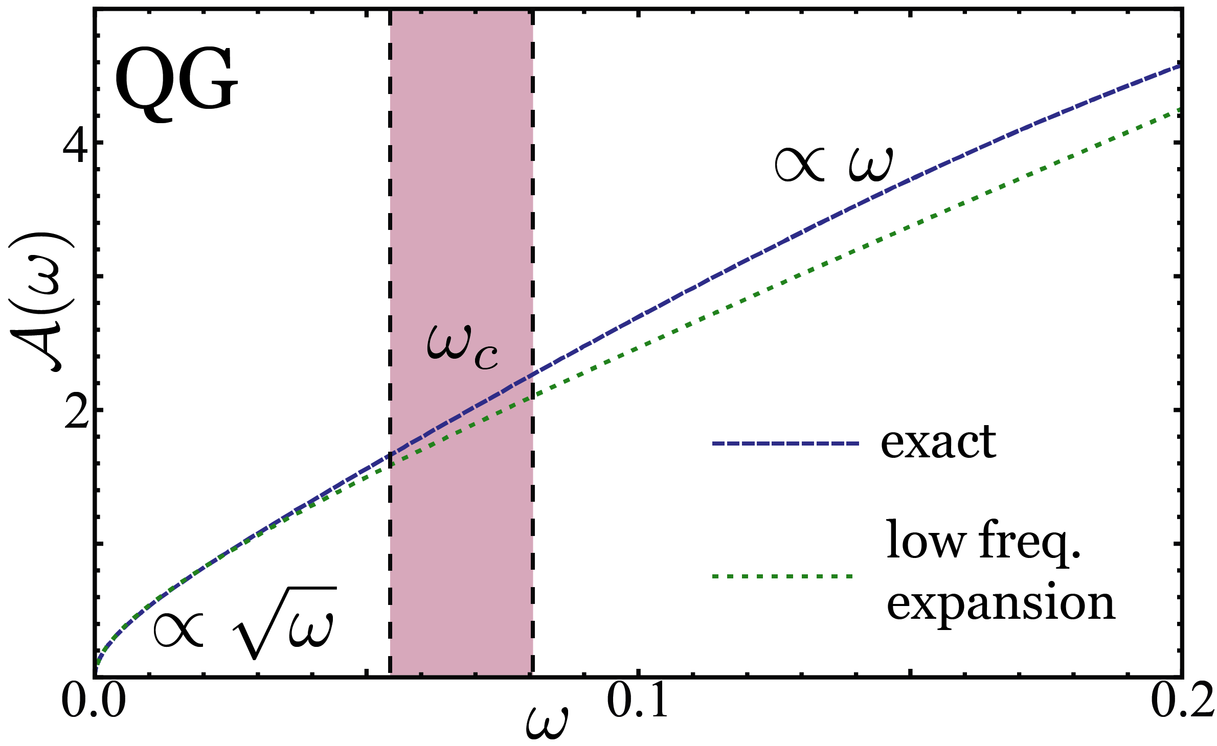
Figure 8: Spectral density $\mathcal{A}(\omega)=i\left(Q^{R}(\omega)-Q^{A}(\omega)\right)$ of the atoms in the glass phase for parameters ${K=0.01,\omega_{z}=2}$ and varying photon parameters $\omega_{p},\kappa$. For frequencies below the crossover ${\omega<\omega_{c}}$, $\mathcal{A}\sim\sqrt{\omega}$ is overdamped, corresponding to Eq. (211), while it recovers the typical thermal glass behavior $\mathcal{A}\sim\omega$ at intermediate frequencies ${\omega>\omega_{c}}$. Figure copied from Ref. Buchhold et al. (2013). (Copyright (2013) by The American Physical Society)

In the presence of dissipation, a photon that is emitted from an atom can either be absorbed by another atom, leading to an effective atom-atom interaction, which is infinite range in space, or decay from the cavity. The latter happens on a characteristic time scale $\tau_{p}=1/\kappa$, which is as well the time scale for which atoms can interact with each other by exchanging a photon before the photon decays. As a consequence, the photon decay reduces the effective range of the atom-atom interaction in time and reduces the strength of frustration in the system. Close to the glass transition and in the glass phase, this leads to the emergence of a crossover scale $\omega_{c}=\tau_{c}^{-1}$, above which the spectral properties of the system correspond exactly to a zero temperature spin glass. Below this frequency, the spectrum reveals the breaking of time reversal symmetry by the dissipation and formally corresponds to the dynamical universality class of dissipative quantum glasses, other examples of which are spin glasses coupled to an ohmic bath  Cugliandolo and Lozano (1999); Cugliandolo et al. (2002, 2004) or a bath of metallic electrons Read et al. (1995); Müller et al. (2012). The crossover frequency is

$$\omega_{\text{c}}=\kappa\left(\frac{\omega_{p}^{2}+\tfrac{1}{2}\kappa^{2}}{\omega_{p}^{2}+\kappa^{2}}+\frac{\left(\omega_{p}^{2}+\kappa^{2}\right)^{2}}{2\sqrt{K}\omega_{z}^{2}}\right)^{-1}.$$ (209)

and the modifications of the spectrum below this scale are due to the damping introduced by the Markovian bath. On the normal or disordered side of the phase diagram, the corresponding low frequency propagator is

$$Q^{R}_{n}(\omega)=Z\left((\omega+i\gamma)^{2}-\alpha^{2}\right)^{-1},$$ (210)

describing the Ising spins as damped harmonic oscillators with decay rate $\gamma>0$ and frequency $\alpha$, with the physical meaning of an inverse lifetime and energy gap of the atomic excitations. When the glass transition is approached, the gap, the inverse lifetime and the residue $Z$ scale to zero simultaneously and the atomic response in the glass phase

$$Q^{R}_{g}=\bar{Z}\left(\omega^{2}+\bar{\gamma}|\omega|\right)^{-\frac{1}{2}}$$ (211)

is non-analytic and can no longer be interpreted as a harmonic oscillator. The broken time reversal invariance manifests itself in both parameters $\gamma,\bar{\gamma}\neq 0$ being non-zero, which modifies the low frequency dynamics in the entire glass phase towards a dissipative quantum glass. This is for instance expressed by a spectral density, which features an anomalous square root behavior $\mathcal{A}(\omega)=-2\mbox{Im}(Q^{R}(\omega))\sim\sqrt{|\omega|}$ for small frequencies and therefore has a non-analytic response at zero frequency, see Fig. 8. The latter leads to a characteristic algebraic decay of the photon correlation function, as discussed below. The universality class of the present dissipative quantum glass transition is determined by the critical exponents at the transition, which describe the scaling of the parameters $\alpha,\gamma,Z$ as a function of $\delta=|K-K_{c}|$. It is summarized in the equations

$$\begin{array}[]{ccrl}\alpha_{\delta}&=&\frac{\sqrt{2}(\omega_{p}^{2}+\kappa^{2})}{8\sqrt{K^{3}}\kappa}&\left|\frac{\delta}{\log(\delta)}\right|^{\frac{3}{2}}\\ \gamma_{\delta}&=&\tfrac{\omega_{p}^{2}+\kappa^{2}}{16K^{2}\kappa}&\left|\frac{\delta}{\log(\delta)}\right|^{2}\\ Z_{\delta}&=&\tfrac{\omega_{p}(\omega_{p}^{2}+\kappa^{2})}{8\sqrt{K^{5}}\kappa^{2}}&\left|\frac{\delta}{\log(\delta)}\right|^{3}\end{array},$$ (215)

which show the typical logarithmic correction to scaling at a quantum glass transition and identify the critical exponents. Indicated by the scaling behavior, dissipative and coherent dynamics rival each other when approaching the transition, separating this glass transition from equilibrium transitions and the previously discussed Dicke transition, which are either fully coherent (quantum) with $\gamma=0$ or fully dissipative (classical) with $\alpha=0$ sufficiently close to the transition. The present glass transition has therefore no counterpart in static equilibrium physics and is termed dissipative quantum glass transition. Similar behavior is present in system bath settings in equilibrium, where the bath however not only imprints a finite temperature to the system but as well modifies its spectral properties  Cugliandolo et al. (2002); Cugliandolo and Lozano (1999); Müller et al. (2012). What these situations share in common is that the effective theory, after elimination of the bath variables, obeys no time reversal symmetry, which ensures the same asymptotic universal behavior as in the case of the Markovian photon loss in the present system.

III.2.3 Thermalization of photons and atoms in the glass phase

As typical for many open quantum systems (for exceptions, see the discussion in Sec. IV), the statistical properties of the excitations are described by a low energy effective temperature (LET) and a corresponding thermal distribution of the excitations. However, as has been found for the single mode Dicke model in the normal as well as in the superradiant phase, the LET for the photonic and the atomic subsystem did not coincide, i.e., the subsystems have not thermalized but are held at different temperatures corresponding to their individual coupling to a bath Dalla Torre et al. (2013). This dramatically changes in the present system with multiple photon modes. As frustration is increased by driving the variance $K$ towards the critical value $K_{c}$, atoms and photons begin to thermalize towards the same, shared LET. The distribution function $F$ of photonic or atomic modes is obtained by solving the fluctuation dissipation relation

$$Q^{K}(\omega)=Q^{R}(\omega)F_{\mbox{\tiny at}}(\omega)-F_{\mbox{\tiny at}}(\omega)Q^{A}(\omega)$$ (216)

for the atomic Green’s functions. It leads to an atomic LET

$$T_{\text{eff}}=\frac{\omega_{p}^{2}+\kappa^{2}}{4\omega_{p}}$$ (217)

in the glass phase, which coincides with the photonic LET Buchhold et al. (2013). The thermalization of the two subsystems is a consequence of the disorder induced effective long range interactions, which redistribute energy between the different modes and enable equilibration even in the presence of the Markovian dissipation in the photon sector. In the paramagnetic phase, the distribution functions of atoms and photons are identical for frequencies $\omega>\alpha$ larger than the gap, but deviate from each other for lower frequencies. The elementary excitations above this frequency are strongly correlated and can not be seen as weakly dressed photons or atoms. As a consequence, the observables in the critical glass phase are dominated by the universal low energy behavior of the glass propagator (211) and thermal statistics of the excitations.

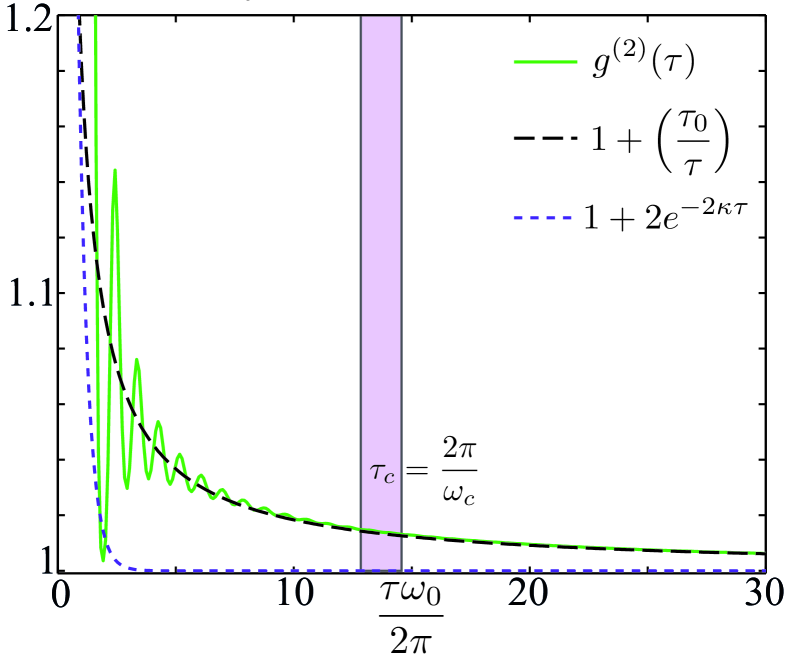
Figure 9: Algebraic decay of the photon four point correlation function $g^{(2)}(\tau)=\langle a^{\dagger}(0)a^{\dagger}(\tau)a(\tau)a(0)\rangle/n^{2}$ at long times, for parameters $\omega_{p}=1,\kappa=0.4,\omega_{z}=6,K=0.16$, see also Ref. Buchhold et al. (2013). The algebraic decay sets in at the inverse crossover frequency $\omega_{c}$, given by Eq. (209). The corresponding exponential decay of $g^{(2)}$ in the normal phase is plotted for comparison. Figure copied from Ref. Buchhold et al. (2013). (Copyright (2013) by The American Physical Society)

The strong light-matter interactions not only lead to thermalization of the atomic and photonic subsystems, they also feature a complete imprint of the glass dynamics of the atoms onto the cavity photons. This results in universal spectral properties of the photonic response, as has been shown in Ref. Buchhold et al. (2013), and concerns a complete locking of both subsystem’s low energy response properties. The photons form a photon glass state, which features a large, incoherent population of photon modes, signaled by a finite Edwards-Anderson parameter in the photon correlation function

$$G^{K}_{\mbox{\tiny ph}}(\omega)=4\pi\delta(\omega)\tilde{q}_{\mbox{\tiny EA}}+G^{K}_{\mbox{\tiny reg}}(\omega),$$ (218)

which shows the same scaling behavior as the atomic Edwards-Anderson parameter close to the glass transition $\tilde{q}_{\mbox{\tiny EA}}\sim q_{\mbox{\tiny EA}}$. A finite $\tilde{q}_{\mbox{\tiny EA}}$ implies long temporal memory in photon autocorrelation functions and an extensive number of photons permanently occupying a continuum of high energy modes. The latter is revealed by an algebraic decay of the system’s correlation functions, as for instance for the four point (or $g^{(2)}$) correlation function, which is shown in Fig. 9.

The photon response and correlation functions are easily accessible via cavity photon output measurements, and therefore represent the natural observables for the detection of the glass dynamics in cavity QED experiments. In fact, in Ref. Buchhold et al. (2013), it has been demonstrated that a complete characterization of the glass phase can be performed by different but standard photon output measurements, such as homodyne detection and intensity correlation measurements. Formally, the photon Green’s functions can be obtained from the Keldysh action formalism by introducing source fields $\mu_{\alpha\alpha^{\prime}}$ in the microscopic action, which couple to the photon variables. After integrating out the photon variables in the action, the photon Green’s functions are then obtained via functional derivatives with respect to these source fields. This standard field theory technique relates the photon Green’s functions to the solution for the atomic response and correlation functions Buchhold et al. (2013).

III.2.4 Quenched and Markovian bath coupling in the Keldysh formalism

The Keldysh path integral formalism represents a theoretical approach which incorporates in a very straightforward way the coupling of the system to a non-thermal bath. Here we compare quenched disorder and Markovian baths in more detail. As shown above in the present section, the coupling of the system variables to quenched disorder, realized by the variables $J_{lm}$, is equivalent to the coupling to a bath with infinite correlation time,

$$\langle J_{lm}(t)J_{l^{\prime}m^{\prime}}(t^{\prime})\rangle=\frac{K}{N}(\delta_{ll^{\prime}}\delta_{mm^{\prime}}+\delta_{lm^{\prime}}\delta_{ml^{\prime}}).$$ (219)

This represents the opposite limit of a Markovian bath, which has a typical correlation time that is much shorter than the system correlation time. As a consequence, at each single system-bath interaction event, the Markovian bath immediately equilibrates and looses all its memory on the interaction. On the other hand, the quenched bath equilibrates infinitely slowly and keeps memory on each single system-bath interaction. As a consequence, it introduces effective temporally long range interactions between the system variables. These tend to slow down the system, pronouncing its $\omega=0$ correlations as expressed by the Edwards-Anderson parameter.

In an equilibrium formalism, disordered systems have to be dealt with a computationally demanding replica method Ye et al. (1993); Read et al. (1995), which is furthermore physically far less transparent than the Keldysh formalism, which thus represents a convenient approach to disordered systems. In open quantum systems, where disorder, i.e., the coupling to a quenched bath, comes together with the dissipation introduced by a Markovian bath, both types of bath couplings compete with each other, leading in the present glassy system to strongly modified spectral properties, which mirror the effect of the Markovian bath by a crossover from non-equilibrium to equilibrium scaling behavior.

IV Non-equilibrium stationary states: bosonic models

Recent years have seen tremendous progress in experiments on exciton-polaritons in semiconductor microcavities (for reviews see, e.g., Refs. Carusotto and Ciuti (2013); Byrnes et al. (2014)), making these systems the prime candidates for studying condensation phenomena under non-equilibrium conditions. As we have already mentioned in Sec. I.3.2, the fundamental difference from conventional condensates is due to the finite life-time of exciton-polaritons, which makes continuous driving necessary to maintain a steady population.

What makes these systems genuinely driven-dissipative, is that they are coupled to several baths, or to time-dependent driving fields, with which they exchange particles and energy. In the case of exciton-polaritons, which are hybrid quasiparticles composed of a Wannier-Mott exciton and a photon, the photonic component can leak out through the mirrors forming the cavity. Thus, the electromagnetic vacuum outside the cavity serves as a reservoir into which particles are lost. These losses have to be compensated by laser driving. In many experiments, the driving laser is far blue-detuned from the bottom of the lower polariton band, and thus coherently creates high-energy excitations. During the relaxation of the latter, which is caused by phonon-polariton and stimulated polariton-polariton scattering, coherence is quickly lost. In other words, lower polaritons can be regarded as being pumped not directly by the laser but rather by a reservoir of high energy excitons. Several approaches have been used to model this effectively incoherent pumping mechanism Wouters and Carusotto (2007a); Szymańska et al. (2006, 2007). In this context, the description of a driven-dissipative condensate introduced in Sec. II.2.2 might be considered as a toy model, which hides all the microscopic details associated with coherent excitation and subsequent relaxation of high energy excitons in the coupling of the system to several independent baths.

In the following, we review recent investigations of the universal long-wavelength scaling properties of driven-dissipative condensates Sieberer et al. (2013, 2014); Altman et al. (2015); He et al. (2015); Gladilin et al. (2014); Ji et al. (2015). Then, the precise details of the chosen model cease to matter: according to the power-counting arguments given in Sec. II.3, for any choice of a microscopic model the effective long-wavelength description is given by the semiclassical Langevin equation for the condensate field (80). In fact, the latter can be derived in the spirit of Ginzburg-Landau theory for continuous phase transitions Lifshitz and Pitaevskii (1980) by writing down the most general equation that is compatible with the symmetries of the problem. The reasoning behind such an approach is that the universal properties are fully determined by the spatial dimensionality and symmetries of a physical system Amit and Martin-Mayor (2005); Zinn-Justin (2002); Goldenfeld (1992).

A comparison in terms of symmetries of systems exhibiting driven-dissipative Bose-Einstein condensation with systems in thermal equilibrium can be given most conveniently on the basis of the semiclassical limit of Sec. II.3: indeed, the equation of motion (80) for the classical field takes the form of the Langevin equations that are used to model universal dynamics in thermal equilibrium phenomenologically Hohenberg and Halperin (1977). Structurally, equation (80) is similar to model A for a non-conserved order parameter, with the additional inclusion of reversible mode couplings De Dominicis et al. (1975). However, the equilibrium symmetry discussed in Sec. II.4.1, which is present in all models of Ref. Hohenberg and Halperin (1977), is violated in driven-dissipative systems. This violation is due to pumping and loss terms, which moreover lead to the absence of particle number conservation. The latter typically is associated with the symmetry under quantum phase rotations (see Sec. II.4.4). This is another crucial difference to Bose-Einstein condensation in equilibrium: there, particle number conservation entails the existence of a slow dynamical mode that modifies the universal properties, and is taken into account in model F of Ref. Hohenberg and Halperin (1977). To summarize, driven-dissipative condensation differs from Bose-Einstein condensation in equilibrium by the absence of the equilibrium symmetry and the symmetry under quantum phase rotations. This difference lies at the heart of the novel universal behavior out of equilibrium discussed in the following.

In Sec. II.2.2, we analyzed driven-dissipative condensates within mean-field theory, disregarding fluctuations around the homogeneous condensate mode. However, in order to access universal aspects such as the behavior of correlations of the condensate field at large distances or dynamical critical phenomena at the condensation transition, one has to carefully include the effect of fluctuations. This can be done gradually — first integrating out short-scale fluctuations and moving on to account for fluctuations on larger and larger scales — by means of RG methods, such as the FRG discussed in Sec. II.5. Then, an intriguing question is, whether the non-equilibrium nature of driven-dissipative condensates at the microscopic scale becomes more or less pronounced under renormalization. In the former case, effective equilibrium is established at large scales, while in the latter case, the universal physics is expected to be profoundly different from its equilibrium counterpart. Which of these scenarios is realized depends crucially on the spatial dimensionality of the system: in 3D the long-wavelength regime is effectively thermal, whereas in one- and two-dimensional systems the deviation from equilibrium is relevant in the RG sense, and these systems are governed by strongly non-equilibrium RG fixed points.

To see how this comes about, we require a quantitative measure for the deviation from equilibrium conditions in a driven-dissipative condensate. In Sec. II.4.1 we discussed that thermal equilibrium requires the ratios of coherent to corresponding dissipative couplings to take a common value. This is illustrated in Fig. 6 and formalized in Eq. (101). In turn, it implies that any deviation $K_{c}/K_{d}\neq u_{c}/u_{d}$ in the values of these ratios directly indicates a deviation from equilibrium conditions. Hence, the quantity $\lambda$ defined by Altman et al. (2015)

$$\lambda=-2K_{c}\left(1-\frac{K_{d}u_{c}}{K_{c}u_{d}}\right)$$ (220)

can serve as a quantitative measure for the departure from thermal equilibrium. Note that $\lambda=0$ in equilibrium, and that $\lambda$ is well-defined also for $K_{d}=0$, which is the microscopic value of the diffusion constant $K_{d}$ in the model for driven-dissipative condensates introduced in Sec. II.2.2. It turns out to be most convenient to combine $\lambda$ with the quantities Altman et al. (2015)

$$D=K_{c}\left(\frac{K_{d}}{K_{c}}+\frac{u_{c}}{u_{d}}\right),\quad\Delta=\frac{\gamma}{2\rho_{0}}\left(1+\frac{u_{c}^{2}}{u_{d}^{2}}\right)$$ (221)

(see Sec. II.2.2 for the definition of the noise strength $\gamma$ and the mean-field condensate density $\rho_{0}$) to define the dimensionless non-equilibrium strength as Täuber (2014):

$$g=\Lambda_{0}^{d-2}\frac{\lambda^{2}\Delta}{D^{3}},$$ (222)

where $\Lambda_{0}$ is the UV momentum cutoff. Thus, the answer to the question of whether equilibrium vs. non-equilibrium universal behavior is realized in driven-dissipative condensates, is encoded in the RG flow of $g$.

In the condensed phase, the RG flow of $g$ is driven dominantly by fluctuations of the gapless Goldstone mode discussed in Sec. II.4.6, i.e., by fluctuations of the phase of the condensate field. The latter were shown Sivashinsky (1977); Kuramoto (1984); Grinstein et al. (1993, 1996) to be governed by the Kardar-Parisi-Zhang (KPZ) equation Kardar et al. (1986), in which $\lambda$ defined in Eq. (220) appears as the coefficient of the characteristic non-linear term, see Eq. (231). Below in Sec. IV.1, we present an alternative mapping of the long-wavelength condensate dynamics to the KPZ equation, starting from the Keldysh action in Eq. (73) and integrating out the gapped density mode within the Keldysh functional integral. As a consequence of the mapping to the KPZ equation, the RG flow of $g$ in $d$ spatial dimensions is at the one-loop level given by Täuber (2014)

$$\partial_{\ell}g=-\left(d-2\right)g+\frac{\left(2d-3\right)C_{d}}{2d}g^{2},$$ (223)

where $\ell=\ln(\Lambda/\Lambda_{0}),$ $\Lambda$ is the running momentum cutoff, and $C_{d}=2^{1-d}\pi^{-d/2}\Gamma(2-d/2)$ is a geometric factor. The key role that is played by spatial dimensionality becomes manifest in the canonical scaling of $g$, which is encoded in the first term on the RHS of the flow equation: to wit, $g$ is relevant in 1D where $d-2<0$, marginal in 2D, and irrelevant in 3D since then $d-2>0$. In 2D, the loop correction — the second term on the RHS of Eq. (223) — is positive, making $g$ marginally-relevant. This has far-reaching consequences for a driven-dissipative condensate in which the microscopic value of $g$ is small, i.e., which is close to equilibrium: upon increasing the scale at which the system is observed, the non-equilibrium nature is more pronounced in one- and two-dimensional systems, whereas effective equilibrium is established on large scales in three-dimensional systems. In 1D the canonical scaling towards strong coupling is balanced at an attractive strong-coupling fixed point (SCFP) $g_{*}$ by the loop correction. This term vanishes at $d=3/2,$ and for $d>3/2$ the one-loop equation does not have a stable SCFP, which, however, is recovered in a non-perturbative FRG approach Canet et al. (2010, 2011b, 2012). The RG flow of $g$ that is found within this approach is illustrated qualitatively in Fig. 10, which shows that also in 2D the flow is out of the shaded close-to-equilibrium regime with $g<1$, and towards a strong-coupling, non-equilibrium fixed point. The situation is quite different in 3D: in this case, if the microscopic value of $g$ is small, at large scales an effective equilibrium with a renormalized value $g\to 0$ is reached. However, for $d>2$, there exists a critical line of unstable fixed points $g_{c}$, separating the basins of attraction of the equilibrium and non-equilibrium fixed points, for $g<g_{c}$ and $g>g_{c}$ respectively. Thus, in addition to the effective equilibrium phase, a true non-equilibrium phase may be reached in systems that are far from equilibrium even at the microscopic level also in 3D Fisher and Grinstein (1992). The properties of this phase have not been explored so far.

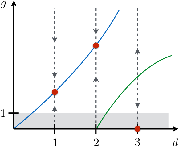
Figure 10: Equilibrium vs. non-equilibrium phase diagram for driven-dissipative condensates (cf. Ref. Canet et al. (2010)). The line $g=1$, where $g$ is defined in Eq. (222) and measures the deviation from equilibrium conditions, separates the close-to-equilibrium regime for $g<1$ from the strong-coupling, far-from-equilibrium regime at $g>1$. Red dots indicate the fixed-point values of $g$ that are reached if the RG flow is initialized in the close-to-equilibrium regime. In dimensions one and two, the equilibrium fixed point at $g=0$ is unstable, and the RG flow along the dashed lines is directed towards the blue line of strong-coupling fixed points. Thus, a system that is microscopically close to equilibrium will exhibit strongly non-equilibrium behavior at large scales. On the other hand, in three spatial dimensions, an initially small value of $g$ is diminished under renormalization, and the universal large-scale behavior is governed by the effective equilibrium fixed point at $g=0$. The green line indicates the existence of a critical value $g_{c}$ in $d>2$, corresponding to a transition between the effective equilibrium phase and a true non-equilibrium phase that is realized for large microscopic values $g>g_{c}$.

The rest of this section is organized as follows: in Sec. IV.2, we review the dynamical critical behavior at the driven-dissipative condensation transition in 3D Sieberer et al. (2013, 2014); Täuber and Diehl (2014), which, according to the above discussion, is governed by an effective equilibrium fixed point. Signatures of the non-equilibrium nature of the microscopic model are present in the asymptotic fade-out of the deviation from equilibrium at large scales. In contrast, the universal scaling behavior of driven-dissipative condensates in both 2D Altman et al. (2015) and 1D Gladilin et al. (2014); Ji et al. (2015); He et al. (2015) is quite distinct from the equilibrium case and governed by the SCFP of the KPZ equation. We review the resultant physical picture in Secs. IV.3 and IV.4, respectively.

IV.1 Density-phase representation of the Keldysh action

Especially in reduced dimensions, at large scales the properties of condensates are vitally influenced by fluctuations of the Goldstone mode. To name an example, in 2D, both in Mermin and Wagner (1966) and out of equilibrium Altman et al. (2015) these fluctuations lead to a suppression of long range correlations. In Ref. Altman et al. (2015), an effective long-wavelength description of a driven-dissipative condensate with the condensate phase as the single dominant gapless degree of freedom (cf. Sec. II.4.6) has been formulated starting from the Langevin equation (80) for the complex order parameter. Here we present an alternative and direct derivation within the Keldysh functional integral formalism Kamenev (2011); Altland and Simons (2010). It is based on the Keldysh action in terms of which the microscopic theory of a bosonic many-body system with particle loss and gain is formulated in Sec. II.2.2. This differs from the derivation presented in Altman et al. (2015), which was based on the detour over the Langevin equation (80) that effectively captures the physics on a mesoscopic scale (cf. Fig. 5 and the discussion in Sec. II.3). On this level, amplitude fluctuations can be eliminated leading to the KPZ equation for the phase. In this sense, we establish here a closer link between microscopic and mesoscopic theories, which is both appealing from a theoretical point of view and brings about a number of technical advantages. For example, physical observables are usually represented by quantum mechanical operators or equivalently in terms of fields in a Keldysh functional integral description of the microscopic theory; here our approach comes in handy as it yields the effective long-wavelength form of generating functionals for expectation values and correlation functions of these observables which can then be evaluated further utilizing established approximation strategies.

Apart from specific applications, the derivation of the action for the Goldstone mode presented here deepens our understanding of general properties of the Keldysh formalism with regard to phase rotation symmetries. The crucial point is, that classical phase rotations introduced in Sec. II.4.4 are a symmetry of the Keldysh action both in a closed system and in the presence of terms that describe incoherent pumping and losses, and as we have seen in Sec. II.4.6, the spontaneous breaking of this symmetry is sufficient to ensure the appearance of a Goldstone mode that corresponds to fluctuations of the phase of the order parameter Wouters and Carusotto (2006); Szymańska et al. (2006); Wouters and Carusotto (2007a, b). In the basis of classical and quantum fields $\phi_{c,q}$ such phase rotations become $\phi_{c,q}\mapsto\phi_{c,q}e^{i\alpha}$, showing that the Goldstone mode corresponds to joint phase fluctuations of both the classical and the quantum fields. Therefore, in order to derive the action for the Goldstone boson we represent the fields in the form

$$\phi_{c}=\sqrt{\rho}e^{i\theta},\quad\phi_{q}=\zeta e^{i\theta},$$ (224)

where the density $\rho$ is real whereas $\zeta$ is a complex variable.

The low-energy effective action for the Goldstone boson $\theta$ in a driven-dissipative system can be derived by integrating out fluctuations of the density $\rho$ in Eq. (224) in the Keldysh partition function with action $S$ given by Eq. (73),

$$Z=\int\mathscr{D}[\phi_{c},\phi_{c}^{*},\phi_{q},\phi_{q}^{*}]e^{iS}=\int\mathscr{D}[\rho,\theta,\zeta,\zeta^{*}]e^{iS}.$$ (225)

The equality of the integrals over complex classical and quantum fields and the variables introduced in the transformation Eq. (224) follows from the fact that this transformation leaves the integration measure invariant, i.e., we have $\mathscr{D}[\phi_{c},\phi_{c}^{*},\phi_{q},\phi_{q}^{*}]=\mathscr{D}[\rho,\theta,\zeta,\zeta^{*}]$. Note that this would not be the case if instead of the density we introduced the amplitude of $\phi_{c}$ as a degree of freedom. Our goal is then to treat the integrals over $\rho$ and $\zeta$ in Eq. (225) in a saddle-point approximation, which, as we show below, is justified since fluctuations of the density are gapped in the ordered phase with $r_{d}<0$ and hence expected to be small. The first step is thus to find the saddle point, i.e., the solutions to the classical field equations (cf. Eqs. (74))

$$\frac{\delta S}{\delta\rho}=0,\quad\frac{\delta S}{\delta\zeta}=0.$$ (226)

For $r_{d}<0$, we recover the mean-field solution of Sec. II.2.2, given by $\rho=\rho_{0}=-r_{d}/u_{d}=-r_{c}/u_{c}$ (note that the last equality can always be satisfied by performing a gauge transformation to adjust the value of $r_{c}$ as described in Sec. II.2.2) and $\zeta=0$. We proceed to expand the action Eq. (73) to second order in fluctuations of $\rho$ and $\zeta$ around the saddle point. Note that the quantum vertex in the action Eq. (73) that is cubic in the quantum fields does not contribute at this order. Denoting the density fluctuations as $\pi=\rho-\rho_{0}$ we find

$$S=2\int_{t,\mathbf{x}}\left(\sqrt{\rho_{0}}\left\{-\zeta_{1}\left[\partial_{t}\theta+K_{c}\left(\nabla\theta\right)^{2}\right]+K_{c}\zeta_{2}\nabla^{2}\theta\right.\right.\\ \left.\left.\vphantom{\left(\nabla\theta\right)^{2}}-\left(u_{c}\zeta_{1}-u_{d}\zeta_{2}\right)\pi\right\}+i\left(\gamma+2u_{d}\rho_{0}\right)\left\lvert\zeta\right\rvert^{2}\right),$$ (227)

where $\zeta_{1}$ and $\zeta_{2}$ are, respectively, real and imaginary parts of $\zeta$. Here, of all terms involving the products of fluctuations $\zeta_{1}\pi$ and $\zeta_{2}\pi$ we only keep the dominant ones in the long-wavelength limit, i.e., we neglect contributions containing temporal derivatives $\zeta_{2}\partial_{t}\pi,\zeta_{1}\pi\partial_{t}\theta$, and spatial derivatives $\zeta_{1}\nabla^{2}\pi,\zeta_{2}\nabla\pi\cdot\nabla\theta,$ and $\zeta_{1}\pi\left(\nabla\theta\right)^{2}$ which are both small as compared to the mass-like contributions $u_{c}\zeta_{1}\pi$ and $u_{d}\zeta_{2}\pi$ in Eq. (227) for the Goldstone mode $\theta$, in the regime $\omega\to 0$ for $\mathbf{q}\to 0$. Note that terms of higher order in $\pi$ and $\zeta$ are contained in the original action Eq. (73) both in contributions involving derivatives and in the coherent and dissipative vertices. The validity of the saddle-point approximation, therefore, is restricted to the low-frequency and low-momentum sector in a weakly interacting system.

The action (227) resulting from this expansion is linear in $\pi$ and hence integration over this variable is trivial and yields a $\delta$-functional, which in turn facilitates integration over the imaginary part $\zeta_{2}$ of $\zeta$,

$$Z=\int\mathscr{D}[\theta,\zeta_{1},\zeta_{2}]\,\delta[u_{c}\zeta_{1}-u_{d}\zeta_{2}]e^{iS^{\prime}}=\int\mathscr{D}[\theta,\tilde{\theta}]\,e^{iS_{\mathrm{KPZ}}},$$ (228)

where at each step a normalization factor is implicitly included in the integration measure, ensuring $Z=1$ Kamenev (2011); Altland and Simons (2010). In the last equality we replaced $\zeta_{1}$ by the KPZ response field $\tilde{\theta}=i2\sqrt{\rho_{0}}\zeta_{1}$, and the KPZ action $S_{\mathrm{KPZ}}$ is given by Täuber (2014); Kamenev (2011)

$$S_{\mathrm{KPZ}}=\int_{t,\mathbf{x}}\tilde{\theta}\left[\partial_{t}\theta-D\nabla^{2}\theta-\frac{\lambda}{2}\left(\nabla\theta\right)^{2}-\Delta\tilde{\theta}\right],$$ (229)

where the diffusion constant, non-linear coupling, and noise strength, respectively, are expressed in terms of the microscopic parameters in the original action Eq. (73) as

$$D=K_{c}\frac{u_{c}}{u_{d}},\quad\lambda=-2K_{c},\quad\Delta=\frac{\gamma+2u_{d}\rho_{0}}{2\rho_{0}}\left(1+\frac{u_{c}^{2}}{u_{d}^{2}}\right).$$ (230)

Along the lines of the derivation of the Langevin equation (80) from the action in the semiclassical limit in Eq. (79), the KPZ action can be seen to be equivalent to the KPZ equation, which reads

$$\partial_{t}\theta=D\nabla^{2}\theta+\frac{\lambda}{2}\left(\nabla\theta\right)^{2}+\eta,$$ (231)

where the stochastic noise $\eta$ has zero mean, $\langle\eta(t,\mathbf{x})\rangle=0$, and is Gaussian with second moment $\langle\eta(t,\mathbf{x})\eta(t^{\prime},\mathbf{x}^{\prime})\rangle=2\Delta\delta(t-t^{\prime})\delta(\mathbf{x}-\mathbf{x}^{\prime})$. Originally Halpin-Healy and Zhang (1995); Kardar et al. (1986), Eq. (231) was suggested by Kardar, Parisi, and Zhang as a model to describe the growth of a surface, e.g., due to the random deposition of atoms. In this context, $h=\theta$ is the height of the surface, and the origin of the non-linear term is purely geometric Kardar et al. (1986): the growth is assumed to occur in a direction that is locally normal to the surface and at a rate $ds/dt=\lambda$; If an increment $ds=\lambda dt$ is added along the normal, the corresponding change of the surface height is

$$dh=\sqrt{\left(\lambda dt\right)^{2}+\left(\lambda dt\nabla h\right)^{2}}\approx\left[\lambda+\frac{\lambda}{2}\left(\nabla h\right)^{2}\right]dt.$$ (232)

Removing from $dh/dt$ the average deposition rate $\lambda$ by a transformation to a co-moving frame, $h(t,\mathbf{x})\mapsto h(t,\mathbf{x})+\lambda t$, and adding a term $D\nabla^{2}h$ that describes surface tension, we obtain the (deterministic part of the) growth equation (231). Intuitively, it seems clear that the growth of a surface represents a genuine non-equilibrium process. More formally, this can be seen by noting that the non-linear term in the KPZ equation does in general not satisfy a potential condition Täuber (2014).

As pointed out above, an alternative derivation of the KPZ equation (231) as the effective long-wavelength description of driven-dissipative condensates starts from the Langevin equation (80) Altman et al. (2015). Then, the coefficients in the KPZ equation are slightly different, and they are given by Eqs. (220) and (221) instead of Eq. (230). To be specific, the differences are (i) the absence in Eq. (221) of the tree-level shift $\propto u_{d}\rho_{0}$ of the noise strength $\Delta$ in Eq. (230), and (ii) the absence in Eq. (230) of the terms proportional to $K_{d}$ in Eqs. (220) and (221). (i) is due to the fact that in the Langevin equation (80), which is valid in the semiclassical limit (see Sec. II.3), the quantum vertex that is proportional to $\phi_{c}^{*}\phi_{c}\phi_{q}^{*}\phi_{q}$ in the action in Eq. (73) is neglected. (ii) results from the absence of the diffusion term $K_{d}$ in the microscopic model (73); on the other hand, in the Langevin equation (80) this term is included, as it is generated by integrating out fluctuations with wavelengths below the mesoscopic scale on which the Langevin equation is valid (cf. Fig. 5).

Starting from the effective long-wavelength description of the condensate dynamics derived in this section, the universal scaling properties can be obtained from an RG analysis. For the KPZ equation, this procedure, which leads at lowest order in a perturbative expansion in $\lambda$ to the one-loop flow equation (223), is described, e.g., in Refs. Täuber (2014); Kamenev (2011).

For completeness, we note that in the absence of drive and dissipation, i.e., for $K_{d}=r_{d}=u_{d}=0$, an analogous derivation for a weakly interacting Bose gas in thermal equilibrium leads to an effective action for the phase alone that is given by

$$S=\int_{t,\mathbf{x}}\tilde{\theta}\left(\partial_{t}^{2}-c^{2}\nabla^{2}\right)\theta,$$ (233)

where $c=\sqrt{2K_{c}u_{c}\rho_{0}}$ is the speed of sound, and describes the dissipationless propagation of sound waves with linear dispersion $\omega=cq.$ To actually describe thermal equilibrium, this action has to be supplemented by infinitesimal regularization terms, discussed at the end of Sec. II.2.1.

Finally, let us comment on the relation of the approach presented here to a Bogoliubov expansion in fluctuations of the complex fields around the mean field average values, $\delta\phi_{c}=\phi_{c}-\sqrt{\rho_{0}}$ and $\delta\phi_{q}=\phi_{q}$. The latter can be recovered formally by expanding the transformation Eq. (224) around the arbitrarily chosen value $\theta=0$, which yields

$$\phi_{c}=\sqrt{\rho_{0}}+\frac{\pi}{2\sqrt{\rho_{0}}}+i\sqrt{\rho_{0}}\theta,\quad\phi_{q}=\zeta,$$ (234)

and interpreting $\pi$ and $\theta$ as the real and imaginary parts of $\delta\phi_{c}$. In the KPZ action in Eq. (229), such an expansion in $\theta$ would amount to neglecting the non-linearity. Without the non-linearity, however, the KPZ action describes a free field coupled to a thermal bath. In other words, by performing a Bogoliubov approximation the non-equilibrium character that is intrinsic to the microscopic model with action (73) is lost in the long-wavelength limit. Formally, this failure is due to the fact that the saddle-point approximation is not valid for low-momentum modes in the Goldstone direction since they are not gapped.

IV.2 Critical dynamics in 3D

In three spatial dimensions, the deviation from thermodynamic equilibrium conditions, which is quantified by the value of $g$ defined in Eq. (222), is irrelevant in the RG sense (cf. Eq. (223)). Hence, at large scales, effective equilibrium is established. This immediately implies that the overall picture of Bose-Einstein condensation in thermal equilibrium in 3D remains valid also in the driven-dissipative context: in particular, the mean-field analysis of Sec. II.2.2, which predicts a continuous phase transition beyond which the classical phase rotation symmetry (cf. Sec. II.4.4) is spontaneously broken and off-diagonal long-range order is established, is modified quantitatively but not qualitatively once fluctuations around the mean-field condensate are taken into account. (Note, however, that in equilibrium the condensation transition is induced by lowering the temperature to a critical value, whereas driven-dissipative condensation is established by tuning the single-particle pump rate.) Yet, the non-equilibrium nature of the driven-dissipative system leaves its mark on the approach to the long-wavelength thermalized regime in a fully universal way.

An equilibrium system, fine-tuned to a critical point, beyond which spontaneous symmetry breaking occurs via a second order phase transition, exhibits universal behavior. This is witnessed in non-analyticities in the free energy, and in the long-range decay properties of correlation and response functions. The decay properties are then governed by power laws, freed from the generic exponential cutoff $\sim e^{-r/\xi}$ at large distances $r$ due to the divergent correlation length $\xi\to\infty$, defining the critical point. While the concept of a free energy is not meaningful in a non-equilibrium context, correlations and responses can be considered also in the latter case. Then, universality entails that the algebraic long-wavelength, long-time decay of any correlation or response function can be characterized in terms of a set of critical exponents, which do not depend on the microscopic details of the problem but rather on symmetries and dimensionality. The critical point is fully characterized by this set of critical exponents.

We emphasize a crucial difference between the critical behavior in strictly non-interacting theories described by quadratic Hamiltonians or quantum master equations, and the more generic — but also much more complex — case of interacting problems (for an example where a Gaussian fixed point is physically important, cf. Sec. III.1). The non-interacting critical theories are described by a so-called Gaussian fixed point of the RG flow, while the interacting ones are associated to a so-called Wilson-Fisher fixed point. The structural difference between these fixed points is reflected by the fact that the values of the critical exponents differ; in particular, at a Gaussian fixed point, all exponents are rational numbers, reflecting the validity of canonical power counting (cf. Sec. II.3), while one obtains non-trivial rational or non-rational numbers mirroring the importance of strong long-wavelength fluctuation corrections at a Wilson-Fisher fixed point. The latter is more stable than the Gaussian one (where, in fact, all couplings are relevant in the sense of the RG), and thus the physically relevant one even if interactions are small on the microscopic scale. This is intuitive, taking into account that critical behavior deals with the longest distances and timescales in a physical system.

The impact of fluctuations on the values of the critical exponents can be described quantitatively in the framework of the renormalization group, which provides a systematic way to deal with the intricate long-wavelength, low-momentum divergences caused by the divergent correlation length. The critical behavior of driven-dissipative systems in 3D was investigated in Sieberer et al. (2013, 2014) based on the functional renormalization group approach discussed in Sec. II.5, and in Täuber and Diehl (2014) using the field theoretic perturbative renormalization group Täuber (2014). These studies gave rise to the following picture of driven criticality:

The RG fixed point is purely dissipative (see Fig. 6 (c)), i.e., all complex couplings rotate to the imaginary axis. However, it is the approach to this fixed point that contains universal information, and this makes it possible to distinguish equilibrium from non-equilibrium critical behavior. The following key properties are identified:

(i) Asymptotic thermalization of correlation functions. — Both the static and dynamical critical exponents, governing, e.g., the asymptotic decay of the spatial and temporal first order coherence functions, are found to take the same values as in the corresponding equilibrium problem. This can be made plausible by the fact that the fixed point couplings indeed lie on a single ray in the complex plane — the imaginary axis. More formally, it is understood in terms of an emergent symmetry implying asymptotic emergence of detailed balance, or thermalization, at large spatial or temporal distances.

(ii) Universal decoherence. — The approach to the purely dissipative fixed point still hosts information on the underlying quantum dynamics. The fadeout of this coherent dynamics is described by a new critical exponent, which can be shown to be independent of the static and dynamical exponents, i.e., it does not relate to the latter by scaling relations. Moreover, it can be seen that no more independent exponents could possibly be found Sieberer et al. (2013); Täuber and Diehl (2014). This is because the maximum number of independent exponents is determined by the maxium number of independent microscopic mass scales Goldenfeld (1992), which are, in the quadratic part of the action (79), given by the real parameters $r_{c},r_{d},$ and $\gamma$. In addition, a coupling $f$ to an external source field, corresponding to a term $\int_{t,\mathbf{x}}f\left(j_{c}^{*}\phi_{q}+j_{q}^{*}\phi_{c}+\mathrm{c.c.}\right)$ in the action, has to be taken into account, leading in total to four independent parameters. No more independent scales can be added to the quadratic part of the action without violating the conditions of (Anti-)Hermiticity and conservation of probability as explained in Sec. II.2.1. Correspondingly, the set of four independent critical exponents (the correlation length exponent $\nu$, the anomalous dimension $\eta$, the dynamical critical exponent $z$, and new exponent) is maximal. Finally, the value of this exponent distinguishes equilibrium from non-equilibrium conditions. This can be understood from Fig. 6: the exponent describes the fadeout of coherent couplings, i.e., the approach to the imaginary axis, governed by a power law $\sim\Lambda^{-\eta_{r}}$, where $\eta_{r}$ is the new exponent. In the equilibrium case, all couplings rotate uniformly, giving rise to $\eta_{r}\approx-0.143$ within the FRG approach of Refs. Sieberer et al. (2013, 2014). In contrast, in the non-equilibrium case, the slowest approach to the real axis is given by $\eta_{r}\approx-0.101$. The value of the non-equilibrium exponent can also be determined analytically from the field theoretic perturbative renormalization group in a dimensional expansion, yielding the result (to two-loop order) Täuber and Diehl (2014)

$$\eta_{r}=-\frac{2\left(4-d\right)^{2}}{25}\ln\frac{4}{3}.$$ (235)

Specifying to $d=3$ dimensions, we obtain $\eta_{r}\approx-0.023$. The discrepancy between this value and the one obtained from the FRG stated above ($\eta_{r}\approx-0.101$) indicates that the two-loop computation underestimates fluctuation corrections in three dimensions. Moreover, (possibly significant) quantitative corrections to the values of critical exponents should also be expected from FRG calculations that go beyond the truncation used in Refs. Sieberer et al. (2013, 2014).

(iii) Observability. — The drive exponent manifests itself, for example, in the frequency and momentum resolved dynamical single particle response as probed in homodyne detection, see Ref. Sieberer et al. (2014) for details. It thus corresponds to a direct experimental observable, though its small value poses a challenge for experimental observation.

In summary, it is found that the correlation functions (both static and dynamic) thermalize, and show identical universal behavior to an equilibrium critical system with the same symmetries. However, the dynamical response functions contain universal information distinguishing equilibrium from non-equilibrium systems. The microscopic drive conditions are thus witnessed even at the largest macroscopic distances in a fully universal way.

In the following, we review how the results summarized above can be obtained from an open-system functional RG approach Sieberer et al. (2013, 2014). The basic ingredients of this method are discussed in Sec. II.5.

IV.2.1 Effective action for driven-dissipative condensation

The Wetterich equation (132) describes how the scale-dependent effective action $\Gamma_{\Lambda}$ evolves from the microscopic action $S$ at $\Lambda=\Lambda_{0}$ to the full effective action $\Gamma$ at $\Lambda\to 0$, as fluctuations with momenta larger than the cutoff $\Lambda$ are integrated out, and the latter is gradually lowered. It is an exact non-linear differential equation for the functional $\Gamma_{\Lambda}$. In the absence of an exact solution, suitable schemes to approximate the functional differential equation have to be found. For the analysis of critical behavior, progress can be made by choosing an ansatz for $\Gamma_{\Lambda}$ that has a similar structure as the microscopic action $S$ in Eq. (73). In this way, the effective action $\Gamma_{\Lambda}$ is parameterized in terms of the coupling constants appearing in the ansatz, and consequently, the functional differential equation for $\Gamma_{\Lambda}$ can be cast in the form of a set of ordinary differential equations for the couplings, as we describe in detail below.

Any such ansatz will contain only a finite number of couplings, and will hence truncate the most general structure of $\Gamma_{\Lambda}$. In other words, by choosing an ansatz of a particular form, one makes an approximation, and the question arises, which couplings should be included in the ansatz or truncation in order to obtain meaningful results. For the study of critical phenomena at a second order phase transition, the power counting scheme of Sec. II.3 provides a guideline: following the arguments given there, we choose a truncation which includes all couplings that are not irrelevant, and which therefore takes the form of the semiclassical action in Eq. (79):

$$\Gamma_{\Lambda}=\int_{t,\mathbf{x}}\left\{\bar{\phi}_{q}^{*}\left[\left(iZ^{*}\partial_{t}+\bar{K}^{*}\nabla^{2}\right)\bar{\phi}_{c}-\frac{\partial\bar{U}^{*}}{\partial\bar{\phi}_{c}^{*}}\right]+\mathrm{c.c.}+i\bar{\gamma}\bar{\phi}_{q}^{*}\bar{\phi}_{q}\right\}.$$ (236)

(Recall that the variables of the effective action are the field expectation values $\bar{\Phi}_{\nu},\nu=c,q$ defined in Eq. (37).) Here, in addition to the complex prefactor $\bar{K}=\bar{A}+i\bar{D}$ of the Laplacian, we are including a complex wave-function renormalization $Z=Z_{R}+iZ_{I}$. In the semiclassical limit, the homogeneous (i.e., not containing derivatives with respect to time or space) part of the action can be written in terms of an effective potential $\bar{U}$, which is a function of $\bar{\rho}_{c}=\bar{\phi}_{c}^{*}\bar{\phi}_{c}$. Due to the invariance of the microscopic action under classical phase rotations (cf. Sec. II.4.4), which is inherited by the effective action, only this combination of fields is allowed in the potential. The latter is given by

$$\bar{U}(\bar{\rho}_{c})=\frac{1}{2}\bar{u}_{2}\left(\bar{\rho}_{c}-\bar{\rho}_{0}\right)^{2}+\frac{1}{6}\bar{u}_{3}\left(\bar{\rho}_{c}-\bar{\rho}_{0}\right)^{3}.$$ (237)

Here, both the two-body and three-body couplings, $\bar{u}_{2}=\bar{\lambda}+i\bar{\kappa}$ and $\bar{u}_{3}=\bar{\lambda}_{3}+i\bar{\kappa}_{3}$, respectively, are complex. The three-body term is marginal according to power counting, and therefore included in the truncation. In the FRG, it is advantageous to approach the transition from the ordered phase. Then, the form of the effective potential in Eq. (237) corresponds to an expansion around the stationary condensate density $\bar{\rho}_{0}$. Indeed, this choice implies, that the field equations $\delta\Gamma_{\Lambda}/\delta\bar{\phi}_{c}^{*}=0,\delta\Gamma_{\Lambda}/\delta\bar{\phi}_{q}^{*}=0$ (Eqs. (40) in the absence of sources and evaluated with the scale-dependent effective action $\Gamma_{\Lambda}$) are solved by $\bar{\rho}_{c}=\bar{\rho}_{0}$ and $\bar{\phi}_{q}=0$ on all scales $\Lambda$.

In the truncation Eq. (236), all couplings — including the condensate density $\bar{\rho}_{0}$ — are scale dependent. As indicated above, by means of such an ansatz for the effective action $\Gamma_{\Lambda}$, the functional differential equation (132) can be rewritten as a set of ordinary differential equations for these running couplings, with initial conditions given by the microscopic action Eq. (79). This is achieved by applying projection prescriptions. In the following, we summarize this method for the problem at hand. For details we refer the reader to Ref. Sieberer et al. (2014).

IV.2.2 Non-equilibrium FRG flow equations

The main idea of a projection prescription on a specific coupling is to extract this coupling from the effective action $\Gamma_{\Lambda}$ by taking appropriate derivatives of the latter with respect to the fields and coordinates, and subsequently setting the fields to their stationary values $\bar{\phi}_{c}=\bar{\phi}_{0}=\sqrt{\bar{\rho}_{0}}$ and $\bar{\phi}_{q}=0$ (as noted in Sec. II.4.6, choosing $\bar{\phi}_{c}$ to be real does not lead to a loss of generality). Then, applying the very same projection description to the Wetterich equation (132) yields the flow equation for the corresponding coupling. For the actual evaluation of the resulting flow equations, it is convenient to introduce rescaled fields, which are related to the bare ones by absorbing the wave-function renormalization $Z$ in the quantum field:

$$\phi_{c}=\bar{\phi}_{c},\quad\phi_{q}=Z\bar{\phi}_{q}.$$ (238)

As a consequence of this transformation, and by rescaling all couplings appropriately, it is possible to obtain a reduced set of flow equations, from which $Z$ is eliminated. In a second step, the number of flow equations can be diminished further by introducing dimensionless renormalized variables, as detailed in Sec. IV.2.3 below.

We start by deriving flow equations for the non-linear couplings in the effective potential defined in Eq. (237). To see how one can project the Wetterich equation onto flow equations for these couplings, consider the effective action, evaluated for homogeneous, i.e., space- and time-independent “background fields:”

$$\Gamma_{\Lambda,cq}=-\Omega\left(\bar{U}^{\prime}\bar{\rho}_{cq}+\bar{U}^{\prime*}\bar{\rho}_{qc}-i\bar{\gamma}\bar{\rho}_{q}\right).$$ (239)

Here, the subscript $cq$ in $\Gamma_{\Lambda,cq}$ indicates that both the classical and the quantum fields are set to constant but non-zero values; $\Omega$ denotes the quantization volume, and we introduced the following products of fields, which are invariant under classical phase rotations (see Sec. II.4.4): $\bar{\rho}_{cq}=\bar{\phi}_{c}^{*}\bar{\phi}_{q}=\bar{\rho}_{qc}^{*}$ and $\bar{\rho}_{q}=\bar{\phi}_{q}^{*}\bar{\phi}_{q}$. From the representation Eq. (239) it becomes immediately clear how to project the flow equation (132) for $\Gamma_{\Lambda}$ onto a flow equation for the derivative of the potential $\bar{U}$ in Eq. (237) with respect to $\bar{\rho}_{c}$: one has to (i) evaluate Eq. (132) for homogeneous fields, (ii) take the derivative with respect to $\bar{\rho}_{cq}$, and finally (iii) set the quantum background fields to their stationary state value,

$$\partial_{\ell}\bar{U}^{\prime}=-\frac{1}{\Omega}\left[\partial_{\bar{\rho}_{cq}}\partial_{\ell}\Gamma_{\Lambda,cq}\right]_{\bar{\phi}_{q}=\bar{\phi}_{q}^{*}=0}.$$ (240)

Here and in the following, we specify flow equations in terms of the logarithmic cutoff scale $\ell=\ln(\Lambda/\Lambda_{0})$. From the potential $\bar{U}$ in Eq. (237), the couplings $\bar{u}_{2,3}$ can be obtained by taking further derivatives with respect to $\bar{\rho}_{c}$. However, instead of projecting the flow equation (240) in this way onto equations for $\bar{u}_{2,3}$, it is more convenient to introduce rescaled quantities as outlined above. Inserting the representation Eq. (238) of the bare quantum field in the effective action (239) leads to appearance of a factor $1/Z^{*}$ in front of the term involving the effective potential. This factor can be absorbed by introducing a rescaled potential via $\bar{U}=ZU$. The flow equations of the bare and rescaled effective potential are related via

$$\partial_{\ell}\bar{U}^{\prime}=Z\left(-\eta_{Z}U^{\prime}+\partial_{\ell}U^{\prime}\right),$$ (241)

where $\eta_{Z}$ denotes the anomalous dimension associated with the wave-function renormalization ($\partial_{\ell}Z$ is specified below in Eq. (254)),

$$\eta_{Z}=-\partial_{\ell}Z/Z.$$ (242)

Then, with $\partial_{\bar{\rho}_{cq}}=Z\partial_{\rho_{cq}}$ and inserting Eq. (240) on the RHS of Eq. (243), the flow equation for the renormalized potential becomes (here, primes denote derivatives with respect to $\rho_{c}=\phi_{c}^{*}\phi_{c}$)

$$\partial_{t}U^{\prime}=\eta_{Z}U^{\prime}+\zeta^{\prime},\quad\zeta^{\prime}=-\frac{1}{\Omega}\left[\partial_{\rho_{cq}}\partial_{t}\Gamma_{k,cq}\right]_{\phi_{q}=\phi_{q}^{*}=0}.$$ (243)

In analogy to Eq. (237), the renormalized effective potential can be written as

$$U(\rho_{c})=\frac{1}{2}u_{2}\left(\rho_{c}-\rho_{0}\right)^{2}+\frac{1}{6}u_{3}\left(\rho_{c}-\rho_{0}\right)^{3},$$ (244)

with renormalized couplings defined as $u_{2}=\bar{u}_{2}/Z=\lambda+i\kappa$ and $u_{3}=\bar{u}/Z=\lambda_{3}+i\kappa_{3}$. To obtain flow equations for $u_{n},n=2,3$, one simply has to take derivatives of the relation $u_{n}=U^{(n)}(\rho_{0})$ with respect to the cutoff scale $\ell$, taking into account that also $\rho_{0}$ is a running coupling:

$$\partial_{\ell}u_{n}=\left(\partial_{\ell}U^{(n)}\right)(\rho_{0})+U^{(n+1)}(\rho_{0})\partial_{\ell}\rho_{0}.$$ (245)

Inserting Eq. (243) on the RHS of this relation leads us to

$$\partial_{\ell}u_{2} =\beta_{u_{2}}=\eta_{Z}u_{2}+u_{3}\partial_{\ell}\rho_{0}+\partial_{\rho_{c}}\zeta^{\prime}\bigr{\rvert}_{\mathrm{ss}},$$ (246)

$$\partial_{\ell}u_{3} =\beta_{u_{3}}=\eta_{Z}u_{3}+\partial_{\rho_{c}}^{2}\zeta^{\prime}\bigr{\rvert}_{\mathrm{ss}},$$ (247)

where we evaluate $\zeta^{\prime}$ with $\rho_{c}$ set to its stationary value $\rho_{c}\rvert_{\mathrm{ss}}=\rho_{0}$. Finally, flow equations for the real and imaginary parts of $u_{2}$ and $u_{3}$ can be obtained by taking the real and imaginary parts of Eq. (246) and (247), respectively.

The flow equation for the stationary density $\rho_{0}$ cannot be specified without formal ambiguity: as we have already seen in Sec. II.2.2, both real and imaginary parts of the field equation (75) yield conditions on $\rho_{0}$. However, we have seen as well that the condition stemming from the real part can always be satisfied by choosing the proper rotating frame. Therefore, the physically correct choice is to assume that $\rho_{0}$ is actually determined by the imaginary part of the field equation, i.e., by the condition $\mathop{\mathrm{Im}}U^{\prime}(\rho_{0})=0$. Taking the derivative of this condition with respect to the cutoff $\ell$, we find

$$\partial_{\ell}\rho_{0}=-\left(\mathop{\mathrm{Im}}\partial_{\ell}U^{\prime}\right)(\rho_{0})/\mathop{\mathrm{Im}}U^{\prime\prime}(\rho_{0})=-\mathop{\mathrm{Im}}\zeta^{\prime}\bigr{\rvert}_{\mathrm{ss}}/\kappa,$$ (248)

where $\zeta^{\prime}$ is the same as in Eq. (243).

Having illustrated the main idea, the flow equation for the rescaled noise strength $\gamma=\bar{\gamma}/\left\lvert Z\right\rvert^{2}$ can easily be obtained along the lines of the derivation of Eqs. (246) and (247), with the result (for details of the derivation see Ref. Sieberer et al. (2014); $\eta_{\mathit{ZR}}$ is the real part of $\eta_{Z}$)

$$\partial_{\ell}\gamma=\beta_{\gamma}=2\eta_{\mathit{ZR}}\gamma-\frac{i}{\Omega}\left[\partial_{\rho_{q}}\partial_{\ell}\Gamma_{\Lambda,cq}\right]_{\mathrm{ss}}.$$ (249)

Thus far we have specified how to project the Wetterich equation onto flow equations for the couplings that parameterize the homogeneous part of the effective action given in Eq. (239), where the classical and quantum fields are set to constant values. In the following we review the derivation of flow equations for the frequency- and momentum-dependent couplings, i.e., the wave-function renormalization $Z$ and the coefficient $\bar{K}$ of the Laplacian in Eq. (236). This requires us to consider non-constant values of the fields. Moreover, we work in a basis of real fields which we introduced already in Sec. II.4.6, $\bar{\phi}_{\nu}=\frac{1}{\sqrt{2}}\left(\bar{\chi}_{\nu,1}+i\bar{\chi}_{\nu,2}\right)$ for $\nu=c,q$. Hence, the inverse propagator in this basis is given by the second variational derivative of the effective action with respect to the fields $\bar{\chi}_{i}$ (cf. Eq. (41); to ease the notation, we collect these fields in a vector $\bar{\chi}=\left(\bar{\chi}_{c,1},\bar{\chi}_{c,2},\bar{\chi}_{q,1},\bar{\chi}_{q,2}\right)$; the components of this vector are labeled by $i=1,\dotsc,4$), and the flow equation of the inverse propagator reads accordingly:

$$\partial_{\ell}\bar{P}_{ij}(\omega,\mathbf{q})\delta(\omega-\omega^{\prime})\delta(\mathbf{q}-\mathbf{q}^{\prime})=\left[\frac{\delta^{2}\partial_{\ell}\Gamma_{\Lambda}}{\delta\bar{\chi}_{i}(-\omega,-\mathbf{q})\delta\bar{\chi}_{j}(\omega^{\prime},\mathbf{q}^{\prime})}\right]_{\mathrm{ss}}.$$ (250)

In particular, the inverse retarded propagator is given by

$$\bar{P}^{R}(\omega,\mathbf{q})=\begin{pmatrix}-iZ_{I}\omega-\bar{A}q^{2}-2\bar{\lambda}\bar{\rho}_{0}&iZ_{R}\omega-\bar{D}q^{2}\\ -iZ_{R}\omega+\bar{D}q^{2}+2\bar{\kappa}\bar{\rho}_{0}&-iZ_{I}\omega-\bar{A}q^{2}\end{pmatrix}.$$ (251)

Note that the Goldstone theorem (i.e., the existence of a zero eigenvalue of $\bar{P}^{R}(\omega=0,\mathbf{q}=0)$, see Sec. II.4.6) is preserved during the flow. At the transition, where $\bar{\rho}_{0}\to 0$, both branches of the excitation spectrum that is encoded in the zeros of $\det\bar{P}^{R}(\omega,\mathbf{q})$ (cf. Eq. (77)) become gapless. As pointed out in Sec. II.5, in the FRG, the resulting infrared divergences are regularized by introducing an additional contribution $\Delta S_{\Lambda}$, given in Eq. (127), in the functional integral. In fact, by choosing the following optimized form of the cutoff function Litim (2000, 2001) (which obviously satisfies the requirements stated in Eqs. (130) and (131)),

$$R_{\Lambda,\bar{K}}(q^{2})=-\bar{K}\left(\Lambda^{2}-q^{2}\right)\theta(\Lambda^{2}-q^{2}),$$ (252)

in the regularized inverse propagator $\Gamma_{\Lambda}^{(2)}+R_{\Lambda}$ appearing in the Wetterich equation (132), the terms $\bar{A}q^{2}$ in Eq. (251) are replaced by

$$\bar{A}\left[q^{2}+\left(\Lambda^{2}-q^{2}\right)\theta(\Lambda^{2}-q^{2})\right]=\begin{cases}\bar{A}\Lambda^{2}&\text{for}\quad q^{2}<\Lambda^{2},\\ \bar{A}q^{2}&\text{for}\quad q^{2}\geq\Lambda^{2},\end{cases}$$ (253)

(and there is an analogous replacement for the terms $\bar{D}q^{2}$). Hence, fluctuations with momenta below the cutoff scale $\Lambda$ acquire a mass $\sim\Lambda^{2}$, and the infrared divergences are lifted.

It remains to specify the flow equations for $Z$ and $\bar{K}$. They can be obtained by choosing specific values of the indices $i$ and $j$ in the flow equation (250) for the inverse propagator, and by taking derivatives with respect to the frequency $\omega$ and the squared momentum $q^{2}$, respectively:

$$\partial_{\ell}Z =-\frac{1}{2}\partial_{\omega}\mathop{\mathrm{tr}}\left[\left(\mathbbm{1}+\sigma_{y}\right)\partial_{\ell}\bar{P}^{R}(\omega,\mathbf{q})\right]\Bigr{\rvert}_{\omega=0,\mathbf{q}=0},$$ (254)

$$\partial_{\ell}\bar{K} =-\partial_{q^{2}}\left(\partial_{\ell}\bar{P}^{R}_{22}(\omega,\mathbf{q})+i\partial_{\ell}\bar{P}^{R}_{12}(\omega,\mathbf{q})\right)\Bigr{\rvert}_{\omega=0,\mathbf{q}=0}.$$ (255)

Comparison with Eq. (251) shows, that these are indeed correct projection prescriptions. Note, however, that there is some ambiguity in choosing these projection prescriptions: for example, $\bar{A}$ appears both in $\bar{P}^{R}_{11}$ and $\bar{P}^{R}_{22}$. Our choice extracts $\bar{K}$ corresponding to the Goldstone direction, and mixes Goldstone and gapped directions symmetrically in the projection on $Z$ (see Ref. Sieberer et al. (2014) for details). Finally, the flow equation for the renormalized coefficient $K=\bar{K}/Z$ is given by

$$\partial_{\ell}K=\beta_{K}=\eta_{Z}K+\partial_{\ell}\bar{K}/Z.$$ (256)

While Eqs. (246), (247), (248), (249), and (256) define a closed system of flow equations for the couplings $u_{2},u_{3},\gamma,\rho_{0},$ and $K$ (as indicated above, the wave-function renormalization $Z$ drops out of these equations), the explicit evaluation of the various projections is rather tedious. For details of this calculation we refer the reader to Ref. Sieberer et al. (2014).

IV.2.3 Scaling solutions and critical behavior

At the critical point of a continuous phase transition, the correlation length diverges, $\xi\to\infty$. Then, instead of exponential decay according to $\sim e^{-r/\xi},$ correlation and response functions depend on distance as power laws. This algebraic scaling behavior is reflected in the RG flow: indeed, the critical point corresponds to a scaling solution to the RG flow equations. In practice, finding a scaling solution is facilitated by absorbing the scaling factors $\sim\Lambda^{\theta}$ (with some exponent $\theta$ for each coupling) in new variables, which thus take constant values at the critical point. Hence, the latter corresponds to a fixed point of the flow equations for the rescaled couplings. Moreover, by means of a suitable choice of rescaled variables it is often possible to further reduce the number of flow equations, ending up with a minimal set of independent equations. For the present case, the flow can be specified in terms of just six real couplings.

At the beginning of this section, we introduced the quantity $\lambda$ in Eq. (220) as a quantitative measure of the deviations from thermal equilibrium conditions. In a similar spirit, the strength of coherent relative to dissipative dynamics, which is encoded in the real and imaginary parts of the couplings in the microscopic Keldysh action (73), is measured by the ratios

$$\mathbf{r}=\left(r_{K},r_{u_{2}},r_{u_{3}}\right)=\left(A/D,\lambda/\kappa,\lambda_{3}/\kappa_{3}\right).$$ (257)

The flow equations for these ratios can be obtained straightforwardly by taking the RG scale derivatives, e.g., $\partial_{\ell}r_{K}=\partial_{\ell}A/D-A\partial_{\ell}D/D^{2}$, and expressing $\partial_{\ell}A$ as the real part of Eq. (256) etc. In addition to $\mathbf{r}$, we define another three scaling variables as

$$\mathbf{s}=\left(w,\tilde{\kappa},\tilde{\kappa}_{3}\right)=\left(\frac{2\kappa\rho_{0}}{\Lambda^{2}D},\frac{\gamma\kappa}{2\Lambda D^{2}},\frac{\gamma^{2}\kappa_{3}}{4D^{3}}\right).$$ (258)

The flow equations for the six dimensionless running couplings collected in $\mathbf{r}$ and $\mathbf{s}$ form a closed set. Besides the Gaussian fixed point at which the non-linear couplings vanish, these equations have a non-trivial fixed point corresponding to the driven-dissipative condensation transition at

$$\mathbf{r}_{*}=0,\quad\mathbf{s}_{*}\approx\left(0.475,5.308,51.383\right).$$ (259)

This fixed point is reached in the RG flow, when the parameters in the microscopic action are chosen such that the system is tuned precisely to the transition point. (Note that this point corresponds to the renormalized value of $w\propto\rho_{0}$ going to zero, and not the bare one.) What are the physical implications of this fixed point? First, the value $\mathbf{r}_{*}$ indicates, that the effective action at the fixed point is purely dissipative. As we have already mentioned at the beginning of Sec. IV, for vanishing coherent dynamics (or, in the terminology of equilibrium dynamical models Hohenberg and Halperin (1977): in the absence of reversible mode couplings), the driven-dissipative model reduces to the equilibrium model A. Thus, the values $\mathbf{s}_{*}$ are the same as in model A, and therefore the fixed point itself does not allow to distinguish whether the microscopic starting point of the RG flow was in or out of equilibrium. However, the non-equilibrium nature of the driven-dissipative condensate is witnessed in the RG flow towards this effective equilibrium fixed point. In the following we consider the universal regime of the RG flow, which is reached in the deep IR (i.e., for $\Lambda/\Lambda_{0}\ll 1$). In this regime, when the couplings are close to their values at the fixed point, the RG flow can be obtained from a linearization of the flow equations in $\delta\mathbf{s}=\mathbf{s}-\mathbf{s}_{*},\delta\mathbf{r}=\mathbf{r}$. The stability matrix governing the linearized flow takes block diagonal form,

$$\partial_{\ell}\begin{pmatrix}\delta\mathbf{r}\\ \delta\mathbf{s}\end{pmatrix}=\begin{pmatrix}N&0\\ 0&S\end{pmatrix}\begin{pmatrix}\delta\mathbf{r}\\ \delta\mathbf{s}\end{pmatrix},$$ (260)

with $3\times 3$ submatrices $N$ and $S$. This block-diagonal structure indicates, that the flow of $\mathbf{r}$ and $\mathbf{s}$ decouples in the IR. Therefore, the flow of $\mathbf{s}$ close to the fixed point is the same as if we would have set $\mathbf{r}=0$ from the very beginning. In other words, not only the values of the couplings $\mathbf{s}$ at the fixed point, but also the critical exponents encoded in the flow of $\mathbf{s}$, which are the correlation length exponent $\nu$, the anomalous dimension $\eta$, and the dynamical exponent $z$, see Ref. Sieberer et al. (2014), are the same for both model A and driven-dissipative condensates. (Note, however, that in model F Hohenberg and Halperin (1977), which describes condensation with particle number conservation in equilibrium, the dynamical exponent takes a different value than in model A, where particle number conservation is absent.) This confirms the asymptotic thermalization of correlation functions mentioned in Sec. IV.2 (i). The values of the critical exponents we obtain from the truncation (236) are

$$\nu\approx 0.716,\quad\eta\approx 0.039,\quad z\approx 2.121,$$ (261)

and agree reasonably well with results from more sophisticated calculations of $\nu$ to and $\eta$ in the context of the static equilibrium problem Guida and Zinn-Justin (1998).

All the information on the universal properties of the driven-dissipative transition, which are the same as in the equilibrium model A, are encoded in $\mathbf{s}_{*}$ and the block $S$ of the stability matrix in Eq. (260). The non-equilibrium nature of the microscopic model, on the other hand, is betrayed by the block $N$, which describes the flow of $\delta\mathbf{r}$. This block has three positive eigenvalues,

$$n_{1}\approx 0.101,\quad n_{2}\approx 0.143,\quad n_{3}\approx 1.728,$$ (262)

indicating that the ratios $\mathbf{r}$ are attracted to the fixed point value $\mathbf{r}_{*}=0$. The general solution to the linearized flow equation for $\mathbf{r}$ reads

$$\mathbf{r}=\sum_{i=1}^{3}\mathbf{u}_{i}c_{i},$$ (263)

where $\mathbf{u}_{i}$ are the eigenvectors of $N$ associated with the eigenvalues $n_{i}$ in Eq. (262). The coefficients $c_{i}$, which are referred to as scaling fields Altland and Simons (2010), take the scaling form $c_{i}\sim e^{n_{i}\ell}\sim\Lambda^{n_{i}}$. Hence, for $\Lambda\to 0$, the dominant contribution to $\mathbf{r}$ is given by $\mathbf{r}\sim\mathbf{u}_{1}\Lambda^{n_{1}}=\mathbf{u}_{1}\Lambda^{-\eta_{r}}$, where we identified the drive exponent

$$\eta_{r}=-n_{1}\approx-0.101.$$ (264)

As anticipated in Sec. IV.2 (ii), this exponent governs the universal fade-out of coherent dynamics $\propto\mathbf{r}$ in the driven-dissipative system. Note that the existence of three distinct eigenvalues (262) is due to the non-equilibrium character of the microscopic model. Indeed, in model A with reversible mode couplings, the equilibrium symmetry discussed in Sec. II.4.1 allows of only one ratio $r=r_{K}=r_{u_{2}}=r_{u_{3}}$ (cf. Eq. (101) and Fig. 6). Then, the block $N$ of the stability matrix in Eq. (260) has only one single entry, which is given by the “middle” eigenvalue $n_{2}$ in Eq. (262). This shows that also in the equilibrium setting the dynamics becomes purely dissipative at the largest scales De Dominicis et al. (1975), however, the value of the critical exponent that governs universal decoherence is different. As pointed out above, this is due to the absence of the equilibrium symmetry in the driven-dissipative case. The fact that the different values can be traced back to a difference in symmetry supports the strength of the result, as different symmetries are known to give rise to quantitatively different critical behavior Zinn-Justin (2002).

Decoherence at large scales has clear physical signatures which facilitate probing the drive exponent in experiments; to wit, it implies that low-momentum excitations are diffusing rather than propagating (note that this is also predicted by mean-field theory, cf. the discussion below Eq. (77)). A careful analysis in the scaling regime reveals that the effective dispersion relation of single-particle excitations close to criticality takes the form Sieberer et al. (2014)

$$\omega\sim A_{0}q^{z-\eta_{r}}-iD_{0}q^{z}\sim A_{0}q^{2.223}-iD_{0}q^{2.121},$$ (265)

where the diffusive contribution is supplemented by a subdominant (by the small difference of $\eta_{r}$ in the exponent) coherent part. By definition, Eq. (265) is the location of the pole of the retarded Green’s function, and hence the coherent and diffusive parts encode respectively the position and width of the peak of the spectral function defined in Eq. (61). The latter is probed, e.g., in angle-resolved spectroscopy in exciton-polariton systems Utsunomiya et al. (2008) or radio-frequency spectroscopy in ultracold atoms Stewart et al. (2008). However, the small difference in the scaling of the position and width of the peak predicted by Eq. (265) poses a challenge to its experimental observation.

IV.3 Absence of algebraic order in 2D

Semiconductor microcavities hosting exciton-polaritons are effectively two-dimensional, and therefore this case has the greatest significance for current experiments. Even in thermal equilibrium, two-dimensional condensates are markedly different from their three-dimensional counterparts: first, according to the Mermin-Wagner theorem Mermin and Wagner (1966), in a two-dimensional condensate there cannot be true off-diagonal long-range order at any finite temperature. Instead, at low temperatures, spatial correlations decay algebraically with distance. Nevertheless, the system remains superfluid. Second, the algebraic or quasi-long-range order is established in an unusual transition, in which vortices, which proliferate at high temperatures, form bound pairs as the temperature is tuned below the critical value. How is this scenario modified under non-equilibrium conditions? As a first step to answer this question, the issue of spatial correlations in two-dimensional driven-dissipative condensates is addressed in Ref. Altman et al. (2015). In this work, the results of which we describe in the following, the influence of non-topological phase fluctuations (spin waves) on the behavior of spatial correlations is analyzed, which leads to the conclusion, that in driven-dissipative condensates algebraic decay is possible only on intermediate scales, and crosses over to stretched-exponential decay on the largest scales. The decay of correlations might be found to be even faster (i.e., exponential), once topological excitations (vortices) are taken into account.

In a weakly interacting Bose gas in thermal equilibrium, the absence of true long-range order is caused by the vanishing energy cost of long-wavelength phase fluctuations. These are governed by the quadratic effective low-energy action (233), from which the behavior of spatial correlations at long distances can be obtained straightforwardly, e.g., by introducing sources as described in Sec. II and using the formulas for Gaussian functional integration collected in Appendix B. The result is

$$\begin{split}\left\langle\psi(\mathbf{x})\psi^{*}(\mathbf{x}^{\prime})\right\rangle&\approx\rho_{0}\langle e^{i\left(\theta(\mathbf{x})-\theta(\mathbf{x}^{\prime})\right)}\rangle\\ &=\rho_{0}e^{-\frac{1}{2}\langle\left(\theta(\mathbf{x})-\theta(\mathbf{x}^{\prime})\right)^{2}\rangle}\\ &\sim\left\lvert\mathbf{x}-\mathbf{x}^{\prime}\right\rvert^{-\alpha},\end{split}$$ (266)

where $\alpha=m^{2}T/(2\pi\rho_{0})$. One the other hand, the derivation in Sec. IV.1 shows that in the case of a driven-dissipative condensate the phase-only action is non-linear and given by the KPZ action (229). Hence, while the second equality in Eq. (266) still applies to leading order in a cumulant expansion, the expectation value $\langle\left(\theta(\mathbf{x})-\theta(\mathbf{x}^{\prime})\right)^{2}\rangle$ cannot be calculated directly. In the original context of the KPZ equation, where $\theta$ takes the role of the height of a randomly growing surface Kardar et al. (1986); Halpin-Healy and Zhang (1995), the behavior of this correlation function is parameterized in terms of the roughness exponent $\chi$ as

$$\langle\left(\theta(\mathbf{x})-\theta(\mathbf{x}^{\prime})\right)^{2}\rangle\sim\left\lvert\mathbf{x}-\mathbf{x}^{\prime}\right\rvert^{2\chi}.$$ (267)

The term roughness exponent is due to the fact that its value distinguishes smooth from rough phases: for $\chi<0$, fluctuations of the surface height die out on large scales, and the surface is smooth; on the other hand, if $\chi>0$, the interface is called rough. For any finite value of $\chi$, the scaling behavior of the correlation function in Eq. (267) leads to stretched exponential decay of the correlations of $\psi$,

$$\left\langle\psi(\mathbf{x})\psi^{*}(\mathbf{x}^{\prime})\right\rangle\sim e^{-c\left\lvert\mathbf{x}-\mathbf{x}^{\prime}\right\rvert^{2\chi}},$$ (268)

where $c$ is a non-universal constant. In the case that $\chi=0$ one usually expects logarithmic growth of $\langle\left(\theta(\mathbf{x})-\theta(\mathbf{x}^{\prime})\right)^{2}\rangle$, which would lead to the equilibrium result in Eq. (266). However, as discussed at the beginning of Sec. IV, in a 2D driven-dissipative condensate we should expect universal behavior that is quite different from the equilibrium case. Indeed, the FRG analysis reported in Refs. Canet et al. (2010, 2011b, 2012); Kloss et al. (2012) and numerical simulations Kim and Kosterlitz (1989); Miranda and Aarão Reis (2008); Marinari et al. (2000); Ghaisas (2006); Chin and den Nijs (1999); Tang et al. (1992); Ala-Nissila et al. (1993); Castellano et al. (1999); Aarão Reis (2004); Kelling and Ódor (2011); Halpin-Healy (2012); Pagnani and Parisi (2015); Halpin-Healy (2013a, b); Halpin-Healy and Palasantzas (2014) find $\chi\approx 0.4$ for the value of the roughness exponent, which implies that for $\left\lvert\mathbf{x}-\mathbf{x}^{\prime}\right\rvert\to\infty$ correlations in 2D driven-dissipative condensates obey Eq. (268) and not Eq. (266), and decay stretched-exponentially.

A notable difference between the KPZ equation for randomly growing interfaces, and the present context of the effective long-wavelength description of a driven-dissipative condensate is that the analogue of the interface height in the latter case is a phase, $\theta$, and as such it is compact, i.e., defined up to multiples of $2\pi$. This means that topological defects — vortices — in this field are possible. Proliferation of vortices would lead to an even faster, simple exponential decay of spatial correlations. The present analysis does not take the possible presence of vortices into account.

How do these findings compare to experimental results? Both in experiments on incoherently pumped polariton condensates Roumpos et al. (2012); Nitsche et al. (2014) and simulations of parametrically pumped systems Dagvadorj et al. (2015), spatial correlations have been found to decay algebraically within the confines of the system. This, however, is not in contradiction to the present analysis based on the KPZ equation: indeed, if the microscopic value $g_{0}$ of the rescaled non-linearity (222) is small, which is actually the case in current experiments Altman et al. (2015), a renormalized value of $g=1$ is reached in the RG flow only at the exponentially large scale

$$L_{*}=\xi_{0}e^{8\pi/g_{0}},$$ (269)

where $\xi_{0}$ is a microscopic scale where the RG flow is initialized, e.g., the healing length of the condensate. Indeed, to obtain this result, we have solved Eq. (223) with initial condition $g_{0}$ at the scale $\xi_{0}$. Then, in systems of a size $L$ well below $L_{*}$, an effective equilibrium description is applicable, leading to the observed algebraic decay of correlations (below the equilibrium KT transition). In other words, even in an infinite system we should expect a smooth crossover from algebraic to exponential decay at the scale $L_{*}$.

So far, our analysis has been based on the semiclassical Langevin equation (80) for the condensate dynamics, which according to the arguments given at the beginning of Sec. IV correctly captures the universal scaling properties of driven-dissipative condensates. However, in order to obtain an estimate of $L_{*}$ for specific experimental parameters, a more microscopic model of exciton-polariton condensates is required. Starting from a widely used model, which has been introduced in Ref. Wouters and Carusotto (2007a) and consists of a coupled system of equations for the lower polariton field and the excitonic reservoir, the bare value $g_{0}$ and hence the scale $L_{*}$ can be seen to depend on the rate at which the reservoir is replenished Altman et al. (2015). For high pump rates the KPZ scale $L_{*}$ grows rapidly, so that by pumping the system strongly enough, algebraic correlations can be made to extend over the entire system for any finite system size $L$. When the pump rate is reduced, the system can loose its algebraic order in two ways: either through the effect of the KPZ non-linearity if $L_{*}$ drops below the system size, or — if $L_{*}$ is still much larger than the system size at the critical value of the pump strength for the equilibrium KT transition to occur — through the proliferation of vortices. Note that as pointed out above, even when KPZ physics becomes relevant, vortices might still modify Eq. (268). These considerations lead to the finite-size phase diagram reported in Ref. Altman et al. (2015).

The pump strengths at which the KT and KPZ crossovers occur can be estimated based on the parameters given in Ref. Lagoudakis et al. (2008). It is convenient to introduce dimensionless pumping and loss rates as follows Altman et al. (2015):

$$x=\frac{PR}{\gamma_{R}\gamma_{l}}-1,\quad\bar{\gamma}=\frac{R\gamma_{l}}{\gamma_{R}u_{c}}.$$ (270)

Here, $P$ is the rate at which the excitonic reservoir is replenished, while $R$ is the amplification rate of the condensate due to stimulated scattering of polaritons from the reservoir; $\gamma_{l}$ and $\gamma_{R}$ are, respectively, the decay rates of lower polaritons and reservoir excitons, and $u_{c}$ is the coherent polariton-polariton interaction Wouters and Carusotto (2007a). For the parameters in Lagoudakis et al. (2008), the KT transition should be expected at Altman et al. (2015) $x_{\mathrm{KT}}\approx 0.02$. Denoting by $x_{*}$ the pumping strength at which the KPZ scale $L_{*}$ in Eq. (269) drops below the system size, we have Altman et al. (2015)

$$x_{*}/x_{\mathrm{KT}}=\bar{\gamma}^{2}\ln(L/\xi_{0})\approx 0.04,$$ (271)

where we took $\bar{\gamma}\approx 0.1,\xi_{0}\approx 2\,\mu\mathrm{m}$, and assumed a pump spot size of $L\approx 100\,\mu\mathrm{m}$. Thus, approaching the transition from above by lowering the pump power, the critical value $x_{\mathrm{KT}}$ is reached first, and the system loses algebraic order through unbinding of vortices Roumpos et al. (2012); Nitsche et al. (2014); Dagvadorj et al. (2015). On the other hand, the crossover to the disordered regime will be controlled by KPZ physics once $x_{*}\geq x_{\mathrm{KT}}$, which can be achieved by increasing the loss rate (i.e., reducing the cavity $Q$) to $\bar{\gamma}\approx 0.5$.

While the above analysis shows that algebraic order in 2D driven-dissipative condensates prevails only on intermediate scales, remarkably it can be restored on all scales in strongly anisotropic systems Altman et al. (2015): consider a generalization of Eq. (80), where the gradient terms are replaced by $\sum_{i=x,y}K_{\alpha}^{i}\partial_{i}^{2}\phi_{c}$ for $\alpha=c,d$. Correspondingly, Eqs. (220) and (221) are replaced by

$$D_{i}=K_{c}^{i}\left(\frac{K_{d}^{i}}{K_{c}^{i}}+\frac{u_{c}}{u_{d}}\right),\quad\lambda_{i}=-2K_{c}^{i}\left(1-\frac{K_{d}^{i}u_{c}}{K_{c}^{i}u_{d}}\right),$$ (272)

which for $i=x,y$ are the diffusion constants and non-linearities appearing in the anisotropic KPZ equation. The RG flow of this equation has been analyzed in Refs. Wolf (1991); Chen and Toner (2013). It can be described in terms of the anisotropy parameter $\Gamma=\lambda_{y}D_{x}/\lambda_{x}D_{y}$ (the system is anisotropic for $\Gamma\neq 1$), and the non-linearity $g=\lambda_{x}^{2}\Delta/(D_{x}^{2}\sqrt{D_{x}D_{y}})$. The flow equations are given by

$$\begin{split}\frac{dg}{d\ell}&=-\frac{g^{2}}{32\pi}\left(\Gamma^{2}+4\Gamma-1\right),\\ \frac{d\Gamma}{d\ell}&=-\frac{\Gamma g}{32\pi}\left(1-\Gamma^{2}\right).\end{split}$$ (273)

(Note that these equations differ from the RG equations in Ref. Altman et al. (2015) by the sign on the RHS, which is due to the fact that here we define the logarithmic scale as $\ell=\ln(\Lambda/\Lambda_{0})$ instead of $\ell=\ln(L/\xi_{0})$.) The line $\Gamma=0$ divides the flow into two regions with distinct fixed-point structure: for $\Gamma>0$, which we denote as the regime of weak anisotropy, at large scales isotropy is restored, i.e., $\Gamma\to 1$ for $\ell\to\infty$, and all the results discussed above apply. In the regime of strong anisotropy corresponding to $\Gamma<0$, on the other hand, the flow is attracted to an effective equilibrium fixed point with $g=0$ and $\Gamma=-1$. Then, algebraic correlations of the condensate field can survive if the effective temperature at the fixed point, which is given by the renormalized value of the dimensionless noise strength $\kappa=\Delta/\sqrt{D_{x}D_{y}}$, is below the critical value $\kappa_{c}=\pi$ for the equilibrium KT transition. Generalizing the microscopic model for exciton-polariton condensates mentioned above to account for spatial anisotropy, the dependence of the effective temperature on the strength of laser pumping can be obtained Altman et al. (2015). Remarkably, the transition to the algebraically ordered phase is found to be reentrant: upon increasing the pump rate the ordered phase is first entered and then left again at even higher values of the pump rate.

IV.4 KPZ scaling in 1D

The marginality of $g$ in two spatial dimensions is reflected in the emergence of the exponentially large scale $L_{*}$ in Eq. (269) beyond which KPZ scaling can be observed. In 1D, on the contrary, the KPZ non-linearity $g$ is relevant (cf. the discussion at the beginning of Sec. IV), which makes one-dimensional driven-dissipative condensates even more promising candidates to observe KPZ universality in finite-size systems. This possibility was explored numerically in Refs. Gladilin et al. (2014); Ji et al. (2015); He et al. (2015), where the scaling properties of 1D driven-dissipative condensates were studied by simulations of the Langevin equation (80) for the condensate field.

Experimentally, the most directly accessible signatures of KPZ universality are contained in the correlation function of the condensate field (i.e., the Keldysh Green’s function defined in Eq. (34)),

$$C(t-t^{\prime},x-x^{\prime})=\langle\psi(t,x)\psi^{*}(t^{\prime},x^{\prime})\rangle.$$ (274)

Indeed, in experiments with exciton-polaritons, both spatial correlations $C(0,x)$ and the autocorrelation function $C(t,0)$ can be obtained by performing interferometric measurements on the photoluminescence emitted from the semiconductor microcavity Kasprzak et al. (2006); Lagoudakis et al. (2008); Love et al. (2008). Based on the mapping of the long-wavelength condensate dynamics to the KPZ equation, one expects exponential decay of spatial correlations $C(0,x)$ and stretched-exponential decay of the autocorrelation function according to $C(t,0)\sim\exp(-ct^{2\beta}),$ where $\beta=1/3$ (in the original context of the KPZ equation, which is the stochastic growth of driven interfaces, $\beta$ is called the growth exponent Halpin-Healy and Zhang (1995)) and $c$ is a non-universal constant. This behavior was confirmed numerically Gladilin et al. (2014); Ji et al. (2015); He et al. (2015). In equilibrium, i.e., for $g=\lambda=0$, the KPZ equation (231) reduces to a noisy diffusion equation, which in the surface growth context is known as the Edwards-Wilkinson model Edwards and Wilkinson (1982). Then, the behavior of spatial correlations is unchanged, whereas the exponent $\beta$ governing the decay of temporal correlations takes the value $\beta=1/4$. The distinction between one-dimensional condensates in equilibrium and driven-dissipative condensates thus becomes manifest only in the dynamical properties. Moreover, in order to actually observe KPZ scaling in the autocorrelation function, a large value of $g$, corresponding to a system far from equilibrium, is favorable. This can be achieved by making drive and dissipation the dominant contributions to the dynamics, as is the case in cavities with a reduced $Q$ factor He et al. (2015). To be specific, for the parameters reported in Ref. Wertz et al. (2012), the $Q$ factor would have to be reduced by a factor of $\approx 30$ (corresponding to a polariton lifetime $\approx 1\,\mathrm{ps}$ instead of $\approx 30\,\mathrm{ps}$ achieved in the experiment) in order to make KPZ scaling observable in a system of size $\approx 100\,\mu\mathrm{m}$.

Another observable, which conveniently encodes the scaling properties of the phase $\theta$ of the condensate, is defined as

$$w(L,t)=\left\langle\frac{1}{L}\int_{0}^{L}dx\,\theta(t,x)^{2}-\left(\frac{1}{L}\int_{0}^{L}dx\,\theta(t,x)\right)^{2}\right\rangle.$$ (275)

In the context of growing interfaces, were $\theta$ takes the role of the surface height, the quantity $w(L,t)$ is known as the roughness function. It is a measure of the fluctuations of the surface height over the linear extent of the system $L$. While the roughness function might not be easily accessible in experiments with driven-dissipative condensates, it allows a very compact demonstration of both static and dynamic KPZ scaling exponents if it is obtained numerically for a range of different system sizes Marinari et al. (2000). Indeed, the finite-size scaling collapse of $w(L,t)$ in Fig. 11 shows, that after a period of growth during which $w(L,t)\sim t^{2\beta}$, the roughness function saturates at the time $T_{s}\sim L^{z}$; the saturation value $w_{s}(L)$ scales with the system size as $w_{s}(L)\sim L^{2\chi}$, where $\chi=1/2$ is the value of the roughness exponent in 1D Täuber (2014); Kamenev (2011); Halpin-Healy and Zhang (1995). From the growth and roughness exponents, the usual dynamical exponent can be obtained as $z=\chi/\beta$.

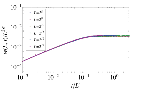
Figure 11: Finite-size scaling collapse of the roughness function $w(L,t)$ defined in Eq. (275). The values of the roughness exponent $\alpha\equiv\chi=1/2$ and the dynamical exponent $z=3/2$ are in the 1D KPZ universality class. Each curve corresponding to a specific system size $L$ is an average over $1000$ noise realizations. The simulations were performed after rescaling the Langevin equation (80) to bring it to dimensionless form. For details of the rescaling and the values of the parameters used in the simulations, see Ref. He et al. (2015). (Copyright (2014) by The American Physical Society.)

The numerical analysis reported in Ref. He et al. (2015) was performed in the regime of weak noise, which is characterized by the absence of phase slips in the spatiotemporal range covered by the simulations. Indeed, the mapping of the condensate dynamics to the KPZ equation (231), in which the phase is regarded as a non-compact variable, does not take into account the possible occurrence of such defects. However, their presence at higher noise levels is expected to affect the scaling properties of driven-dissipative condensates.

V Universal heating dynamics in 1D

The notion of universality is not restricted to systems in thermal equilibrium. As discussed in the previous sections, non-thermal steady states of driven-dissipative systems can show a large variety of universal features, such as scale invariance and effective long-wavelength thermalization. However, in a plethora of setups, aspects of universality can even be found in the time evolution, which approaches a steady state only in the limit $\tau\rightarrow\infty$ Gagel et al. (2014, 2015); Chiocchetta et al. (2015b); Strack (2015); Lesanovsky et al. (2015); Cai and Barthel (2013); Poletti et al. (2013); Schachenmayer et al. (2014). An example which identifies generic, universal features in the far from equilibrium dynamics in a strongly interacting one-dimensional system is discussed in the present section.

The setting we consider here differs from the one in the previous section not only in its focus on time evolution, but also in terms of underlying symmetries. Above we have studied systems that are open in the sense that both energy and particle number were not conserved, witnessed by the absence of the thermal symmetry (cf. Sec. II.4.1) and the quantum phase rotation symmetry (cf. Sec. II.4.4), and leading to a breaking of detailed balance and a low momentum diffusive Goldstone mode (cf. Sec. II.4.6), respectively. Here we consider an open system, where only energy is not conserved, but particle number is. In fact, the absence of energy conservation here is reflected by a permanent inflow of energy into the system. The Lindblad operators are Hermitian in the present case, and this leads to continuous heating and ultimately to an entirely classical, infinite temperature stationary state, described by a density matrix $\rho\sim\mathbf{1}$, where the latter unit matrix is understood in the entire Fock space of the problem. This motivates us to study the time evolution of heating, with a focus on the short time dynamics following initialization in a pure zero temperature ground state, where quantum effects are still present. The presence of particle number conservation leads us to take a different strategy than in the previous sections. Here, accomodating number conservation, which is at the heart of the strongly collective behavior of one dimensional systems, we first map the quantum master equation in the operatorial formalism to an effective long-wavelength description in terms of an open Luttinger liquid. In this way, we can carefully account for the linear sound mode that is expected on the grounds of exact particle number conservation, cf. Sec. II.4.6. Only after this procedure, we perform the mapping to the Keldysh functional integral, similar to our strategy for the spins in Sec. III.

V.1 Heating an interacting Luttinger liquid

Consider a one-dimensional lattice of interacting bosons for which the dynamics is described by the following master equation:

$$\partial_{t}\rho=-i\left[H,\rho\right]+\gamma_{e}\sum_{i}\left[2n_{i}\rho n_{i}-\left\{n^{2}_{i},\rho\right\}\right].$$ (276)

Here, $H$ is a bosonic lattice Hamiltonian, whose long-wavelength physics is described by an interacting Luttinger liquid. For concreteness, one can consider a Bose-Hubbard model in one dimension away from integer filling, with Hamiltonian

$$H=-J\sum_{i}\left(b^{\dagger}_{i}b_{i+1}+b^{\dagger}_{i+1}b_{i}\right)+\tfrac{U}{2}\sum_{i}n_{i}(n_{i}-1),$$ (277)

which describes nearest neighbor hopping of particles with hopping amplitude $J$ and local interactions with interaction energies $U$. The dissipative contributions which drive the system out of equilibrium, are the Hermitian jump operators $n_{i}=b^{\dagger}_{i}b_{i}$, measuring the local particle number in terms of bosonic creation and annihilation operators $b^{\dagger}_{i},b_{i}$. For cold bosonic atoms in optical lattices, these jump operators represent the leading order contribution of dissipation induced by spontaneous emission from the lattice drive laser Pichler et al. (2010) (see also the discussion in Sec. I.3.3), but this kind of dissipation can as well be realized by coupling the bosonic particles to a phonon reservoir with a large effective temperature, which is equivalent to a locally fluctuating chemical potential

$$\begin{split}\mu(x,t)&=\mu_{0}+\delta\mu(x,t),\\ \langle\delta\mu(x,t)\delta\mu(x^{\prime},t^{\prime})\rangle&=\gamma_{e}\delta(t-t^{\prime})\delta(x-x^{\prime}).\end{split}$$

It causes dephasing and leads to a linear increase of the energy in the system, $\langle H\rangle_{t}\propto J\gamma_{e}t$ Pichler et al. (2010, 2013). As a consequence of the linear energy increase, the system will never thermalize and is constantly driven away from equilibrium, approaching the $T\rightarrow\infty$ state described by $\rho\propto\mathbf{1}$ at infinite time $t$. We note that, for hermitean Lindblad operators, $\rho\propto\mathbf{1}$ is always a solution to the quantum master equation.

In order to analyze the heating dynamics for short and transient times, the master equation is transformed to the Luttinger representation on the operatorial level, and only later on we perform the mapping to the Keldysh functional integral. The Luttinger description is valid as long as the occupation of quasi-particle modes does not exceed a critical value, which is determined by the Luttinger cutoff $\Lambda$ Buchhold and Diehl (2015a). Starting with a zero or low temperature initial state to which this applies, there exists a cutoff time $t_{\Lambda}$, up to which the system can be described in terms of Luttinger liquid variables. In this regime, one can take the continuum limit $b_{i}\rightarrow b_{x}$ and express the bosonic operators in a phase and amplitude representation:

$$\begin{split}b_{x}&=\sqrt{\rho_{x}}e^{i\theta_{x}},\\ \rho_{x}&=\rho_{0}+\partial_{x}\phi_{x}/\pi,\end{split}$$ (278)

in terms of the Luttinger variables $\partial_{x}\phi_{x}$ and $\theta_{x}$, which represent smooth density and phase fluctuations and fulfill the commutation relation $\left[\partial_{x}\phi_{x},\theta_{x^{\prime}}\right]=i\pi\delta(x-x^{\prime})$. The long-wavelength description of the Bose-Hubbard model is expressed by the Hamiltonian

$$H=\frac{1}{2\pi}\int_{x}\left[uK\left(\partial_{x}\theta_{x}\right)^{2}-\tfrac{u}{K}\left(\partial_{x}\phi_{x}\right)^{2}+\kappa\left(\partial_{x}\phi_{x}\right)\left(\partial_{x}\theta_{x}\right)^{2}\right],$$ (279)

which describes interacting Luttinger phonons on length scales $x\geq\left(\rho_{0}Um\right)^{-1/2}$, above which a continuum representation of the Hamiltonian is appropriate. For weak interactions, the effective parameters can be estimated to be $u=\left(\tfrac{\rho_{0}U}{m}\right)^{1/2}$, $K=\tfrac{\pi}{2}\left(\tfrac{\rho_{0}}{Um}\right)^{1/2}$. The non-linearity in the Hamiltonian accounts for the leading order quasi-particle scattering term in the low energy regime ($\kappa=1/m$), which is irrelevant in the sense of the renormalization group and does not modify static, equilibrium correlations. However, it is vital for the quantitative description of dynamic correlation functions, and is non-negligible in a non-equilibrium setting where the dynamics is affected by the non-linearity even on a qualitative level. The dissipative part of the master equation becomes quadratic in the Luttinger representation, such that the equation of motion reads

$$\partial_{t}\rho=-i\left[H,\rho\right]+\tfrac{\gamma}{\pi^{2}}\int_{x}\left[2(\partial_{x}\phi_{x})\rho(\partial_{x}\phi_{x})-\left\{(\partial_{x}\phi_{x})^{2},\rho\right\}\right].$$ (280)

This decoherence term is the leading order contribution of a $U(1)$-symmetric (i.e., particle number conserving) decoherence mechanism in one-dimensional quantum wires, which features a linear increase of the energy in time. Furthermore, the $U(1)$ symmetry guarantees the existence of a linear sound mode and permits the transformation to the Luttinger framework in the coherence dominated regime. From a microscopic perspective, it is evident that the Luttinger description has to break down for sufficiently strong decoherence, i.e., after the system has been heated up sufficiently. This breakdown can be estimated by the usual Luttinger criterion $n_{q}<\Lambda/|q|$, and leads to a good estimate for the relevant time scales up to which the dynamics of the system is dominated by coherent sound modes and therefore properly expressed in the Luttinger framework Buchhold and Diehl (2015a). The corresponding time regime is set by the condition $t<u^{2}(\kappa\gamma)^{-1}$.

The quadratic part of the equation of motion is diagonalized by the canonical Bogoliubov transformation

$$\begin{split}\theta_{x}&=\theta_{0}+i\int_{q}(\tfrac{\pi}{2|q|K})^{1/2}(a^{\dagger}_{q}-a^{\phantom{\dagger}}_{-q})e^{-iqx},\\ \phi_{x}&=\phi_{0}-i\int_{q}(\tfrac{\pi K}{2|q|})^{1/2}\mbox{sgn}(q)(a^{\dagger}_{q}+a^{\phantom{\dagger}}_{-q})e^{-iqx},\end{split}$$ (281)

which leads to the master equation

$$\partial_{t}\rho=-i\int_{q}\left[u|q|a^{\dagger}_{q}a^{\phantom{\dagger}}_{q},\rho\right]\\ +\int_{q}\tfrac{\gamma|q|}{\pi K}\left[A^{\phantom{\dagger}}_{q}\rho A^{\dagger}_{q}-\tfrac{1}{2}\{A^{\dagger}_{q}A^{\phantom{\dagger}}_{q},\rho\}\right]-\int_{q}[H^{(3)}_{\mbox{\tiny ph}},\rho].$$ (282)

In this equation, the dissipative part is expressed via the operators $A^{\dagger}_{q}=a^{\dagger}_{q}+a^{\phantom{\dagger}}_{-q}=A^{\phantom{\dagger}}_{-q}$ in terms of bosonic phonon operators $[a^{\phantom{\dagger}}_{q},a^{\dagger}_{p}]=\delta(q-p)$. The cubic Hamiltonian incorporates resonant phonon scattering processes

$$H^{(3)}_{\mbox{\tiny ph}}=3\kappa\sqrt{\tfrac{\pi}{2K}}\int_{q,p}^{\prime}\sqrt{|qp(p+q)}(a^{\dagger}_{p+q}a^{\phantom{\dagger}}_{q}a^{\phantom{\dagger}}_{p}+\mbox{h.c.}),$$ (283)

which conserve momentum and the phonon energy. This is expressed by $\int^{\prime}_{qp}$, which signals to integrate only over configurations $\{p,q\}$ with $|q|+|p|=|p+q|$. The non-resonant processes create only short-lived quantum states which do not contribute in the long time dynamics due to dephasing, and which are therefore not relevant for the forward dynamics of the system.

In the Luttinger representation, the dissipative contribution is quadratic and its effect is a constant population of the individual phonon modes. This can be seen most easily by computing the time evolution of the phonon densities in the quadratic framework, which yields

$$\partial_{t}\langle a^{\dagger}_{q}a^{\phantom{\dagger}}_{q}\rangle_{t} =\tfrac{\gamma|q|}{2\pi K},$$ (284)

$$\partial_{t}\langle a^{\dagger}_{q}a^{\dagger}_{-q}\rangle_{t} =-\tfrac{\gamma|q|}{2\pi K}-2iu|q|\langle a^{\dagger}_{q}a^{\dagger}_{-q}\rangle_{t}.$$ (285)

For a system prepared initially in the ground or finite temperature state, the initial phonon densities are $\langle a^{\dagger}_{q}a^{\phantom{\dagger}}_{q}\rangle_{0}=n_{\mbox{\tiny B}}(u|q|)$ and $\partial_{t}\langle a^{\dagger}_{q}a^{\dagger}_{-q}\rangle_{0}=0$, where $n_{\mbox{\tiny B}}(u|q|)=(e^{\beta u|q|}-1)^{-1}$ is the Bose-Einstein distribution evaluated on-shell. In this case, the solution of Eqs. (284), (285) is

$$\langle a^{\dagger}_{q}a^{\phantom{\dagger}}_{q}\rangle_{t} =n_{\mbox{\tiny B}}(u|q|)+\tfrac{\gamma|q|t}{2\pi K},$$ (286)

$$\langle a^{\dagger}_{q}a^{\dagger}_{-q}\rangle_{t} =\tfrac{\gamma e^{-iu|q|t}}{2\pi uK}\sin(u|q|t).$$ (287)

The first term describes an increase of the phonon density linear in time and momentum and leads to a linear increase of the system energy, i.e., heats up the system according to

$$\Delta E_{t}=\langle H^{(2)}\rangle_{t}-\langle H^{(2)}\rangle_{0}=\tfrac{u\gamma\Lambda^{2}t}{4\pi K}.$$ (288)

Equation (288) relates the effective long-wavelength Luttinger parameters $u,K,\gamma$ of the heating setup to the macroscopic heating rate $\partial_{t}\Delta E_{t}$ via the microscopic cutoff $\Lambda$. Since this heating rate is not model specific but depends on the individual realization of the heating dynamics, it is not surprising that it depends on macroscopic and microscopic parameters. In this sense, Eq. (288) should be viewed as the definition of the effective heating parameter $\gamma$ for a generic model in the presence of heating Buchhold and Diehl (2015a).

The off-diagonal phonon density oscillates in the complex plane, thereby taking absolute values $|\langle a^{\dagger}_{q}a^{\dagger}_{-q}\rangle_{t}|\leq\tfrac{\gamma}{2\pi uK}$, which are negligibly small in the weak heating regime $\gamma\ll uK$, i.e., in the coherence dominated dynamics. It is therefore sufficient to consider only the diagonal elements in the phonon basis when extending the analysis to the interacting model.

The jump operators in the microscopic master equation (276) are the Hermitian, local density operators $n_{i}$, which preserve the $U(1)$ invariance of the dynamics even in the presence of dissipation. This leads to a decay of the off-diagonal elements of the density matrix, i.e., to decoherence in the local number state representation, and an evolution of the density matrix towards its diagonal ensemble. In the Luttinger representation, this decoherence expresses itself in a permanent production of photons (286), i.e. a permanent heating of the Luttinger liquid, which features no compensation mechanism in the quadratic sector and the consequent lack of a well defined steady state. The energy increases constantly, which will lead to an obvious breakdown of the Luttinger description as soon as the energy stored in the long-wavelength modes exceeds a critical value. At this point, the dynamics is no longer dominated by the coherences of $\rho$ but by its diagonal elements, including the breakdown of superfluidity and quasi-long range order.

The way in which energy is distributed amongst the long-wavelength modes by the heating (284) is not typical for an interacting system at low energies, since it deviates strongly from a Bose-Einstein distribution and the associated detailed balance of energy. The phonon scattering terms in $H^{(3)}_{\mbox{\tiny ph}}$ favor detailed balance and strongly modify the actual distribution function compared to (286), which makes them non-negligible in the present non-equilibrium setting.

V.2 Kinetic equation

In order to determine the time evolution of the excitation densities in interacting systems out of equilibrium, a common and often successful strategy is the so-called kinetic equation approach Kamenev (2011) (for an application to periodically driven Floquet systems, cf. Ref. Genske and Rosch (2015)), which determines the time evolution of the distribution function of the excitations in terms of the system’s self-energies. For the present setup, this approach has to be modified in order to take into account the driven-dissipative nature of the system and the resonant character of the interactions. The latter lead to a breakdown of perturbation theory and require non-perturbative techniques beyond one-loop corrections. A detailed derivation and discussion of the applicability and limitations of such an approach can be found in Buchhold and Diehl (2015b, a). Other forms of kinetic equations for interacting Luttinger liquids, which focus on a different set of non-equilibrium conditions, include a perturbative treatment of phonon backscattering terms, resulting from additional disordered or lattice potentials Tavora et al. (2014); Tavora and Mitra (2013), as well as a treatment of cubic phonon interactions in the presence of a smooth background potential and a curved phonon dispersion Protopopov et al. (2014).

The quantity of interest in this section is the time-dependent occupation of phonon modes $n_{q,t}=\langle a^{\dagger}_{q}a_{q}\rangle_{t}$ in the presence of heating and phonon scattering. For bosonic modes and in the steady state, the occupation of the modes is related to the Keldysh Green’s function via

$$i\int_{\omega}G^{K}_{q,\omega}=2n_{q}+1.$$ (289)

For a system in thermal equilibrium, $n_{q}=n_{\text{B}}(\epsilon_{q},T)$ is the Bose distribution function, see Sec. II.4.1, while for a general non-equilibrium steady state, $n_{q}$ is a positive function, which has to be determined from the specific context. One can now introduce the hermitian distribution function $F_{q,\omega}$ as in Eq. (72), but generalized to a system with a continuum of momentum modes. In terms of the hermitian distribution function, the anti-hermitian Keldysh Green’s function can be parameterized according to

$$G^{K}_{q,t,t^{\prime}}=\left(G^{R}_{q}\ \tilde{\circ}\ F_{q}-F_{q}\ \tilde{\circ}\ G^{A}_{q}\right)_{t,t^{\prime}}.$$ (290)

Here, $G^{R}_{q},\ G^{A}_{q}=\left(G^{R}_{q}\right)^{\dagger}$ and $F_{q}$ are two-time functions evaluated at equal momentum $q$ and $\tilde{\circ}$ represents the convolution with respect to time and matrix multiplication according to the Nambu structure of the Green’s functions. For a system, which is diagonal in Nambu space, $\tilde{\circ}=\circ$ reduces to a simple multiplication. In the presence of off-diagonal occupations, i.e. for $\langle a^{\dagger}_{-q}a^{\dagger}_{q}\rangle\neq 0$, the operation $\tilde{\circ}$ has to respect the symplectic structure of bosonic Nambu space and is promoted to $\tilde{\circ}=\sigma^{z}\circ$, as described in Ref. Buchhold and Diehl (2015b). For a bosonic system in steady state, all terms in (290) are time-translational invariant and Fourier transformation yields

$$G^{K}_{q,\omega}=G^{R}_{q,\omega}\sigma^{z}F_{q,\omega}-F_{q,\omega}\sigma^{z}G^{A}_{q,\omega}.$$ (291)

In contrast, for a system out of equilibrium undergoing a non-trivial time evolution, the mode occupations $n_{q,t}$ remain well defined, but Eq. (290) is not time-translational invariant anymore. One then has to find a representation for the Green’s functions and $F$, which reveals the time-dependent occupations. This is done in the following, leading to the Wigner representation of the bosonic distribution function.

A convenient parameterization of non-equilibrium correlation and response functions is the so-called Wigner representation in time, which introduces a forward and a relative time coordinate ($t,\delta$) for the phonon Green’s functions, according to

$$G^{R}_{q,t,\delta} =-i\theta(\delta)\langle[a^{\phantom{\dagger}}_{q,t+\delta/2},a^{\dagger}_{q,t-\delta/2}]\rangle,$$ (292)

$$G^{K}_{q,t,\delta} =-i\langle\{a^{\phantom{\dagger}}_{q,t+\delta/2},a^{\dagger}_{q,t-\delta/2}\}\rangle.$$ (293)

A two-time function $C(t_{1},t_{2})$ can always be transformed to Wigner coordinates, $C(t_{1},t_{2})=C(t,\delta)$, by defining $t=\tfrac{t_{1}+t_{2}}{2}$ and $\delta=t_{1}-t_{2}$. Here, the explicit dependence on $t$ expresses the forward time evolution of non-equilibrium systems, while for equilibrium systems in the presence of time-translational invariance, the forward time dependence of generic two-time functions just drops out, $C(t,\delta)\equiv C(0,\delta)$, for all $t$. In Wigner coordinates, the parametrization of the Keldysh correlation function is

$$G^{K}_{q,t,\delta}=\left(G^{R}_{q}\circ F_{q}-F_{q}\circ G^{A}_{q}\right)_{t,\delta}.$$ (294)

Here, we choose to neglect the subleading off-diagonal contributions according to the above discussion, and consider only diagonal modes in Nambu space. Eq. (294) contains the full Green’s functions of the system, which can be expressed via the Dyson relation in terms of the self-energies $\Sigma^{R/A/K}$,

$$\left(\begin{array}[]{cc}G^{K}&G^{R}\\ G^{A}&0\end{array}\right)^{-1}=\left(\begin{array}[]{cc}0&G_{0}^{A}-\Sigma^{A}\\ G_{0}^{R}-\Sigma^{R}&-\Sigma^{K}\end{array}\right).$$ (299)

The self-energies $\Sigma^{R/A/K}$ represent the correction to the bare Green’s functions $G^{R/A}_{0}=(i\partial_{t}-u|q|)^{-1}$ due to phonon scattering and heating events. Inserting the Dyson representation into Eq. (294), it can be inverted and rearranged to read

$$\partial_{t}F_{q,t,\delta}=i\Sigma^{K}_{q,t,\delta}-i\left(\Sigma^{R}_{q}\circ F_{q}-F_{q}\circ G^{A}_{q}\right)_{t,\delta}.$$ (300)

Here, the notion $(...)_{t,\delta}$ expresses the fact that the whole expression in brackets should be transformed to Wigner coordinates after performing the convolution $\Sigma^{R}_{q}\circ F_{q}\equiv\int_{t^{\prime}}\Sigma^{R}_{q,t_{1},t^{\prime}}F_{q,t^{\prime},t_{2}}$ in ordinary time representation. The functionals $\Sigma^{R/A/K}$ are the self-energies in the retarded, advanced, and Keldysh sectors, which incorporate the effect of interactions and the heating on the quadratic sector. The temporal derivative on the LHS of (300) is the Wigner representation of the bare, non-interacting Green’s functions without heating. Taking the Fourier transform of Eq. (300) with respect to the relative time coordinate $\delta$ yields the Wigner representation of the distribution function

$$F_{q,t,\omega}=\int_{\delta}e^{i\omega\delta}F_{q,t,\delta},$$ (301)

for which

$$\partial_{t}F_{q,t,\omega}=i\Sigma^{K}_{q,t,\omega}-i\left(\Sigma^{R}\circ F-F\circ\Sigma^{A}\right)_{q,t,\omega}.$$ (302)

The corresponding transformation for the convolution inside the parenthesis is

$$\left(\Sigma^{R}\circ F\right)_{q,t,\omega}=\Sigma^{R}_{q,t,\omega}e^{\frac{i}{2}\left(\overset{\leftarrow}{\partial}_{t}\overset{\rightarrow}{\partial}_{\omega}-\overset{\leftarrow}{\partial}_{\omega}\overset{\rightarrow}{\partial}_{t}\right)}F_{q,t,\omega}.$$ (303)

Its explicit evaluation is nontrivial and in most cases simply impossible. However, it is possible to approximate the complex exponential by the leading order expansion for many typical relaxation dynamics Kamenev (2011). In order to understand Eq. (303), one should take a closer look at its expansion up to first order in derivatives:

$$\left(\Sigma^{R}\circ F\right)_{q,t,\omega}=\Sigma^{R}_{q,t,\omega}F_{q,t,\omega}\left(1-\tfrac{i}{2}\tfrac{\partial_{t}F_{q,t,\omega}}{F_{q,t,\omega}}\tfrac{\partial_{\omega}\Sigma^{R}_{q,t,\omega}}{\Sigma^{R}_{q,t,\omega}}+(\omega\leftrightarrow t)\right)+O(\partial^{2}).$$ (304)

The ratio $\kappa^{f}_{q}\equiv\left|\tfrac{\partial_{t}F_{q,t,\omega}}{F_{q,t,\omega}}\right|$ is the rate with which the distribution $F$ is changing in forward time, i.e., the forward time evolution rate, which is determined by the interplay between heating and collective quasi-particle scattering. On the other hand, $\left(\kappa^{r}_{q}\right)^{-1}\equiv\left|\tfrac{\partial_{\omega}\Sigma^{R}_{q,t,\omega}}{\Sigma^{R}_{q,t,\omega}}\right|$ is identified with the inverse rate of the relative time dynamics, which is dominated by fast single phonon propagation. As a consequence $\kappa^{r}_{q}\gg\kappa^{f}_{q}$ and the correction terms in (304) can be safely neglected. This is a typical situation for many kinetic equation approaches and is termed the Wigner approximation. For the present setup, a more careful analysis has shown that the Wigner approximation is indeed satisfied as long as the Luttinger representation of the problem is valid Buchhold and Diehl (2015a).

In order to project Eq. (302) onto the quasi-particle densities, it is multiplied by the spectral function $\mathcal{A}_{q,t,\omega}=iG^{R}_{q,t,\omega}-iG^{A}_{q,t,\omega}$, followed by a subsequent integration over frequencies $\omega$. The spectral function fulfills the sum rules

$$\int_{\omega}\mathcal{A}_{q,t,\omega} = \langle[a^{\phantom{\dagger}}_{q,t,0},a^{\dagger}_{q,t,0}]\rangle=1,$$ (305)

$$\int_{\omega}\mathcal{A}_{q,t,\omega}F_{q,t,\omega} \overset{\text{Wigner approx.}}{=} \int_{\omega}\left(\mathcal{A}\circ F\right)_{q,t,\omega}=G^{K}_{q,t,0}=2n_{q,t}+1,\ \ \ \ \ \ \ \ \$$ (306)

with $n_{q,t}=\langle a^{\dagger}_{q,t}a^{\phantom{\dagger}}_{q,t}\rangle$ being the phonon density. Applying this to Eq. (302) in the Wigner approximation yields

$$\partial_{t}n_{q,t}=\tfrac{i}{2}\int_{\omega}\left(\Sigma^{K}_{q,t,\omega}-\Sigma^{R}_{q,t,\omega}F_{q,t,\omega}+\Sigma^{A}_{q,t,\omega}F_{q,t,\omega}\right)\mathcal{A}_{q,t,\omega}.$$ (307)

For well defined quasi-particles, i.e., excitations with a well defined energy-momentum relation, the spectral function reflects the well-defined structure of the excitations and is sharply peaked at the quasi-particle dispersion $\omega=u|q|$, with a typical width $\sigma^{R}_{q,t}\ll u|q|$, which is the imaginary part of the self-energy evaluated on the mass shell $\sigma^{R}_{q,t}=-\mbox{Im}(\Sigma^{R}_{q,t,u|q|})$. If this is the case, the full self-energies in Eq. (307) multiplied with the spectral function can be approximated by their on-shell values, as they are expected to vary only smoothly in the region where $\mathcal{A}$ is non-zero. The approximation $\Sigma^{R/A/K}_{q,t,\omega}\mathcal{A}_{q,t,\omega}\approx\Sigma^{R/A/K}_{q,t,u|q|}\mathcal{A}_{q,t,\omega}$ is called the quasi-particle approximation and in the present case, similar to the Wigner approximation, it is applicable in the entire Luttinger regime Buchhold and Diehl (2015a, b). The latter is a consequence of the subleading, RG-irrelevant nature of the interactions, which lead to self-energies $\sigma^{R}_{q,t}\ll u|q|$. Performing the quasi-particle approximation, Eq. (307) obtains the simple form

$$\partial_{t}n_{q,t}=\tilde{\sigma}^{K}_{q,t}-\sigma^{R}_{q,t}(2n_{q,t}+1).$$ (308)

In this equation, the anti-Hermitian Keldysh self-energy $\Sigma^{K}_{q,t,\omega}$ has been replaced by its on-shell value $\Sigma^{K}_{q,t,u|q|}=-2i\tilde{\sigma}^{K}_{q,t}$, with the real function $\tilde{\sigma}^{K}_{q,t}$.

The kinetic equation (308) describes the time evolution of the phonon density $n_{q,t}$ in terms of the on-shell self-energies $\sigma^{R},\tilde{\sigma}^{K}$, which in turn are determined by both the interactions and the heating term. In order to identify the contribution from the heating, one has to identify the impact of the dissipative contribution in Eq. (282) on the action $S$. Following the steps in Sec. II.1 carefully and setting the off-diagonal density contributions to zero, according to Eq. (286), the dissipative contribution to the microscopic action $S$ is

$$S_{D}=i\int_{p,t}\tfrac{\gamma|p|}{\pi K}a^{*}_{q,p,t}a_{q,p,t}.$$ (309)

Here, $p$ is the momentum variable and $q$ labels the quantum component of the Keldysh field variable. The dissipation thus enters the action only in the quantum-quantum sector and does not modify the spectrum in the quantum-classical sector. This is again a consequence of the Hermitian nature of the Lindblad operators, which lead to a continuously increasing occupation of phonons but do not introduce a compensating dissipative mechanism in the retarded and advanced sector of the action . This is drastically different from the situation in the models of Secs. III (cf. Eqs. (141) and (140)) and IV (cf. Eqs. (236) and (237)), where the interplay of dissipation in the retarded/advanced sectors and fluctuation or noise in the Keldysh sector of the action lead to non-equilibrium fluctuation-dissipation relations describing well-defined stationary states different from the trivial state $\rho\propto\mathbf{1}$.

With the form of (309), the Keldysh self-energy is $\tilde{\sigma}^{K}_{q,t}=\tfrac{\gamma|p|}{2\pi K}+\sigma^{K}_{q,t}$, where the bare $\sigma^{K}_{q,t}$ in this form is determined by the interactions alone. The resulting kinetic equation consists of three contributions

$$\partial_{t}n_{q,t}=\underbrace{\tfrac{\gamma|q|}{2\pi K}}_{\text{in-term heating}}+\underbrace{\sigma^{K}_{q,t}}_{\text{in-term scattering}}-\underbrace{\sigma^{R}_{q,t}(2n_{q,t}+1)}_{\text{out-term scattering}}.$$ (310)

The first term represents the population of phonon modes due to the constant heating term, while the second and the third term are effects of the elastic collisions redistributing energy. The second term, proportional to the Keldysh self-energy, describes scattering of phonons into the mode $q$ due to the interactions, while the third term, proportional to the retarded self-energy, describes scattering of phonons out of the mode $q$, and is therefore directly proportional to $n_{q,t}$. Setting the interactions to zero, both self-energies $\sigma^{R/K}=0$ vanish and only the heating term remains, rendering the time evolution of the phonon density in the absence of interactions into Eq. (284).

The kinetic equation (310) represents the foundation of the analysis of the non-equilibrium dynamics in the presence of heating and phonon scattering. In order to solve for the time-evolution of the phonon densities, one has to compute the self-energies $\sigma^{R/K}_{q,t}$ for each momentum mode and at each time step. The self-energies have to be determined by a non-perturbative approach, which we discuss in the following.

V.3 Self-consistent Born approximation

For an interacting model of resonantly scattering phonons, the phonon self-energies are functionals of the phonon density, such that the RHS of (310) contains an implicit, non-linear dependence on $n_{q,t}$. In order to make this implicit dependence explicit, the self-energies are typically evaluated perturbatively at one loop order and higher order corrections to the time evolution are neglected Kamenev (2011). However, for the present scenario, the interactions are resonant, i.e., describe scattering events inside a continuum of degenerate states, and therefore perturbative computations diverge at any order. This defines the need for non-perturbative approaches to compute the phonon self-energies, the simplest of which is the so-called self-consistent Born approximation, which we discuss in the following.

The Keldysh action for interacting Luttinger liquids with heating is composed of a dissipative part $S_{D}$, which has been discussed in Eq. (309), and a Hamiltonian part $S_{H}$, which results from the Hamiltonian dynamics in Eqs. (282), (283). In the Keldysh representation, the action is

$$S=\int_{p,t}(a^{*}_{c,p,t},a^{*}_{q,p,t})\left(\begin{array}[]{cc}0&i\partial_{t}-u|p|-i0^{+}\\ i\partial_{t}-u|p|+i0^{+}&i\tfrac{\gamma|p|}{\pi K}\end{array}\right)\left(\begin{array}[]{c}a_{c,p,t}\\ a_{q,p,t}\end{array}\right)\\ +\int^{\prime}_{p,k,t}v(p,k)\Big{[}2a^{*}_{c,k+p,t}a_{c,k,t}a_{q,p,t}\\ +a^{*}_{q,k+p,t}\Big{(}a_{c,k,t}a_{c,p,t}+a_{q,k,t}a_{q,p,t}\Big{)}+\text{h.c.}\Big{]}$$ (311)

with the vertex function $v(p,k)=3\kappa\sqrt{\tfrac{\pi}{2K}|pk(p+k)}$. One way of computing the one-loop self-energy is to determine the one-loop correction to the effective action $\Gamma[a^{*}_{\alpha},a_{\alpha}]$ defined in Eq. (39) for general bosonic fields $\Phi$. The effective action in the absence of an external source is defined as

$$e^{i\Gamma[a^{*}_{\alpha},a_{\alpha}]}=\int\mathscr{D}[\delta a^{*}_{\alpha},\delta a_{\alpha}]\,e^{iS[a^{*}_{\alpha}+\delta a^{*}_{\alpha},a_{\alpha}+\delta a_{\alpha}]},$$ (312)

and fulfills the equation of motion $\frac{\delta\Gamma[a^{*}_{\alpha},a_{\alpha}]}{\delta a^{*}_{\alpha}}=\frac{\delta\Gamma[a^{*}_{\alpha},a_{\alpha}]}{\delta a_{\alpha}}=0$. The one-loop effective action is then obtained by expanding the action $S$ up to second order in the fluctuation fields and subsequently integration over the fluctuations

$$e^{i\Gamma^{(\text{1-loop})}[a^{*}_{\alpha},a_{\alpha}]} = e^{iS[a^{*}_{\alpha},a_{\alpha}]}\int\mathscr{D}[\delta a^{*}_{\alpha},\delta a_{\alpha}]\,e^{\frac{i}{2}(\delta a^{*}_{\alpha},\delta a_{\alpha})S^{(2)}[a^{*}_{\alpha},a_{\alpha}](\delta a_{\alpha},\delta a^{*}_{\alpha})^{T}}$$ (313)

$$= e^{iS[a^{*}_{\alpha},a_{\alpha}]+\frac{1}{2}\text{Tr}\log\left(S^{(2)}[a^{*}_{\alpha},a_{\alpha}]\right)}.$$

This identifies the one-loop effective action

$$\Gamma^{(\text{1-loop})}[a^{*}_{\alpha},a_{\alpha}]=S[a^{*}_{\alpha},a_{\alpha}]-\tfrac{i}{2}\text{Tr}\log\left(S^{(2)}[a^{*}_{\alpha},a_{\alpha}]\right)$$ (314)

in terms of the microscopic action $S$ and its second variation with respect to the fields

$$S^{(2)}[a^{*}_{\alpha},a_{\alpha}]=\left(\begin{array}[]{cc}\frac{\delta^{2}S}{\delta a^{*}_{\alpha}\delta a_{\alpha^{\prime}}}&\frac{\delta^{2}S}{\delta a^{*}_{\alpha}\delta a^{*}_{\alpha^{\prime}}}\\ \frac{\delta^{2}S}{\delta a_{\alpha}\delta a_{\alpha^{\prime}}}&\frac{\delta^{2}S}{\delta a_{\alpha}\delta a^{*}_{\alpha}}\end{array}\right).$$ (317)

In order to determine the correction to the bare action, the logarithm in Eq. (314) is expanded in powers of the fields $a^{*}_{\alpha},a_{\alpha}$. The quadratic self-energy is the second order expansion of the logarithm and its matrix elements are determined by the integrals

$$\Sigma^{R}_{Q} =2i\int_{P}^{\prime}G^{K}_{P}\left(v^{2}(q,-p)G^{R}_{Q-P}+v^{2}(p,-q)G^{A}_{P-Q}+v^{2}(p,q)G^{R}_{P+Q}\right),$$ (318)

$$\Sigma^{K}_{Q} =2i\int_{P}^{\prime}\left[v^{2}(q-p)\left(G^{K}_{P}G^{K}_{Q-P}+G^{R}_{P}G^{R}_{Q-P}+G^{A}_{P}G^{A}_{Q-P}\right)\right.$$

$$\left.+2v^{2}(p,q)\left(G^{K}_{P+Q}G^{K}_{P}+G^{A}_{P+Q}G^{R}_{P}+G^{R}_{P+Q}G^{R}_{P}\right)\right],$$ (319)

where we used the collective indices $Q=(q,\omega),P=(p,\nu)$ for momentum and relative frequency. In Wigner approximation, the Green’s functions are diagonal in forward time and therefore evaluated at equal forward time $t$. The integrals in (318), (319) are performed only over resonant momentum configurations, see the discussion around Eq. (283). In perturbation theory, the Green’s functions under the integral are the bare, non-interacting Green’s functions $G^{R}_{Q}=\left(\omega-u|q|+i0^{+}\right)^{-1}$, which diverge on the mass-shell $\omega=u|q|$ and lead to a summation of infinities for the self-energy. On the other hand, in self-consistent Born approximation, the bare Green’s functions in Eqs. (318), (319) are replaced by the full Green’s functions $G^{R}_{Q}=\left(\omega-u|q|-\Sigma^{R}_{Q}\right)^{-1}$. As a consequence, the on-shell Green’s function is regularized by the self-energy $\Sigma^{R}$ and takes the value

$$G^{R}_{q,u|q|}=-\left(\Sigma^{R}_{q,u|q|}\right)^{-1}=-i\left(\sigma^{R}_{q}\right)^{-1}.$$ (320)

Inserting (320) in the definition for the retarded self-energy and evaluating the self-energy on-shell, one obtains

$$\sigma^{R}_{q,t}=v_{0}^{2}\int_{0<p}\left(\tfrac{\partial_{t}n_{p,t}}{\sigma^{R}_{q,t}}+2n_{p,t}+1\right)\left(\frac{qp(q-p)}{\sigma^{R}_{p,t}+\sigma^{R}_{q-p,t}}+\frac{pq(p+q)}{\sigma^{R}_{p,t}+\sigma^{R}_{p+q,t}}\right)$$ (321)

with the vertex prefactor $v_{0}=v(1,1)$, cf. the definition below Eq. 311. A similar equation is obtained for the Keldysh on-shell self-energy $\sigma^{K}_{q,t}$. Inserting Eq. (321) and the result for the Keldysh self-energy, which we do not discuss here but can be found in Ref. Buchhold and Diehl (2015b), into the kinetic equation (310), one finds

$$\partial_{t}n_{q}=\frac{\gamma|q|}{2\pi K}\\ +2v_{0}^{2}\int_{0<p<q}\frac{pq(q-p)(n_{p}n_{q-p}-n_{q}(1+n_{p}+n_{q-p}))}{\sigma^{R}_{q}+\sigma^{R}_{p}+\sigma^{R}_{q-p}}\\ +4v_{0}^{2}\int_{0<p}\frac{pq(q+p)(n_{q+p}(n_{q}+n_{p}+1)-n_{q}n_{p})}{\sigma^{R}_{q}+\sigma^{R}_{p}+\sigma^{R}_{q+p}}.$$ (322)

The kinetic equation (322) and the equation for the on-shell self-energy (321) determine the forward time evolution of the system’s phonon density $n_{q,t}$ and self-energy $\sigma^{R}_{q,t}$ in a self-consistent manner. For a general phonon density, both equations have to be solved iteratively according to the scheme depicted in Fig. 12.

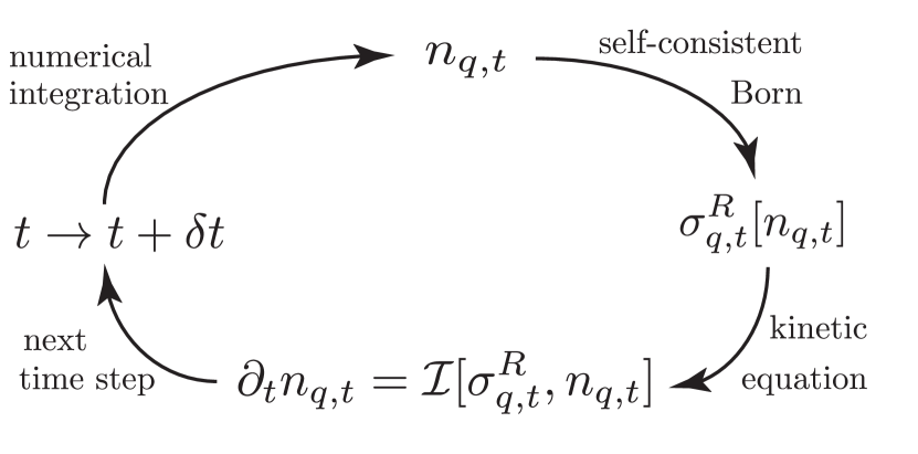
Figure 12: Illustration of the iterative process to compute the time evolution of the phonon density $n_{q,t}$. For a specific forward time $t$, the on-shell self-energy $\sigma^{R}_{q,t}$ is determined via Eq. (321) and subsequently the result is inserted into the kinetic equation (322). In order to integrate the phonon density, a Runge-Kutta solver for differential equations is used, which determines $n_{q,t}$ numerically.

Before the numerical results for dynamics in the presence of heating, i.e., the numerical solution of Eqs. (321), (322), are discussed, it is useful to study certain limiting cases. This facilitates the understanding of the numerical results in the subsequent section.

V.3.1 Kinetics for small momenta

For sufficiently small momenta $q\ll 1$, the kinetic equation simplifies considerably. In this case, the second line of Eq. (322) can be discarded completely, since the integral is performed over a very small momentum interval $0<p<q$. On the other hand, for the integral in the third line of Eq. (322), all terms $(q+p)\approx p$ for the dominant part of the integral. Therefore

$$\partial_{t}n_{q,t}=|q|\left(\frac{\gamma}{2\pi K}+\mathcal{J}_{t}\right),$$ (323)

where the time-dependent integral $\mathcal{J}_{t}$ is $q$-independent and reads

$$\mathcal{J}_{t}=2v_{0}^{2}\int_{0<p}\frac{p^{2}n_{p}(n_{p}+1)}{\sigma^{R}_{p}}.$$ (324)

As a consequence, the resulting change of the phonon density for small momenta $|q|$ is linearly proportional to $|q|$, i.e.

$$n_{q,t}=n_{q,0}+|q|\left(\frac{\gamma t}{2\pi K}+\int_{0<t^{\prime}<t}\mathcal{J}_{t^{\prime}}\right).$$ (325)

The momentum regime $0<|q|<q_{2}$, defined as the regime where the non-linear contributions in $|q|$ are negligible, depends on the actual value of the phonon density $n_{q,t}$, and has to be determined for each specific scenario individually. However, the existence of $q_{2}$ is guaranteed by the above general arguments, and the fact that $\partial_{t}n_{q=0,t}=0$ for all times $t$. The latter is a consequence of the $U(1)$ symmetry of the present setup and the global particle number conservation, as discussed in Buchhold and Diehl (2015b).

V.3.2 Scaling of the self-energy

The fact that the present system is described by a $U(1)$-invariant, massless field theory is reflected by the absence of a scale in the self-energy equation (321). One important consequence is that $\sigma^{R}_{q,t}\overset{q\rightarrow 0}{\rightarrow}0$ generically, i.e., the generation of a mass gap is forbidden by symmetry. A further consequence of Eq. (321) is that, whenever the term in brackets obeys a scaling law,

$$\tfrac{\partial_{t}n_{p}}{\sigma^{R}_{p}}+2n_{p}+1\sim\gamma_{n}|p|^{\eta_{n}},$$ (326)

the solution for the self-energy will be a scaling function $\sigma^{R}_{q}=\gamma_{R}|p|^{\eta_{R}}$ as well. Inserting this scaling ansatz in Eq. (321) yields

$$\gamma_{R}|p|^{\eta_{R}}=\frac{v_{0}^{2}\gamma_{n}}{\gamma_{R}}|p|^{4+\eta_{n}-\eta_{R}}\mathcal{I}_{\eta_{n},\eta_{R}}$$ (327)

and identifies

$$\eta_{R}=2+\frac{\eta_{n}}{2}\text{ and }\gamma_{R}=v_{0}\sqrt{\gamma_{n}\mathcal{I}_{\eta_{n},\eta_{R}}}.$$ (328)

The dimensionless integral $\mathcal{I}_{\eta_{n},\eta_{R}}$ is defined as

$$\mathcal{I}_{\eta_{n},\eta_{R}}=\int_{0<x}x^{\eta_{n}}\left(\frac{x(1-x)}{x^{\eta_{R}}+|1-x|^{\eta_{R}}}+\frac{x(1+x)}{x^{\eta_{R}}+(1+x)^{\eta_{R}}}\right),$$ (329)

and depends only on the exponents $\eta_{R},\eta_{n}$. This self-energy integral is dominated by contributions around $x=1$ and converges for all physically reasonable phonon densities. In this sense, the scaling behavior is universal, i.e. robust against the influence from high energy modes Buchhold and Diehl (2015b, a).

V.4 Heating and universality

With the preparations from the previous sections, one can simulate the heating dynamics of an interacting Luttinger liquid in terms of the time dependent phonon population $n_{q,t}$ and self-energy $\sigma^{R}_{q,t}$, as has been done in Refs. Buchhold and Diehl (2015b, a). Considering the system initially to be in the ground state, the simulation is initialized with a phonon density $n_{q,t=0}=0$, which for $t>0$ is continuously increased due to heating. The central result of the analysis is a scaling solution for the self-energies $\sigma^{R}_{q,t}\sim|q|^{\eta_{R}}$ with a new non-equilibrium exponent $\eta_{R}=5/3$, which is observable in the long-wavelength regime, i.e., on distances $x>x_{\text{th}}(t)$. Here, $x_{\text{th}}(t)$ marks a thermal distance, below which the dynamics is dominated by thermalized short distance modes and above which the phonon density increases linearly in momentum $n_{q,t}\sim|q|$, as it was the case for the bare heating (284). The thermal distance increases sub-ballistically $x_{\text{th}}(t)\sim t^{4/5}$ in time, with a characteristic heating exponent $\eta_{h}=4/5$, while at the same time, the effective temperature describing the distribution of the short distance modes increases linearly in time $T(t)\sim t$.

V.4.1 Phonon densities

The results of a numerical simulation of the phonon densities are shown in Fig. 13. One can clearly identify the crossover from an interaction dominated thermal regime with $n_{q,t}=\frac{T(t)}{u|q|}$ at large momenta to a heating dominated regime with $n_{q,t}\sim|q|$. The crossover momentum between the two regimes represents the inverse thermal length $(x_{\text{th}}(t))^{-1}\sim t^{-4/5}$.

In the large momentum regime, the dominant contribution to the kinetic equation is the collision term, which establishes an approximate detailed balance between phonon absorption and emission in the presence of the heating. This is expressed by the evolution of the phonon density towards a Bose-Einstein distribution, which is the fixed point of the collision term alone. In this regime $n_{q,t}=n_{\text{B}}(u|q|,T(t))\approx\frac{T(t)}{u|q|}$ with very good agreement and the only indicator of the permanent heating is the continuously increasing temperature $T(t)\sim t$.

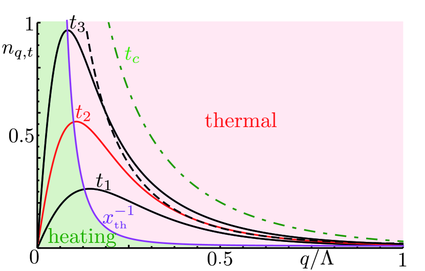
Figure 13: Time evolution of the phonon density $n_{q,t}$ in a sequence $(t_{1},t_{2},t_{3})=(2,3,4)\cdot\frac{10}{v_{0}\Lambda^{2}}$ in terms of $q/\Lambda$ and for a heating rate $\gamma=0.06v_{0}\Lambda$. In the heating regime, for small momenta, the distribution increases linearly in momentum $n_{q,t}\sim|q|$, while it decreases as $n_{q,t}\sim 1/|q|$ in the interaction dominated thermal regime. The crossover $x_{\text{th}}^{-1}\sim t^{-4/5}$ approaches zero as time evolves. The dashed line represents a Bose-Einstein distribution corresponding to the phonon density at $t=t_{3}$. The dash-dotted line indicates $n_{B}(T(t_{c}))$ at the time $t_{c}$, for which the Luttinger description breaks down, i.e., $T(t_{c})=u\Lambda$.

This is contrasted by the evolution of the phonon density in the low momentum regime, which is dominated by strong phonon production. In this regime, the scattering of high-momentum phonons into low-momentum modes enhances the effect of the heating and leads, due to the structure of the vertex, to an increase of the linear production rate according to Eq. (323). The pinning of the phonon occupation of the $q=0$ mode is an exact result for the underlying $U(1)$-symmetric, i.e. particle number conserving dynamics. It can be shown that the phonon number fluctuations in the zero momentum mode are proportional to the fluctuations of the global particle number in the system, see Ref. Buchhold and Diehl (2015a), and consequently they are integrals of motion for a $U(1)$-symmetry preserving dynamics. The pinning effect for the low momentum distribution at $n_{q=0,t}=n_{q=0,0}$ leads to a very slow, sub-ballistic thermalization of the low momentum regime, since the formation of the typical, thermal Rayleigh-Jeans divergence $n_{q,t}\sim 1/|q|$ is only achieved by the scaling of the inverse thermal length $(x_{\text{th}}(t))^{-1}$ to zero, instead of a direct filling of these modes.

V.4.2 Non-equilibrium scaling

Away from the crossover scale $q\neq x_{\text{th}}^{-1}$, deep in the heating or thermal regimes, the phonon density exhibits scaling behavior and can be written as

$$n_{q,t}=\left\{\begin{array}[]{cl}c(t)|q|&\text{ for }|q|\ll x_{th}^{-1}\\ \frac{T(t)}{u|q|}&\text{ for }|q|\gg x_{th}^{-1}\end{array}\right.,$$ (332)

where the functions $c(t)$, $T(t)$ have to be determined numerically. In these regimes, according to Sec. V.3.2, one finds scaling behavior of the phonon self-energy as well. The corresponding scaling exponent is determined by

$$f_{q,t}\equiv\frac{\partial_{t}n_{q,t}}{\sigma^{R}_{q,t}}+2n_{q,t}+1\sim|q|^{\eta_{n}}.$$ (333)

In the heating dominated regime, $n_{q,t}=c(t)|q|$ and therefore

$$f_{q,t}=\frac{c^{\prime}(t)}{\gamma_{R}}|q|^{1-\eta_{R}}+c(t)|q|+1\overset{\eta_{R}>1}{\rightarrow}\frac{c^{\prime}(t)}{\gamma_{R}}|q|^{1-\eta_{R}}$$ (334)

for small momenta, since $\eta_{R}>1$ is guaranteed by the subleading nature of the interactions. This directly implies $\eta_{n}=1-\eta_{R}$ and a super-diffusive exponent $\eta_{R}=\frac{5}{3}$ in this regime, which lacks any equilibrium counterpart.

On the other hand, in the large momentum regime $f_{q,t}$ is obviously dominated by the term proportional to $n_{q,t}$ and $\eta_{n}=-1$, which leads to the known thermal equilibrium exponent $\eta_{R}=\frac{3}{2}$ Andreev (1980) and a thermal scaling behavior for large momenta not only in the distribution function but also in the self-energy. The crossover between the two scaling regimes can be estimated by equating the two relevant terms, which tend to dominate $f_{q,t}$ in the corresponding regimes. This yields

$$\frac{\partial_{t}n_{q_{\text{th}}}}{2n_{q_{\text{th}}}+1}=\sigma^{R}_{q_{\text{th}}},$$ (335)

for $q_{\text{th}}=x_{\text{th}}^{-1}$ and can be used to analytically estimate the scaling of $x_{\text{th}}(t)$ in time Buchhold and Diehl (2015a), resulting in $x_{\text{th}}(t)\sim t^{4/5}$, which agrees well with the numerical findings.

V.4.3 Observability

The universal scaling of the phonon self-energies as well as the scaling regimes of the phonon distribution function can be observed in cold atom experiments via Bragg spectroscopy Buchhold and Diehl (2015a), which gives direct access to the characteristic universal features in the heating dynamics. In Bragg experiments, the detected Bragg signal is directly proportional to the Fourier transform of the two-point density-density correlation function Stamper-Kurn et al. (1999); Stöferle et al. (2004); Bissbort et al. (2011); Meinert et al. (2015) or dynamical structure factor $S_{q,t,\omega}=\int d\delta dxe^{i(qx-\omega\delta)}\langle\{n(t+\delta/2,x),n(t-\delta/2,0)\}\rangle$. In the Luttinger framework in the Keldysh formalism this translates into $S_{q,t,\omega}=-\langle\rho_{c}(-q,t,-\omega)\rho_{c}(q,t,\omega)\rangle$. Explicit evaluation of the structure factor yields

$$S_{q,t,\omega}=\tfrac{(2n_{q,t}+1)|q|K}{\pi\sigma^{R}_{q,t}}\left(\tilde{f}\left(\tfrac{\omega-\epsilon_{q}}{\sigma^{R}_{q,t}}\right)+\scriptstyle{(\omega\to-\omega)}\right).$$ (336)

Here, $\tilde{f}(x)=1/(1+x^{2})$ is a dimensionless scaling function, which is centered at $x=0$ and has unit width. As a consequence, the dynamic structure factor is peaked at the mass shell $\omega=u|q|$ and has a typical width $\delta\omega=\sigma^{R}_{q,t}$, which reveals the scaling of the self-energies.

The scaling of the distribution function and the time dependent crossover $x_{\text{th}}(t)$ does not necessitate dynamical (frequency resolved) information, and can be obtained from the static structure factor alone. The latter represents the equal time density-density correlation function. It is determined as the frequency integrated dynamic structure factor

$$S_{q,t}=\int_{\omega}S_{q,t,\omega}=\tfrac{|q|K}{\pi}(2n_{q,t}+1)$$ (337)

and scales quadratically in the momentum in the heating regime while approaching a constant in the thermalized regime, thereby revealing the crossover between these two regimes.

VI Conclusions and outlook

We have reviewed here recent progress in the theory of driven open quantum systems, which are at the interface of quantum optics, many-body physics, and statistical mechanics. In particular, we have developed a quantum field theoretical approach based on the Keldysh functional integral for open systems, which underlies these advances. The formalism developed here paves the way for many future applications and discoveries. We may structure these into four groups of topics.

Semi-classical regime — A key challenge here is to sharpen the contrast between equilibrium and genuine non-equilibrium physics. One way of succeeding in this respect is to uncover new links of driven open quantum systems to paradigmatic situations in non-equilibrium (classical) statistical mechanics. We have discussed one such connection between the phase dynamics of driven Bose condensates and surface growth in Sec. IV. Further instances have been pointed out in the literature recently: for example, driven Rydberg gases can be brought into regimes where they connect to the physics of glasses Olmos et al. (2012) or the universality class of directed percolation Marcuzzi et al. (2014a), and the late stages of heating of atoms in optical lattices show slow decoherence dynamics described by non-linear diffusion, reminiscent of glasses as well Cai and Barthel (2013); Poletti et al. (2013); Sciolla et al. (2015). Connections of such settings to field theoretical non-linear reaction-diffusion models Cardy and Täuber (1996); Cardy (1996b) still await their exploration. A new kind of equilibrium to non-equilibrium phase transition may be expected in three dimensional driven bosonic systems on the basis of the phase diagram for surface roughening, and it is intriguing to investigate whether ultracold atom setups could provide a physical platform to explore such physics.

Even more ambitiously, such driven open quantum systems hold the potential for truly new paradigms in non-equilibrium statistical mechanics. One example is presented by the fundamental open question on the driven open analogue of the Kosterlitz-Thouless scenario in two dimensions, directly relevant for experiments with exciton-polariton systems. Technically, this requires to analyze a KPZ equation with a compact variable, allowing for the presence of vortex defects. Keldysh field theory offers the flexibility to address such questions.

Quantum regime — The quantum dynamical field theory framework developed here also allows us to address problems where the limit of classical dynamical field theories (see Sec. II.3) is not applicable. Here one challenge is to identify traces of non-equilibrium quantum effects at macroscopic distances. An instance of such a phenomenon has been established recently in terms of a driven analogue of quantum critical behavior in a system with a dark state, a state which is decoupled from noise Marino and Diehl (2016). It remains to be seen whether a full classification of driven Markovian (quantum) criticality can be achieved, complementing the seminal analysis of equilibrium classical criticality by Hohenberg and Halperin Hohenberg and Halperin (1977). Beyond bosonic systems, this also includes fermionic systems, which have been shown to exhibit critical scaling Eisert and Prosen (2010); Horstmann et al. (2013); Höning et al. (2012), but so far were analyzed at a Gaussian fixed point only.

Another challenge in this direction is to identify effects, which unambiguously reveal the microscopic quantum mechanical origin of the underlying dynamics. Here an example was provided recently in the context of driven Rydberg systems, where a short distance constraint in the coherent Hamilton dynamics gives rise to an additional relevant direction in parameter space, leading to a new kind of absorbing state phase transition without immediate counterpart in models of classical origin Marcuzzi et al. (2016).

Certainly, progress in this respect will necessitate a more comprehensive understanding of the structure of quantum dynamical field theories. One relevant issue is to reveal universal aspects of the low frequency dynamics tied to the presence of conservation laws. A concrete goal is the systematic construction of dynamical slow modes on the basis of the symmetries (and their breaking patterns) of the Keldysh functional integral.

Topology in open quantum systems – Recently, experiments with photonic lattices have started to address quantum Hall physics in driven open quantum systems Mittal et al. (2014, 2016). Although these systems can be idealized to some extent as closed systems, it is a fundamental challenge to explore the fate of the quantum Hall effect – or more generally, physical phenomena related to topology – under general non-equilibrium conditions. Another angle is provided by theoretical proposals, where drive and/or dissipation do not occur as a small perturbation, but rather as the dominant resource of many-body dynamics, guiding the system density matrix into topologically nontrivial states, which sometimes even do not have a direct equilibrium counterpart. This concerns topologically non-trivial dark states in driven open atomic fermion systems Diehl et al. (2011); Bardyn et al. (2013) and periodically driven (Floquet) dynamics Lindner et al. (2011); Karzig et al. (2015) alike.

The density matrices describing such systems typically do not correspond to pure, but rather to mixed states. While such density matrices can still host non-trivial topological properties Avron et al. (2012); Viyuela et al. (2014); Budich and Diehl (2015), the extent to which this translates into physically observable consequences in the correlations and responses to (artificial) external gauge fields is at the moment a wide open issue. This calls for the development of non-equilibrium topological field theories in the framework of the Keldysh functional integral: the established equilibrium counterpart has proven to be able to efficiently describe both bulk correlations and responses to external gauge potentials, as well as to provide a proper notion of the bulk-boundary correspondence (cf. e.g. Qi and Zhang (2011)), giving access to the edge physics in both non-interacting and interacting systems.

Dynamics — Addressing the time evolution of open systems adds a new twist to the question of thermalization Rigol et al. (2008); Calabrese and Cardy (2006); Moeckel and Kehrein (2008); Gring et al. (2012) or, more generally, equilibration of quantum systems. This is also a necessary step to achieve a realistic description of broad classes of experiments, in particular, with ultracold atoms, as well as certain solid states systems in pump-probe setups Basov et al. (2014); Ulbricht et al. (2011). While first instances of universal behavior have been identified in low dimension in the short Buchhold and Diehl (2015a) and long Poletti et al. (2013); Schachenmayer et al. (2014); Lang and Piazza (2016) dynamics, it is certainly fair to say that general principles so far remain elusive.

VII Acknowledgements

The authors thank E. Altman, L. Chen, A. Chiocchetta, E. G. Dalla Torre, A. Gambassi, L. He, S. D. Huber, S. E. Huber, M. Lukin, J. Marino, S. Sachdev, P. Strack, U. Täuber, and J. Toner for collaboration on projects discussed in this review. We are also grateful for inspiring and useful discussions with many people at the KITP workshop “Many-Body Physics with Light.” In particular, we thank A. Altland, B. Altshuler, I. Carusotto, A. Daley, A. Gorshkov, M. Hafezi, M. Hartmann, R. Fazio, M. Fleischhauer, A. Imamoglu, J. Koch, I. Lerner, I. Lesanovsky, P. Rabl, A. Rosch, G. Shlyapnikov, M. Szymanska, J. Taylor and H. Türeci for critical remarks and feedback on the manuscript. We are indebted to J. Koch for proofreading the manuscript. We acknowledge support by the Austrian Science Fund (FWF) through the START grant Y 581-N16 and the German Research Foundation (DFG) via ZUK 64 and through the Institutional Strategy of the University of Cologne within the German Excellence Initiative (ZUK 81). S. D. also acknowledges support by the European Research Council (ERC) under the European Union s Horizon 2020 research and innovation programme (grant agreement No 647434) and by the Kavli Institute for Theoretical Physics, via the National Science Foundation under Grant No. NSF PHY11-25915, and L. M. S. support from the European Research Council through Synergy Grant UQUAM.

Appendix A Functional differentiation

In this appendix, we give a brief account of functional or variational differentiation, following the presentation in Ref. Boettcher et al. (2012). The most transparent way to introduce the basic relations of functional differentiation is by drawing an analogy to the familiar formulas of partial differentiation. Indeed, we can consider a field $\phi(x)$ with $x\in\mathbb{R}^{d}$ to be the continuum limit of a function $\phi_{i}$ defined on lattice points $i\in\mathbb{Z}^{d}$. With this identification, relations involving partial derivatives can be translated into corresponding ones for functional derivatives simply by replacing discrete indices $i$ by continuous ones $x$, sums $\sum_{i}$ by integrals $\int_{x}=\int d^{d}x$, and partial derivatives $\partial/\partial\phi_{i}$ by functional derivatives $\delta/\delta\phi(x)$. Following this prescription, the basic formula $\partial\phi_{i}/\partial\phi_{j}=\delta_{ij}$ leads to

$$\frac{\delta\phi(x)}{\delta\phi(x^{\prime})}=\delta(x-x^{\prime}).$$ (338)

When we are working with complex fields, $\phi$ and $\phi^{*}$ are usually treated as independent variables. Then, the generalization of

$$\frac{\partial}{\partial\phi_{k}^{*}}\left(\sum_{i,j}\phi_{i}^{*}A_{ij}\phi_{j}\right)=\sum_{j}A_{kj}\phi_{j}$$ (339)

reads

$$\frac{\delta}{\delta\phi^{*}(x)}\int_{y,y^{\prime}}\phi^{*}(y)A(y,y^{\prime})\phi(y^{\prime})=\int_{y^{\prime}}A(x,y^{\prime})\phi(y^{\prime}).$$ (340)

The expression $A(x,x^{\prime})$ is the continuum limit of a matrix $A_{ij}$. In particular, it can be a differential operator. As an example, we calculate the second functional derivative for the case that $A(x,x^{\prime})=\nabla^{2}\delta(x-x^{\prime}).$ By straightforward differentiation we find

$$\begin{split}\frac{\delta^{2}}{\delta\phi^{*}(x)\delta\phi(x^{\prime})}\int_{y}\phi^{*}(y)\nabla^{2}\phi(y)&=\frac{\delta}{\delta\phi^{*}(x)}\int_{y}\phi^{*}(y)\nabla^{2}\delta(y-x^{\prime})\\ &=\frac{\delta}{\delta\phi^{*}(x)}\nabla^{2}\phi(x^{\prime})\\ &=\nabla^{2}\delta(x-x^{\prime}).\end{split}$$ (341)

Finally, we note that the chain rule applies also in the case of functional differentiation. This last ingredient is required to perform the second variational derivatives in Eq. (34) in order to obtain the Green’s functions from the generating functional.

Appendix B Gaussian functional integration

Here we summarize a number of useful formulas for Gaussian functional integration, which can be found in any textbook on field theory (see, e.g., Refs. Altland and Simons (2010); Negele and Orland (1998); Folland (2008)). The basic formula for real fields $\chi(x)=\left(\chi_{1}(x),\dotsc,\chi_{n}(x)\right)$, $x\in\mathbb{R}^{d}$ (in the applications discussed in the main text, the components of $\chi(x)$ are fields on the closed time path or — after performing the Keldysh rotation Eq. (32) — classical and quantum fields, and $x$ collects temporal and spatial coordinates, $x=\left(t,\mathbf{x}\right)$), is given by

$$\int\mathscr{D}[\chi]\,e^{\frac{i}{2}\int_{x,x^{\prime}}\chi(x)^{T}D(x,x^{\prime})\chi(x^{\prime})+i\int_{x}j(x)^{T}\chi(x)}\\ =\left(\det D\right)^{-1/2}e^{-\frac{i}{2}\int_{x,x^{\prime}}j(x)^{T}D^{-1}(x,x^{\prime})j(x^{\prime})},$$ (342)

where $\int_{x}=\int d^{d}x,$ $j(x)=\left(j_{1}(x),\dotsc,j_{n}(x)\right)$, and the inverse of the integral kernel $D(x,x^{\prime})$ is defined by means of the relation

$$\int_{\xi}D(x,\xi)D^{-1}(\xi,x^{\prime})=\delta(x-x^{\prime})\mathbbm{1}.$$ (343)

The above formula is valid for invertible symmetric kernels, $D(x,x^{\prime})=D(x^{\prime},x)^{T}$, with positive semi-definite imaginary part. If $D(x,x^{\prime})$ is not symmetric, on the LHS of Eq. (342) it can be replaced by the symmetrized kernel

$$\tilde{D}(x,x^{\prime})=\frac{1}{2}\left[D(x,x^{\prime})+D(x^{\prime},x)^{T}\right],$$ (344)

leaving the value of the exponent invariant. Then, Eq. (342) can again be applied.

In case that the integral kernel is translaitionally invariant, i.e., it satisfies $D(x,x^{\prime})=D(x-x^{\prime})$, it is advantageous to work in Fourier space. Then, Eq. (342) can be written as

$$\int\mathscr{D}[\chi]\,e^{\frac{i}{2}\int_{q}\chi(-q)^{T}D(q)\chi(q)+i\int_{q}j(-q)^{T}\chi(q)}\\ =\left(\det D\right)^{-1/2}e^{-\frac{i}{2}\int_{q}j(-q)^{T}D^{-1}(q)j(q)},$$ (345)

where we are using the shorthand notation $\int_{q}\equiv\int\frac{dq}{(2\pi)^{d}}$. The Fourier transformation turns the convolution in Eq. (344) into a multiplication, showing that $D^{-1}(q)$ can be obtained by inversion of the matrix $D(q)$,

$$D(q)D^{-1}(q)=\mathbbm{1}.$$ (346)

As above, in Eq. (345) we are assuming $D(q)=D(-q)^{T}$. If this is not the case, $D(q)$ has to be replaced by the symmetrized version

$$\tilde{D}(q)=\frac{1}{2}\left[D(q)+D(-q)^{T}\right],$$ (347)

before the formula can be applied.

For the case of complex fields $\psi(x)=\left(\psi_{1}(x),\dotsc,\psi_{n}(x)\right)$ (and with corresponding definitions of $\phi(x)$ and $\chi(x)$), Eq. (342) is replaced by

$$\int\mathscr{D}[\psi,\psi^{*}]\,e^{i\int_{x,x^{\prime}}\psi^{\dagger}(x)D(x,x^{\prime})\psi(x^{\prime})+i\int_{x}\left(\phi^{\dagger}(x)\psi(x)+\psi^{\dagger}(x)\chi(x)\right)}\\ =\left(\det D\right)^{-1}e^{-i\int_{x,x^{\prime}}\phi^{\dagger}(x)D^{-1}(x,x^{\prime})\chi(x)},$$ (348)

where we are assuming that $-i\left(D-D^{\dagger}\right)$ is positive semi-definite, but $D(x,x^{\prime})$ does not have to be symmetric. The corresponding formula for the case of a translationally invariant integral kernel reads (note the different signs of $q$ in comparison to Eq. (345))

$$\int\mathscr{D}[\psi,\psi^{*}]\,e^{i\int_{q}\psi^{\dagger}(q)D(q)\psi(q)+i\int_{q}\left(\phi^{\dagger}(q)\psi(q)+\psi^{\dagger}(q)\chi(q)\right)}\\ =\left(\det D\right)^{-1}e^{-i\int_{q}\phi^{\dagger}(q)D^{-1}(q)\chi(q)}.$$ (349)

References

- Hohenberg and Halperin (1977) P. Hohenberg and B. Halperin, “Theory of dynamic critical phenomena,” Rev. Mod. Phys. 49, 435–479 (1977).
- Halpin-Healy and Zhang (1995) Timothy Halpin-Healy and Yi-Cheng Zhang, “Kinetic roughening phenomena, stochastic growth, directed polymers and all that. Aspects of multidisciplinary statistical mechanics,” Phys. Rep. 254, 215–414 (1995).
- Jensen (1998) H J Jensen, Self Organized Criticality (Cambridge University Press, Cambridge, 1998).
- Hinrichsen (2000) Haye Hinrichsen, “Non-equilibrium critical phenomena and phase transitions into absorbing states,” Adv. Phys. 49, 815–958 (2000).
- Täuber (2014) Uwe C. Täuber, Critical Dynamics: A Field Theory Approach to Equilibrium and Non-Equilibrium Scaling Behavior (Cambridge University Press, Cambridge, 2014).
- Bloch et al. (2008) Immanuel Bloch, Jean Dalibard, and Wilhelm Zwerger, “Many-body physics with ultracold gases,” Rev. Mod. Phys. 80, 885–964 (2008).
- Lewenstein et al. (2007) Maciej Lewenstein, Anna Sanpera, Veronica Ahufinger, Bogdan Damski, Aditi Sen(De), and Ujjwal Sen, “Ultracold atomic gases in optical lattices: mimicking condensed matter physics and beyond,” Advances in Physics 56, 243–379 (2007).
- Cirac and Zoller (2012) J. Ignacio Cirac and Peter Zoller, “Goals and opportunities in quantum simulation,” Nat Phys 8, 264–266 (2012).
- Baumann et al. (2010) Kristian Baumann, Christine Guerlin, Ferdinand Brennecke, and Tilman Esslinger, “Dicke quantum phase transition with a superfluid gas in an optical cavity,” Nature 464, 1301–6 (2010).
- Ritsch et al. (2013) Helmut Ritsch, Peter Domokos, Ferdinand Brennecke, and Tilman Esslinger, “Cold atoms in cavity-generated dynamical optical potentials,” Rev. Mod. Phys. 85, 553–601 (2013).
- Schausz et al. (2012) Peter Schausz, Marc Cheneau, Manuel Endres, Takeshi Fukuhara, Sebastian Hild, Ahmed Omran, Thomas Pohl, Christian Gross, Stefan Kuhr, and Immanuel Bloch, “Observation of spatially ordered structures in a two-dimensional Rydberg gas,” Nature 491, 87–91 (2012).
- Kasprzak et al. (2006) J Kasprzak, M Richard, S Kundermann, A Baas, P Jeambrun, J M J Keeling, F M Marchetti, M H Szymańska, R André, J L Staehli, V Savona, P B Littlewood, B Deveaud, and Le Si Dang, “Bose-Einstein condensation of exciton polaritons,” Nature 443, 409–14 (2006).
- Carusotto and Ciuti (2013) Iacopo Carusotto and Cristiano Ciuti, “Quantum fluids of light,” Rev. Mod. Phys. 85, 299–366 (2013).
- Houck et al. (2012) Andrew A. Houck, Hakan E. Türeci, and Jens Koch, “On-chip quantum simulation with superconducting circuits,” Nat. Phys. 8, 292–299 (2012).
- Underwood et al. (2012) D. L. Underwood, W. E. Shanks, J. Koch, and A. A. Houck, “Low-disorder microwave cavity lattices for quantum simulation with photons,” Phys. Rev. A 86, 023837 (2012).
- Britton et al. (2012) Joseph W Britton, Brian C Sawyer, Adam C Keith, C-C Joseph Wang, James K Freericks, Hermann Uys, Michael J Biercuk, and John J Bollinger, “Engineered two-dimensional Ising interactions in a trapped-ion quantum simulator with hundreds of spins,” Nature 484, 489–92 (2012).
- Blatt and Roos (2012) R. Blatt and C. F. Roos, “Quantum simulations with trapped ions,” Nat. Phys. 8, 277–284 (2012).
- Lechner and Zoller (2013) Wolfgang Lechner and Peter Zoller, “From classical to quantum glasses with ultracold polar molecules,” Phys. Rev. Lett. 111, 185306 (2013).
- Altman et al. (2015) Ehud Altman, Lukas M. Sieberer, Leiming Chen, Sebastian Diehl, and John Toner, “Two-Dimensional Superfluidity of Exciton Polaritons Requires Strong Anisotropy,” Phys. Rev. X 5, 011017 (2015).
- Piazza and Strack (2014a) Francesco Piazza and Philipp Strack, “Umklapp superradiance with a collisionless quantum degenerate fermi gas,” Phys. Rev. Lett. 112, 143003 (2014a).
- Keeling et al. (2014) J. Keeling, M. J. Bhaseen, and B. D. Simons, “Fermionic superradiance in a transversely pumped optical cavity,” Phys. Rev. Lett. 112, 143002 (2014).
- Kollath et al. (2016) Corinna Kollath, Ameneh Sheikhan, Stefan Wolff, and Ferdinand Brennecke, “Ultracold Fermions in a Cavity-Induced Artificial Magnetic Field.” Phys. Rev. Lett. 116, 060401 (2016).
- Raftery et al. (2014) J. Raftery, D. Sadri, S. Schmidt, H. E. Türeci, and A. A. Houck, “Observation of a dissipation-induced classical to quantum transition,” Phys. Rev. X 4, 031043 (2014).
- Hartmann et al. (2008) M. J. Hartmann, F. G. S. L. Brandão, and M. B. Plenio, “Quantum many-body phenomena in coupled cavity arrays,” Laser Photonics Rev. 2, 527–556 (2008).
- Dalla Torre et al. (2010) Emanuele G. Dalla Torre, Eugene Demler, Thierry Giamarchi, and Ehud Altman, “Quantum critical states and phase transitions in the presence of non-equilibrium noise,” Nat. Phys. 6, 806–810 (2010).
- Sieberer et al. (2013) L. M. Sieberer, S. D. Huber, E. Altman, and S. Diehl, “Dynamical Critical Phenomena in Driven-Dissipative Systems,” Phys. Rev. Lett. 110, 195301 (2013).
- van Horssen and Garrahan (2015) Merlijn van Horssen and Juan P Garrahan, “Open quantum reaction-diffusion dynamics: Absorbing states and relaxation.” Phys. Rev. E. Stat. Nonlin. Soft Matter Phys. 91, 032132 (2015).
- Marino and Diehl (2016) Jamir Marino and Sebastian Diehl, “Driven Markovian Quantum Criticality,” Phys. Rev. Lett. 116, 070407 (2016).
- Hsiang and Hu (2015) J.-T. Hsiang and B.L. Hu, “Nonequilibrium steady state in open quantum systems: Influence action, stochastic equation and power balance,” Ann. Phys. (N. Y). 362, 139–169 (2015).
- Rey et al. (2004) Ana Maria Rey, B. L. Hu, Esteban Calzetta, Albert Roura, and Charles W. Clark, “Nonequilibrium dynamics of optical-lattice-loaded Bose-Einstein-condensate atoms: Beyond the Hartree-Fock-Bogoliubov approximation,” Phys. Rev. A 69, 033610 (2004).
- Berges et al. (2004) J. Berges, Sz. Borsányi, and C. Wetterich, “Prethermalization,” Phys. Rev. Lett. 93, 142002 (2004).
- Calabrese and Cardy (2006) Pasquale Calabrese and John Cardy, “Time dependence of correlation functions following a quantum quench,” Phys. Rev. Lett. 96, 136801 (2006).
- Mitra and Giamarchi (2011) Aditi Mitra and Thierry Giamarchi, “Mode-Coupling-Induced Dissipative and Thermal Effects at Long Times after a Quantum Quench,” Phys. Rev. Lett. 107, 150602 (2011).
- Koghee and Wouters (2014) Selma Koghee and Michiel Wouters, “Dynamical Casimir emission from polariton condensates,” Phys. Rev. Lett. 112, 036406 (2014).
- Carusotto et al. (2010) I. Carusotto, R. Balbinot, A. Fabbri, and A. Recati, “Density correlations and analog dynamical Casimir emission of Bogoliubov phonons in modulated atomic Bose-Einstein condensates,” Eur. Phys. J. D 56, 391–404 (2010).
- Larré and Carusotto (2015) Pierre-Élie Larré and Iacopo Carusotto, “Propagation of a quantum fluid of light in a cavityless nonlinear optical medium: General theory and response to quantum quenches,” Phys. Rev. A 92, 043802 (2015).
- Gring et al. (2012) M. Gring, M. Kuhnert, T. Langen, T. Kitagawa, B. Rauer, M. Schreitl, I. Mazets, D. Adu Smith, E. Demler, and J. Schmiedmayer, “Relaxation and prethermalization in an isolated quantum system,” Science 337, 1318–22 (2012).
- Trotzky et al. (2012) S. Trotzky, Y-A. Chen, A. Flesch, I. P. McCulloch, U. Schollwöck, J. Eisert, and I. Bloch, “Probing the relaxation towards equilibrium in an isolated strongly correlated one-dimensional bose gas,” Nat Phys 8, 325–330 (2012).
- Meinert et al. (2013) F. Meinert, M. J. Mark, E. Kirilov, K. Lauber, P. Weinmann, A. J. Daley, and H.-C. Nägerl, “Quantum quench in an atomic one-dimensional ising chain,” Phys. Rev. Lett. 111, 053003 (2013).
- Hung et al. (2013) Chen-Lung Hung, Victor Gurarie, and Cheng Chin, “From Cosmology to Cold Atoms: Observation of Sakharov Oscillations in a Quenched Atomic Superfluid,” Science 341, 1213–1215 (2013).
- Jaskula et al. (2012) J.-C. Jaskula, G. B. Partridge, M. Bonneau, R. Lopes, J. Ruaudel, D. Boiron, and C. I. Westbrook, “Acoustic analog to the dynamical Casimir effect in a Bose-Einstein condensate.” Phys. Rev. Lett. 109, 220401 (2012).
- Nardin et al. (2009) G. Nardin, K. G. Lagoudakis, M. Wouters, M. Richard, A. Baas, R. André, Le Si Dang, B. Pietka, and B. Deveaud-Plédran, “Dynamics of long-range ordering in an exciton-polariton condensate,” Phys. Rev. Lett. 103, 256402 (2009).
- Buchhold and Diehl (2015a) Michael Buchhold and Sebastian Diehl, “Nonequilibrium universality in the heating dynamics of interacting Luttinger liquids,” Phys. Rev. A 92, 013603 (2015a).
- Buchhold and Diehl (2015b) Michael Buchhold and Sebastian Diehl, “Kinetic theory for interacting Luttinger liquids,” The European Physical Journal D 69, 224 (2015b).
- Poletti et al. (2013) Dario Poletti, Peter Barmettler, Antoine Georges, and Corinna Kollath, “Emergence of glasslike dynamics for dissipative and strongly interacting bosons,” Phys. Rev. Lett. 111, 195301 (2013).
- Cai and Barthel (2013) Zi Cai and Thomas Barthel, “Algebraic versus exponential decoherence in dissipative many-particle systems,” Phys. Rev. Lett. 111, 150403 (2013).
- Schachenmayer et al. (2014) J. Schachenmayer, L. Pollet, M. Troyer, and A. J. Daley, “Spontaneous emission and thermalization of cold bosons in optical lattices,” Phys. Rev. A 89, 011601 (2014).
- Daley (2014) Andrew J. Daley, “Quantum trajectories and open many-body quantum systems,” Adv. Phys. 63, 77–149 (2014).
- Olmos et al. (2012) Beatriz Olmos, Igor Lesanovsky, and Juan P. Garrahan, “Facilitated spin models of dissipative quantum glasses,” Phys. Rev. Lett. 109, 020403 (2012).
- Marcuzzi et al. (2014a) Matteo Marcuzzi, Emanuele Levi, Weibin Li, Juan P. Garrahan, Beatriz Olmos, and Igor Lesanovsky, “Emergence of directed percolation in the dynamics of dissipative Rydberg gases,” arXiv:1411.7984 (2014a).
- Lang and Piazza (2016) Johannes Lang and Francesco Piazza, “Critical Relaxation with Overdamped Quasi-Particles in Driven-Dissipative Systems,” (2016), arXiv:1602.05102 .
- Poyatos et al. (1996) J. F. Poyatos, J. I. Cirac, and P. Zoller, “Quantum Reservoir Engineering with Laser Cooled Trapped Ions,” Phys. Rev. Lett. 77, 4728–4731 (1996).
- Bose et al. (1999) S. Bose, P. L. Knight, M. B. Plenio, and V. Vedral, “Proposal for Teleportation of an Atomic State via Cavity Decay,” Phys. Rev. Lett. 83, 5158–5161 (1999).
- Diehl et al. (2008) S. Diehl, A. Micheli, A. Kantian, B. Kraus, H. P. Büchler, and P. Zoller, “Quantum states and phases in driven open quantum systems with cold atoms,” Nat. Phys. 4, 878–883 (2008).
- Verstraete et al. (2009) Frank Verstraete, Michael M. Wolf, and J. Ignacio Cirac, “Quantum computation and quantum-state engineering driven by dissipation,” Nat. Phys. 5, 633–636 (2009).
- Weimer et al. (2010) Hendrik Weimer, Markus Müller, Igor Lesanovsky, Peter Zoller, and Hans Peter Büchler, “A Rydberg quantum simulator,” Nat. Phys. 6, 382–388 (2010).
- Müller et al. (2012) Markus Müller, Sebastian Diehl, Guido Pupillo, and Peter Zoller, “Engineered open systems and quantum simulations with atoms and ions,” in Advances in Atomic, Molecular, and Optical Physics, Vol. 61, edited by Ennio Arimondo Paul Berman and Chun Lin (Academic Press, 2012) pp. 1 – 80.
- Krauter et al. (2011) Hanna Krauter, Christine A. Muschik, Kasper Jensen, Wojciech Wasilewski, Jonas M. Petersen, J. Ignacio Cirac, and Eugene S. Polzik, “Entanglement Generated by Dissipation and Steady State Entanglement of Two Macroscopic Objects,” Phys. Rev. Lett. 107, 080503 (2011).
- Barreiro et al. (2011) Julio T. Barreiro, Markus Müller, Philipp Schindler, Daniel Nigg, Thomas Monz, Michael Chwalla, Markus Hennrich, Christian F. Roos, Peter Zoller, and Rainer Blatt, “An open-system quantum simulator with trapped ions,” Nature 470, 486–91 (2011).
- Schindler et al. (2013) P. Schindler, M. Muller, D. Nigg, J. T. Barreiro, E. A. Martinez, M. Hennrich, T. Monz, S. Diehl, P. Zoller, and R. Blatt, “Quantum simulation of dynamical maps with trapped ions,” Nat. Phys. 9, 361–367 (2013).
- Eisert and Prosen (2010) J. Eisert and T. Prosen, “Noise-driven quantum criticality,” arXiv:1012.5013 (2010).
- Kastoryano et al. (2011) M. J. Kastoryano, F. Reiter, and A. S. Sørensen, “Dissipative Preparation of Entanglement in Optical Cavities,” Phys. Rev. Lett. 106, 090502 (2011).
- Horstmann et al. (2013) Birger Horstmann, J. Ignacio Cirac, and Géza Giedke, “Noise-driven dynamics and phase transitions in fermionic systems,” Phys. Rev. A 87, 012108 (2013).
- Höning et al. (2012) M. Höning, M. Moos, and M. Fleischhauer, “Critical exponents of steady-state phase transitions in fermionic lattice models,” Phys. Rev. A 86, 013606 (2012).
- Kapit et al. (2014) Eliot Kapit, Mohammad Hafezi, and Steven H. Simon, “Induced self-stabilization in fractional quantum hall states of light,” Phys. Rev. X 4, 031039 (2014).
- Lang and Büchler (2015) Nicolai Lang and Hans Peter Büchler, “Exploring quantum phases by driven dissipation,” Phys. Rev. A 92, 012128 (2015).
- Kitaev (2006) Alexei Kitaev, “Anyons in an exactly solved model and beyond,” Ann. Phys. (N. Y). 321, 2–111 (2006).
- Hasan and Kane (2010) M. Z. Hasan and C. L. Kane, “Colloquium: Topological insulators,” Rev. Mod. Phys. 82, 3045–3067 (2010).
- Qi and Zhang (2011) Xiao-Liang Qi and Shou-Cheng Zhang, “Topological insulators and superconductors,” Rev. Mod. Phys. 83, 1057–1110 (2011).
- Diehl et al. (2011) Sebastian Diehl, Enrique Rico, Mikhail A. Baranov, and Peter Zoller, “Topology by dissipation in atomic quantum wires,” Nat. Phys. 7, 971–977 (2011).
- Bardyn et al. (2012) C.-E. Bardyn, M. A. Baranov, E. Rico, A. Imamoglu, P. Zoller, and S. Diehl, “Majorana Modes in Driven-Dissipative Atomic Superfluids with a Zero Chern Number,” Phys. Rev. Lett. 109, 130402 (2012).
- Budich et al. (2015) Jan Carl Budich, Peter Zoller, and Sebastian Diehl, “Dissipative preparation of Chern insulators,” Phys. Rev. A 91, 042117 (2015).
- Kardar et al. (1986) Mehran Kardar, Giorgio Parisi, and Yi-Cheng Zhang, “Dynamic Scaling of Growing Interfaces,” Phys. Rev. Lett. 56, 889–892 (1986).
- Poletti et al. (2012) Dario Poletti, Jean-Sébastien Bernier, Antoine Georges, and Corinna Kollath, “Interaction-induced impeding of decoherence and anomalous diffusion,” Phys. Rev. Lett. 109, 045302 (2012).
- Lesanovsky and Garrahan (2013) Igor Lesanovsky and Juan P. Garrahan, “Kinetic constraints, hierarchical relaxation, and onset of glassiness in strongly interacting and dissipative Rydberg gases,” Phys. Rev. Lett. 111, 215305 (2013).
- Lesanovsky and Garrahan (2014) Igor Lesanovsky and Juan P. Garrahan, “Out-of-equilibrium structures in strongly interacting Rydberg gases with dissipation,” Phys. Rev. A 90, 011603 (2014).
- Olmos et al. (2014) Beatriz Olmos, Igor Lesanovsky, and Juan P. Garrahan, “Out-of-equilibrium evolution of kinetically constrained many-body quantum systems under purely dissipative dynamics,” Phys. Rev. E 90, 042147 (2014).
- Diehl et al. (2010a) S. Diehl, W. Yi, A. J. Daley, and P. Zoller, “Dissipation-induced -wave pairing of fermionic atoms in an optical lattice,” Phys. Rev. Lett. 105, 227001 (2010a).
- Dalibard et al. (1992) Jean Dalibard, Yvan Castin, and Klaus Mølmer, “Wave-function approach to dissipative processes in quantum optics,” Phys. Rev. Lett. 68, 580–583 (1992).
- Plenio and Knight (1998) M. B. Plenio and P. L. Knight, “The quantum-jump approach to dissipative dynamics in quantum optics,” Rev. Mod. Phys. 70, 101–144 (1998).
- Gardiner and Zoller (2000) Crispin W Gardiner and Peter Zoller, Quantum Noise, 2nd ed., Springer series in synergetics, Vol. 56 (Springer, Berlin Heidelberg, 2000).
- Breuer and Petruccione (2002) Heinz-Peter Breuer and Francesco Petruccione, The Theory of Open Quantum Systems (Oxford University Press, Oxford, 2002).
- Carusotto and Ciuti (2005) Iacopo Carusotto and Cristiano Ciuti, “Spontaneous microcavity-polariton coherence across the parametric threshold: Quantum Monte Carlo studies,” Phys. Rev. B 72, 125335 (2005).
- Goldenfeld (1992) Nigel Goldenfeld, Lectures on Phase Transitions and the Renormalization Group, Frontiers in Physics (Perseus Books, Reading, 1992).
- Cardy (1996a) John Cardy, Scaling and Renormalization in Statistical Physics, Cambridge Lecture Notes in Physics (Cambridge University Press, Cambridge, 1996).
- Zinn-Justin (2002) Jean Zinn-Justin, Quantum Field Theory and Critical Phenomena, 4th ed., International Series of Monographs on Physics No. 113 (Oxford University Press, Oxford, 2002).
- Daley et al. (2009) A. J. Daley, J. M. Taylor, S. Diehl, M. Baranov, and P. Zoller, “Atomic three-body loss as a dynamical three-body interaction,” Phys. Rev. Lett. 102, 040402 (2009).
- Bernier et al. (2013) Jean-Sébastien Bernier, Peter Barmettler, Dario Poletti, and Corinna Kollath, “Emergence of spatially extended pair coherence through incoherent local environmental coupling,” Phys. Rev. A 87, 063608 (2013).
- Bonnes et al. (2014) Lars Bonnes, Daniel Charrier, and Andreas M. Läuchli, “Dynamical and steady-state properties of a Bose-Hubbard chain with bond dissipation: A study based on matrix product operators,” Phys. Rev. A 90, 033612 (2014).
- Bonnes and Läuchli (2014) Lars Bonnes and Andreas M. Läuchli, “Superoperators vs. Trajectories for Matrix Product State Simulations of Open Quantum System: A Case Study,” arXiv:1411.4831 (2014).
- Schwinger (1961) Julian Schwinger, “Brownian Motion of a Quantum Oscillator,” J. Math. Phys. 2, 407 (1961).
- Schwinger (1960) Julian Schwinger, “Field theory of unstable particles,” Ann. Phys. (N. Y). 9, 169–193 (1960).
- Keldysh (1965) L. V. Keldysh, “Diagram Technique for Nonequilibrium Processes,” Sov. Phys. JETP 20, 1018—-1026 (1965).
- Mahanthappa (1962) Kalyana Mahanthappa, “Multiple Production of Photons in Quantum Electrodynamics,” Phys. Rev. 126, 329–340 (1962).
- Bakshi and Mahanthappa (1963a) Pradip M. Bakshi and Kalyana T. Mahanthappa, “Expectation Value Formalism in Quantum Field Theory. I,” J. Math. Phys. 4, 1 (1963a).
- Bakshi and Mahanthappa (1963b) Pradip M. Bakshi and Kalyana T. Mahanthappa, “Expectation Value Formalism in Quantum Field Theory. II,” J. Math. Phys. 4, 12 (1963b).
- Li et al. (2014) Andy C Y Li, F Petruccione, and Jens Koch, “Perturbative approach to Markovian open quantum systems,” Sci. Rep. 4, 4887 (2014).
- Li et al. (2015) Andy C. Y. Li, F. Petruccione, and Jens Koch, “Resummation for Nonequilibrium Perturbation Theory and Application to Open Quantum Lattices,” arXiv:1511.01551 (2015).
- Degenfeld-Schonburg et al. (2015) Peter Degenfeld-Schonburg, Carlos Navarrete-Benlloch, and Michael J. Hartmann, “Self-consistent projection operator theory in nonlinear quantum optical systems: A case study on degenerate optical parametric oscillators,” Phys. Rev. A 91, 053850 (2015).
- Weimer (2015) Hendrik Weimer, “Variational principle for steady states of dissipative quantum many-body systems,” Phys. Rev. Lett. 114, 040402 (2015).
- Finazzi et al. (2015) S. Finazzi, A. Le Boité, F. Storme, A. Baksic, and C. Ciuti, “Corner-space renormalization method for driven-dissipative two-dimensional correlated systems,” Phys. Rev. Lett. 115, 080604 (2015).
- Kamenev (2011) Alex Kamenev, Field Theory of Non-Equilibrium Systems (Cambridge University Press, Cambridge, 2011).
- Calzetta and Hu (2008) Esteban A. Calzetta and Bei-Lok B. Hu, Nonequilibrium Quantum Field Theory (Cambridge University Press, Cambridge, 2008).
- Jarzynski (1997a) C. Jarzynski, “Nonequilibrium Equality for Free Energy Differences,” Phys. Rev. Lett. 78, 2690–2693 (1997a).
- Jarzynski (1997b) C. Jarzynski, “Equilibrium free-energy differences from nonequilibrium measurements: A master-equation approach,” Phys. Rev. E 56, 5018–5035 (1997b).
- Crooks (1999) Gavin E. Crooks, “Entropy production fluctuation theorem and the nonequilibrium work relation for free energy differences,” Phys. Rev. E 60, 2721–2726 (1999).
- Cardy (1996b) John Cardy, “Renormalisation group approach to reaction-diffusion problems,” arXiv:9607163 (1996b).
- Doi (1976) M Doi, “Second quantization representation for classical many-particle system,” J. Phys. A. Math. Gen. 9, 1465–1477 (1976).
- Peliti (1985) L. Peliti, “Path integral approach to birth-death processes on a lattice,” J. Phys. 46, 1469–1483 (1985).
- Diehl et al. (2010b) Sebastian Diehl, Andrea Tomadin, Andrea Micheli, Rosario Fazio, and Peter Zoller, “Dynamical Phase Transitions and Instabilities in Open Atomic Many-Body Systems,” Phys. Rev. Lett. 105, 015702 (2010b).
- Sachdev (2011) Subir Sachdev, Quantum Phase Transitions, 2nd ed. (Cambridge University Press, Cambridge, 2011).
- Dalla Torre et al. (2013) Emanuele G. Dalla Torre, Sebastian Diehl, Mikhail Lukin, Subir Sachdev, and Philipp Strack, “Keldysh approach for nonequilibrium phase transitions in quantum optics: Beyond the Dicke model in optical cavities,” Phys. Rev. A 87, 023831 (2013).
- Buchhold et al. (2013) Michael Buchhold, Philipp Strack, Subir Sachdev, and Sebastian Diehl, “Dicke-model quantum spin and photon glass in optical cavities: Nonequilibrium theory and experimental signatures,” Phys. Rev. A 87, 063622 (2013).
- Maghrebi and Gorshkov (2016) Mohammad F. Maghrebi and Alexey V. Gorshkov, “Nonequilibrium many-body steady states via Keldysh formalism,” Phys. Rev. B 93, 014307 (2016).
- Piazza and Strack (2014b) Francesco Piazza and Philipp Strack, “Quantum kinetics of ultracold fermions coupled to an optical resonator,” Phys. Rev. A 90, 043823 (2014b).
- Bernier et al. (2014) Jean-Sébastien Bernier, Dario Poletti, and Corinna Kollath, “Dissipative quantum dynamics of fermions in optical lattices: A slave-spin approach,” Phys. Rev. B 90, 205125 (2014).
- Mabuchi and Doherty (2002) H. Mabuchi and A. C. Doherty, “Cavity quantum electrodynamics: Coherence in context,” Science 298, 1372–1377 (2002).
- Hood et al. (2000) C. J. Hood, T. W. Lynn, A. C. Doherty, A. S. Parkins, and H. J. Kimble, “The atom-cavity microscope: Single atoms bound in orbit by single photons,” Science 287, 1447–1453 (2000).
- Nagy et al. (2010) D. Nagy, G. Kónya, G. Szirmai, and P. Domokos, “Dicke-Model Phase Transition in the Quantum Motion of a Bose-Einstein Condensate in an Optical Cavity,” Phys. Rev. Lett. 104, 130401 (2010).
- Baumann et al. (2011) K. Baumann, R. Mottl, F. Brennecke, and T. Esslinger, “Exploring Symmetry Breaking at the Dicke Quantum Phase Transition,” Phys. Rev. Lett. 107, 140402 (2011).
- Maschler and Ritsch (2005) Christoph Maschler and Helmut Ritsch, “Cold atom dynamics in a quantum optical lattice potential,” Phys. Rev. Lett. 95, 260401 (2005).
- Öztop et al. (2012) B. Öztop, Mykola Bordyuh, Özgür E. Müstecaplolu, and Hakan E. Türeci, “Excitations of optically driven atomic condensate in a cavity: theory of photodetection measurements,” New J. Phys. 14, 085011 (2012).
- Kulkarni et al. (2013) Manas Kulkarni, Baris Öztop, and Hakan E. Türeci, “Cavity-mediated near-critical dissipative dynamics of a driven condensate,” Phys. Rev. Lett. 111, 220408 (2013).
- Landig et al. (2015) R. Landig, F. Brennecke, R. Mottl, T. Donner, and T. Esslinger, “Measuring the dynamic structure factor of a quantum gas undergoing a structural phase transition,” Nature Communications 6, 7046 (2015).
- Brennecke et al. (2013) Ferdinand Brennecke, Rafael Mottl, Kristian Baumann, Renate Landig, Tobias Donner, and Tilman Esslinger, “Real-time observation of fluctuations at the driven-dissipative Dicke phase transition.” Proc. Natl. Acad. Sci. U. S. A. 110, 11763–7 (2013).
- Hepp and Lieb (1973) Klaus Hepp and Elliott H Lieb, “On the superradiant phase transition for molecules in a quantized radiation field: the Dicke maser model,” Annals of Physics 76, 360 – 404 (1973).
- Wang and Hioe (1973) Y. K. Wang and F. T. Hioe, “Phase Transition in the Dicke Model of Superradiance,” Phys. Rev. A 7, 831–836 (1973).
- Emary and Brandes (2003) Clive Emary and Tobias Brandes, “Chaos and the quantum phase transition in the Dicke model,” Phys. Rev. E 67, 066203 (2003).
- Dimer et al. (2007) F. Dimer, B. Estienne, A. S. Parkins, and H. J. Carmichael, “Proposed realization of the Dicke-model quantum phase transition in an optical cavity QED system,” Phys. Rev. A 75, 013804 (2007).
- Murch et al. (2008) Kater W. Murch, Kevin L. Moore, Subhadeep Gupta, and Dan M. Stamper-Kurn, “Observation of quantum-measurement backaction with an ultracold atomic gas,” Nat. Phys. 4, 561–564 (2008).
- Strack and Sachdev (2011) Philipp Strack and Subir Sachdev, “Dicke quantum spin glass of atoms and photons,” Phys. Rev. Lett. 107, 277202 (2011).
- Angelakis et al. (2007) Dimitris G. Angelakis, Marcelo Franca Santos, and Sougato Bose, “Photon-blockade-induced Mott transitions and spin models in coupled cavity arrays,” Phys. Rev. A 76, 031805 (2007).
- Hartmann et al. (2006) Michael J. Hartmann, Fernando G. S. L. Brandao, and Martin B. Plenio, “Strongly interacting polaritons in coupled arrays of cavities,” Nat. Phys. 2, 849–855 (2006).
- Schmidt and Koch (2013) Sebastian Schmidt and Jens Koch, “Circuit QED lattices: Towards quantum simulation with superconducting circuits,” Ann. Phys. 525, 395–412 (2013).
- Türeci et al. (2013) M Schiró Türeci, M Bordyuh, B Öztop, and H E, “Quantum phase transition of light in the Rabi–Hubbard model,” J. Phys. B At. Mol. Opt. Phys. 46, 224021 (2013).
- Schiró et al. (2012) M Schiró, M Bordyuh, B Oztop, and H E Türeci, “Phase transition of light in cavity QED lattices.” Phys. Rev. Lett. 109, 053601 (2012).
- Schiró et al. (2015) M. Schiró, C. Joshi, M. Bordyuh, R. Fazio, J. Keeling, and H. E. Türeci, “Exotic attractors of the non-equilibrium Rabi-Hubbard model,” (2015), arXiv:1503.04456 .
- Zou et al. (2014) L. J. Zou, D. Marcos, S. Diehl, S. Putz, J. Schmiedmayer, J. Majer, and P. Rabl, “Implementation of the Dicke Lattice Model in Hybrid Quantum System Arrays,” Phys. Rev. Lett. 113, 023603 (2014).
- Ruiz-Rivas et al. (2014) J. Ruiz-Rivas, E. del Valle, C. Gies, P. Gartner, and M. J. Hartmann, “Spontaneous collective coherence in driven dissipative cavity arrays,” Phys. Rev. A 90, 033808 (2014).
- Marcos et al. (2012) D. Marcos, A. Tomadin, S. Diehl, and P. Rabl, “Photon condensation in circuit quantum electrodynamics by engineered dissipation,” New J. Phys. 14, 055005 (2012).
- Tomadin and Fazio (2010) A. Tomadin and Rosario Fazio, “Many-body phenomena in QED-cavity arrays,” J. Opt. Soc. Am. B 27, A130–A136 (2010).
- Kepesidis and Hartmann (2012) Kosmas V. Kepesidis and Michael J. Hartmann, “Bose-hubbard model with localized particle losses,” Phys. Rev. A 85, 063620 (2012).
- Le Boité et al. (2013) Alexandre Le Boité, Giuliano Orso, and Cristiano Ciuti, “Steady-State Phases and Tunneling-Induced Instabilities in the Driven Dissipative Bose-Hubbard Model,” Phys. Rev. Lett. 110, 233601 (2013).
- Jin et al. (2014) Jiasen Jin, Davide Rossini, Martin Leib, Michael J. Hartmann, and Rosario Fazio, “Steady-state phase diagram of a driven QED-cavity array with cross-Kerr nonlinearities,” Phys. Rev. A 90, 023827 (2014).
- Le Boité et al. (2014) Alexandre Le Boité, Giuliano Orso, and Cristiano Ciuti, “Bose-Hubbard model: Relation between driven-dissipative steady states and equilibrium quantum phases,” Phys. Rev. A 90, 063821 (2014).
- Biella et al. (2015) Alberto Biella, Leonardo Mazza, Iacopo Carusotto, Davide Rossini, and Rosario Fazio, “Photon transport in a dissipative chain of nonlinear cavities,” Phys. Rev. A 91, 053815 (2015).
- Deng et al. (2010) Hui Deng, Hartmut Haug, and Yoshihisa Yamamoto, “Exciton-polariton Bose-Einstein condensation,” Rev. Mod. Phys. 82, 1489–1537 (2010).
- Byrnes et al. (2014) Tim Byrnes, Na Young Kim, and Yoshihisa Yamamoto, “Exciton-polariton condensates,” Nat. Phys. 10, 803–813 (2014).
- Keeling et al. (2010) Jonathan Keeling, Marzena H. Szymańska, and Peter B. Littlewood, Optical Generation and Control of Quantum Coherence in Semiconductor Nanostructures, edited by Gabriela Slavcheva and Philippe Roussignol, NanoScience and Technology (Springer Berlin Heidelberg, Berlin, Heidelberg, 2010).
- Szymańska et al. (2012) M. H. Szymańska, J. Keeling, and P. B. Littlewood, “Non-Equilibrium Bose-Einstein Condensation in a Dissipative Environment,” arXiv:1206.1784 (2012).
- Klaers et al. (2010) Jan Klaers, Julian Schmitt, Frank Vewinger, and Martin Weitz, “Bose-Einstein condensation of photons in an optical microcavity,” Nature 468, 545–8 (2010).
- Demokritov et al. (2006) S. O. Demokritov, V. E. Demidov, O. Dzyapko, G. A. Melkov, A. A. Serga, B. Hillebrands, and A. N. Slavin, “Bose-Einstein condensation of quasi-equilibrium magnons at room temperature under pumping,” Nature 443, 430–3 (2006).
- Alloing et al. (2014) Mathieu Alloing, Mussie Beian, Maciej Lewenstein, David Fuster, Yolanda Gonz lez, Luisa Gonz lez, Roland Combescot, Monique Combescot, and Fran ois Dubin, “Evidence for a bose-einstein condensate of excitons,” EPL (Europhysics Letters) 107, 10012 (2014).
- Falkenau et al. (2011) Markus Falkenau, Valentin V. Volchkov, Jahn Rührig, Axel Griesmaier, and Tilman Pfau, “Continuous Loading of a Conservative Potential Trap from an Atomic Beam,” Phys. Rev. Lett. 106, 163002 (2011).
- Mewes et al. (1997) M.-O. Mewes, M. R. Andrews, D. M. Kurn, D. S. Durfee, C. G. Townsend, and W. Ketterle, “Output Coupler for Bose-Einstein Condensed Atoms,” Phys. Rev. Lett. 78, 582–585 (1997).
- Robins et al. (2008) Nicholas P. Robins, Cristina Figl, Matthew Jeppesen, Graham R. Dennis, and John D. Close, “A pumped atom laser,” Nat. Phys. 4, 731–736 (2008).
- Robins et al. (2013) N.P. Robins, P.A. Altin, J.E. Debs, and J.D. Close, “Atom lasers: Production, properties and prospects for precision inertial measurement,” Phys. Rep. 529, 265–296 (2013).
- Imamoglu et al. (1996) A. Imamoglu, R. J. Ram, S. Pau, and Y. Yamamoto, “Nonequilibrium condensates and lasers without inversion: Exciton-polariton lasers,” Phys. Rev. A 53, 4250–4253 (1996).
- Wouters and Carusotto (2007a) Michiel Wouters and Iacopo Carusotto, “Excitations in a Nonequilibrium Bose-Einstein Condensate of Exciton Polaritons,” Phys. Rev. Lett. 99, 140402 (2007a).
- Wouters and Carusotto (2010) Michiel Wouters and Iacopo Carusotto, “Superfluidity and Critical Velocities in Nonequilibrium Bose-Einstein Condensates,” Phys. Rev. Lett. 105, 020602 (2010).
- Ciuti and Carusotto (2006) Cristiano Ciuti and Iacopo Carusotto, “Input-output theory of cavities in the ultrastrong coupling regime: The case of time-independent cavity parameters,” Phys. Rev. A 74, 033811 (2006).
- Chiocchetta and Carusotto (2014) Alessio Chiocchetta and Iacopo Carusotto, “Quantum Langevin model for nonequilibrium condensation,” Phys. Rev. A 90, 023633 (2014).
- Hackermüller et al. (2010) Lucia Hackermüller, Ulrich Schneider, Maria Moreno-Cardoner, Takuya Kitagawa, Thorsten Best, Sebastian Will, Eugene Demler, Ehud Altman, Immanuel Bloch, and Belén Paredes, “Anomalous expansion of attractively interacting fermionic atoms in an optical lattice,” Science 327, 1621–1624 (2010).
- Meinert et al. (2014) Florian Meinert, Manfred J. Mark, Emil Kirilov, Katharina Lauber, Philipp Weinmann, Michael Gröbner, Andrew J. Daley, and Hanns-Christoph Nägerl, “Observation of many-body dynamics in long-range tunneling after a quantum quench,” Science 344, 1259–1262 (2014).
- Preiss et al. (2015) Philipp M. Preiss, Ruichao Ma, M. Eric Tai, Alexander Lukin, Matthew Rispoli, Philip Zupancic, Yoav Lahini, Rajibul Islam, and Markus Greiner, “Strongly correlated quantum walks in optical lattices,” Science 347, 1229–1233 (2015).
- Pichler et al. (2010) H. Pichler, A. J. Daley, and P. Zoller, “Nonequilibrium dynamics of bosonic atoms in optical lattices: Decoherence of many-body states due to spontaneous emission,” Phys. Rev. A 82, 063605 (2010).
- Pichler et al. (2013) Hannes Pichler, Johannes Schachenmayer, Andrew J. Daley, and Peter Zoller, “Heating dynamics of bosonic atoms in a noisy optical lattice,” Phys. Rev. A 87, 033606 (2013).
- Fisher et al. (1989) Matthew P. A. Fisher, Peter B. Weichman, G. Grinstein, and Daniel S. Fisher, “Boson localization and the superfluid-insulator transition,” Phys. Rev. B 40, 546–570 (1989).
- Jaksch et al. (1998) D. Jaksch, C. Bruder, J. I. Cirac, C. W. Gardiner, and P. Zoller, “Cold bosonic atoms in optical lattices,” Phys. Rev. Lett. 81, 3108–3111 (1998).
- Barnett and Radmore (1997) S. M. Barnett and P. M. Radmore, Methods in Theoretical Quantum Optics (Oxford University Press, Oxford, 1997).
- Leibfried et al. (2003) D. Leibfried, R. Blatt, C. Monroe, and D. Wineland, “Quantum dynamics of single trapped ions,” Rev. Mod. Phys. 75, 281–324 (2003).
- Marcuzzi et al. (2014b) Matteo Marcuzzi, Emanuele Levi, Sebastian Diehl, Juan P. Garrahan, and Igor Lesanovsky, “Universal Nonequilibrium Properties of Dissipative Rydberg Gases,” Phys. Rev. Lett. 113, 210401 (2014b).
- Marquardt and Girvin (2009) Florian Marquardt and Steven M Girvin, “Optomechanics,” Physics (College. Park. Md). 2, 40 (2009).
- Lindblad (1976) G. Lindblad, “On the generators of quantum dynamical semigroups,” Communications in Mathematical Physics 48, 119–130 (1976).
- Kossakowski (1972) A. Kossakowski, “On quantum statistical mechanics of non-hamiltonian systems,” Reports on Mathematical Physics 3, 247 – 274 (1972).
- Bacon et al. (2001) Dave Bacon, Andrew M. Childs, Isaac L. Chuang, Julia Kempe, Debbie W. Leung, and Xinlan Zhou, “Universal simulation of Markovian quantum dynamics,” Phys. Rev. A 64, 062302 (2001).
- Davies (1974) E. B. Davies, “Markovian Master Equations,” Commun. Math. Phys. , 91 (1974).
- Altland and Simons (2010) Alexander Altland and Ben Simons, Condensed Matter Field Theory, 2nd ed. (Cambridge University Press, Cambridge, 2010).
- Feynman (1948) R. Feynman, “Space-Time Approach to Non-Relativistic Quantum Mechanics,” Rev. Mod. Phys. 20, 367–387 (1948).
- Negele and Orland (1998) John W. Negele and Henri Orland, Quantum Many-Particle Systems (Westview Press, Boulder, 1998).
- Sieberer et al. (2014) L. M. Sieberer, S. D. Huber, E. Altman, and S. Diehl, “Nonequilibrium functional renormalization for driven-dissipative Bose-Einstein condensation,” Phys. Rev. B 89, 134310 (2014).
- Amit and Martin-Mayor (2005) Daniel J Amit and Victor Martin-Mayor, Field Theory, the Renormalization Group, and Critical Phenomena, 3rd ed. (World Scientific, Singapore, 2005).
- Calzetta and Hu (1988) E. Calzetta and B. L. Hu, “Nonequilibrium quantum fields: Closed-time-path effective action, Wigner function, and Boltzmann equation,” Phys. Rev. D 37, 2878–2900 (1988).
- Patashinskii and Pokrovskii (1973) A. Z. Patashinskii and V. L. Pokrovskii, “Longitudinal susceptibility and correlations in degenerate systems,” Sov. Phys. JETP 37(4), 733 (1973).
- Zwerger (2004) W. Zwerger, “Anomalous fluctuations in phases with a broken continuous symmetry,” Phys. Rev. Lett. 92, 027203 (2004).
- Walls and Milburn (2008) D. F. Walls and G. J. Milburn, Quantum Optics, 2nd ed. (Springer-Verlag, Berlin Heidelberg, 2008).
- Talkner (1986) Peter Talkner, “The failure of the quantum regression hypothesis,” Ann. Phys. (N. Y). 167, 390–436 (1986).
- Ford and O’Connell (1996) G. Ford and R. O’Connell, “There is No Quantum Regression Theorem,” Phys. Rev. Lett. 77, 798–801 (1996).
- Sieberer et al. (2015) L. M. Sieberer, A. Chiocchetta, A. Gambassi, U. C. Täuber, and S. Diehl, “Thermodynamic equilibrium as a symmetry of the Schwinger-Keldysh action,” Phys. Rev. B 92, 134307 (2015).
- Lifshitz and Pitaevskii (1980) E. M. Lifshitz and L. P. Pitaevskii, Statistical Physics, Part 2: Theory of the Condensed State, 2nd ed. (Pergamon Press, New York, 1980).
- Wouters and Carusotto (2006) M. Wouters and I. Carusotto, “Absence of long-range coherence in the parametric emission of photonic wires,” Phys. Rev. B 74, 245316 (2006).
- Szymańska et al. (2006) M. Szymańska, J. Keeling, and P. Littlewood, “Nonequilibrium Quantum Condensation in an Incoherently Pumped Dissipative System,” Phys. Rev. Lett. 96, 230602 (2006).
- Zhou et al. (1980) Guang-zhao Zhou, Zhao-bin Su, Bai-lin Hao, and Lu Yu, “Closed time path Green’s functions and critical dynamics,” Phys. Rev. B 22, 3385–3407 (1980).
- Chou et al. (1985) Kuang-chao Chou, Zhao-bin Su, Bai-lin Hao, and Lu Yu, “Equilibrium and nonequilibrium formalisms made unified,” Phys. Rep. 118, 1–131 (1985).
- Martin et al. (1973) P. Martin, E. Siggia, and H. Rose, “Statistical Dynamics of Classical Systems,” Phys. Rev. A 8, 423–437 (1973).
- De Dominicis (1976) C. De Dominicis, “Techniques de renormalisation de la theorie des champs et dynamique des phenomenes critiques,” J. Phys. 37, C247–C253 (1976).
- Janssen (1976) Hans-Karl Janssen, “On a Lagrangean for classical field dynamics and renormalization group calculations of dynamical critical properties,” Zeitschrift für Phys. B Condens. Matter Quanta 23, 377–380 (1976).
- Bausch et al. (1976) R. Bausch, H. K. Janssen, and H. Wagner, “Renormalized field theory of critical dynamics,” Zeitschrift für Phys. B Condens. Matter Quanta 24, 113–127 (1976).
- Chaikin and Lubensky (1995) P. M. Chaikin and T. C. Lubensky, Principles of condensed matter physics (Cambridge University Press, Cambridge, 1995).
- Kubo (1966) R Kubo, “The fluctuation-dissipation theorem,” Reports Prog. Phys. 29, 255–284 (1966).
- Chiocchetta et al. (2015a) Alessio Chiocchetta, Andrea Gambassi, and Iacopo Carusotto, “Laser operation and Bose-Einstein condensation: analogies and differences,” arXiv:1503.02816 (2015a).
- Kubo (1957) Ryogo Kubo, “Statistical-Mechanical Theory of Irreversible Processes. I. General Theory and Simple Applications to Magnetic and Conduction Problems,” J. Phys. Soc. Japan 12, 570–586 (1957).
- Martin and Schwinger (1959) Paul Martin and Julian Schwinger, “Theory of Many-Particle Systems. I,” Phys. Rev. 115, 1342–1373 (1959).
- Jakobs et al. (2010a) Severin G. Jakobs, Mikhail Pletyukhov, and Herbert Schoeller, “Properties of multi-particle Green’s and vertex functions within Keldysh formalism,” J. Phys. A Math. Theor. 43, 103001 (2010a).
- Peskin and Schroeder (1995) Michael E. Peskin and Daniel V. Schroeder, An Introduction to Quantum Field Theory (Westview Press, Boulder, 1995).
- Janssen (1979) H. K. Janssen, “Field-theoretic method applied to critical dynamics,” in Dyn. Crit. Phenom. Relat. Top., Lecture Notes in Physics, Vol. 104, edited by Charles P. Enz (Springer-Verlag, Berlin, 1979) pp. 25–47.
- Aron et al. (2010) Camille Aron, Giulio Biroli, and Leticia F Cugliandolo, “Symmetries of generating functionals of Langevin processes with colored multiplicative noise,” J. Stat. Mech. Theory Exp. 2010, P11018 (2010).
- Aron et al. (2014) Camille Aron, Daniel G. Barci, Leticia F. Cugliandolo, Zochil Gonzalez Arenas, and Gustavo S. Lozano, “Dynamical symmetries of Markov processes with multiplicative white noise,” arXiv:1412.7564 (2014).
- Altland et al. (2010) Alexander Altland, Alessandro De Martino, Reinhold Egger, and Boris Narozhny, “Transient fluctuation relations for time-dependent particle transport,” Phys. Rev. B 82, 115323 (2010).
- Messiah (1965) Albert Messiah, Quantum Mechanics II, 3rd ed. (North-Holland Pubsishing Company, Amsterdam, 1965).
- Hafezi et al. (2014) M. Hafezi, P. Adhikari, and J. M. Taylor, “Engineering three-body interaction and Pfaffian states in circuit QED systems,” Phys. Rev. B 90, 060503 (2014).
- Graham and Tél (1990) R. Graham and T. Tél, “Steady-state ensemble for the complex Ginzburg-Landau equation with weak noise,” Phys. Rev. A 42, 4661–4677 (1990).
- Mitra et al. (2006) Aditi Mitra, So Takei, Yong Baek Kim, and A. J. Millis, “Nonequilibrium quantum criticality in open electronic systems.” Phys. Rev. Lett. 97, 236808 (2006).
- Mitra and Giamarchi (2012) Aditi Mitra and Thierry Giamarchi, “Thermalization and dissipation in out-of-equilibrium quantum systems: A perturbative renormalization group approach,” Phys. Rev. B 85, 075117 (2012).
- Gebauer and Car (2004) Ralph Gebauer and Roberto Car, “Current in Open Quantum Systems,” Phys. Rev. Lett. 93, 160404 (2004).
- Avron et al. (2012) J. E. Avron, M. Fraas, and G. M. Graf, “Adiabatic Response for Lindblad Dynamics,” J. Stat. Phys. 148, 800–823 (2012).
- Goldstone (2008) J Goldstone, “Field theories with Superconductor solutions,” Nuovo Cim. 19, 154–164 (2008).
- Goldstone et al. (1962) Jeffrey Goldstone, Abdus Salam, and Steven Weinberg, “Broken Symmetries,” Phys. Rev. 127, 965–970 (1962).
- Nambu and Jona-Lasinio (1961) Y. Nambu and G. Jona-Lasinio, “Dynamical Model of Elementary Particles Based on an Analogy with Superconductivity. I,” Phys. Rev. 122, 345–358 (1961).
- Minami and Hidaka (2015) Yuki Minami and Yoshimasa Hidaka, “Spontaneous symmetry breaking and Nambu-Goldstone modes in dissipative systems,” arXiv:1509.05042 (2015).
- Watanabe and Murayama (2012) Haruki Watanabe and Hitoshi Murayama, “Unified Description of Nambu-Goldstone Bosons without Lorentz Invariance,” Phys. Rev. Lett. 108, 251602 (2012).
- Hidaka (2013) Yoshimasa Hidaka, “Counting Rule for Nambu-Goldstone Modes in Nonrelativistic Systems,” Phys. Rev. Lett. 110, 091601 (2013).
- Watanabe and Murayama (2014) Haruki Watanabe and Hitoshi Murayama, “Effective Lagrangian for Nonrelativistic Systems,” Phys. Rev. X 4, 031057 (2014).
- Hayata and Hidaka (2015) Tomoya Hayata and Yoshimasa Hidaka, “Dispersion relations of Nambu-Goldstone modes at finite temperature and density,” Phys. Rev. D 91, 056006 (2015).
- Snoke (2008) D. W. Snoke, Solid State Physics: Essential Concepts (Addison-Wesley, 2008).
- Graham and Haken (1970) R. Graham and H. Haken, “Laserlight – first example of a second-order phase transition far away from thermal equilibrium,” Zeitschrift für Phys. 237, 31–46 (1970).
- DeGiorgio and Scully (1970) V. DeGiorgio and Marlan Scully, “Analogy between the Laser Threshold Region and a Second-Order Phase Transition,” Phys. Rev. A 2, 1170–1177 (1970).
- Wetterich (1993) Christof Wetterich, “Exact evolution equation for the effective potential,” Phys. Lett. B 301, 90–94 (1993).
- Berges et al. (2002) Jürgen Berges, Nikolaos Tetradis, and Christof Wetterich, “Non-perturbative renormalization flow in quantum field theory and statistical physics,” Phys. Rep. 363, 223–386 (2002).
- Delamotte (2012) Bertrand Delamotte, “An Introduction to the Nonperturbative Renormalization Group,” in Renorm. Gr. Eff. F. Theory Approaches to Many-Body Syst. SE - 2, Lecture Notes in Physics, Vol. 852, edited by Achim Schwenk and Janos Polonyi (Springer Berlin Heidelberg, 2012) pp. 49–132.
- Blaizot et al. (2006) Jean-Paul Blaizot, Ramón Méndez-Galain, and Nicolás Wschebor, “A new method to solve the non-perturbative renormalization group equations,” Phys. Lett. B 632, 571–578 (2006).
- Pawlowski (2007) Jan M. Pawlowski, “Aspects of the functional renormalisation group,” Ann. Phys. (N. Y). 322, 2831–2915 (2007).
- Boettcher et al. (2012) Igor Boettcher, Jan M. Pawlowski, and Sebastian Diehl, “Ultracold atoms and the Functional Renormalization Group,” Nucl. Phys. B - Proc. Suppl. 228, 63–135 (2012).
- Jakobs et al. (2007) Severin G. Jakobs, Volker Meden, and Herbert Schoeller, “Nonequilibrium Functional Renormalization Group for Interacting Quantum Systems,” Phys. Rev. Lett. 99, 150603 (2007).
- Jakobs et al. (2010b) Severin G. Jakobs, Mikhail Pletyukhov, and Herbert Schoeller, “Nonequilibrium functional renormalization group with frequency-dependent vertex function: A study of the single-impurity Anderson model,” Phys. Rev. B 81, 195109 (2010b).
- Karrasch et al. (2010) C. Karrasch, S. Andergassen, M. Pletyukhov, D. Schuricht, L. Borda, V. Meden, and H. Schoeller, “Non-equilibrium current and relaxation dynamics of a charge-fluctuating quantum dot,” EPL (Europhysics Lett. 90, 30003 (2010).
- Metzner et al. (2012) Walter Metzner, Manfred Salmhofer, Carsten Honerkamp, Volker Meden, and Kurt Schönhammer, “Functional renormalization group approach to correlated fermion systems,” Rev. Mod. Phys. 84, 299–352 (2012).
- Canet and Chaté (2007) Léonie Canet and Hugues Chaté, “A non-perturbative approach to critical dynamics,” J. Phys. A Math. Theor. 40, 1937–1949 (2007).
- Mesterházy et al. (2013) D. Mesterházy, J. H. Stockemer, L. F. Palhares, and J. Berges, “Dynamic universality class of Model C from the functional renormalization group,” Phys. Rev. B 88, 174301 (2013).
- Rosten (2012) Oliver J. Rosten, “Fundamentals of the exact renormalization group,” Physics Reports 511, 177 – 272 (2012).
- Reuter (1998) M. Reuter, “Nonperturbative evolution equation for quantum gravity,” Phys. Rev. D 57, 971–985 (1998).
- Gezzi et al. (2007) R. Gezzi, Th. Pruschke, and V. Meden, “Functional renormalization group for nonequilibrium quantum many-body problems,” Phys. Rev. B 75, 045324 (2007).
- Berges et al. (2008) Jürgen Berges, Alexander Rothkopf, and Jonas Schmidt, “Nonthermal Fixed Points: Effective Weak Coupling for Strongly Correlated Systems Far from Equilibrium,” Phys. Rev. Lett. 101, 041603 (2008).
- Berges and Hoffmeister (2009) Jürgen Berges and Gabriele Hoffmeister, “Nonthermal fixed points and the functional renormalization group,” Nucl. Phys. B 813, 383–407 (2009).
- Berges and Mesterházy (2012) J. Berges and D. Mesterházy, “Introduction to the nonequilibrium functional renormalization group,” Nucl. Phys. B - Proc. Suppl. 228, 37–60 (2012).
- Gasenzer and Pawlowski (2008) Thomas Gasenzer and Jan M. Pawlowski, “Towards far-from-equilibrium quantum field dynamics: A functional renormalisation-group approach,” Phys. Lett. B 670, 135–140 (2008).
- Canet et al. (2004a) Léonie Canet, Bertrand Delamotte, Olivier Deloubrière, and Nicolas Wschebor, “Nonperturbative Renormalization-Group Study of Reaction-Diffusion Processes,” Phys. Rev. Lett. 92, 195703 (2004a).
- Canet et al. (2005) Léonie Canet, Hugues Chaté, Bertrand Delamotte, Ivan Dornic, and Miguel Muñoz, “Nonperturbative Fixed Point in a Nonequilibrium Phase Transition,” Phys. Rev. Lett. 95, 100601 (2005).
- Canet (2006) Léonie Canet, “Reaction-diffusion processes and non-perturbative renormalization group,” J. Phys. A. Math. Gen. 39, 7901–7912 (2006).
- Canet et al. (2004b) Léonie Canet, Hugues Chaté, and Bertrand Delamotte, “Quantitative Phase Diagrams of Branching and Annihilating Random Walks,” Phys. Rev. Lett. 92, 255703 (2004b).
- Canet et al. (2011a) Léonie Canet, Hugues Chaté, and Bertrand Delamotte, “General framework of the non-perturbative renormalization group for non-equilibrium steady states,” J. Phys. A Math. Theor. 44, 495001 (2011a).
- Canet et al. (2010) Léonie Canet, Hugues Chaté, Bertrand Delamotte, and Nicolás Wschebor, “Nonperturbative Renormalization Group for the Kardar-Parisi-Zhang Equation,” Phys. Rev. Lett. 104, 150601 (2010).
- Canet et al. (2011b) Léonie Canet, Hugues Chaté, Bertrand Delamotte, and Nicolás Wschebor, “Nonperturbative renormalization group for the Kardar-Parisi-Zhang equation: General framework and first applications,” Phys. Rev. E 84, 061128 (2011b).
- Canet et al. (2012) Léonie Canet, Hugues Chaté, Bertrand Delamotte, and Nicolás Wschebor, “Erratum: Nonperturbative renormalization group for the Kardar-Parisi-Zhang equation: General framework and first applications [Phys. Rev. E 84 , 061128 (2011)],” Phys. Rev. E 86, 19904 (2012).
- Kogut (1979) John B. Kogut, “An introduction to lattice gauge theory and spin systems,” Rev. Mod. Phys. 51, 659–713 (1979).
- Ye et al. (1993) J. Ye, S. Sachdev, and N. Read, “Solvable spin glass of quantum rotors,” Phys. Rev. Lett. 70, 4011–4014 (1993).
- Read et al. (1995) N. Read, Subir Sachdev, and J. Ye, “Landau theory of quantum spin glasses of rotors and ising spins,” Phys. Rev. B 52, 384–410 (1995).
- Gopalakrishnan et al. (2011) Sarang Gopalakrishnan, Benjamin L. Lev, and Paul M. Goldbart, “Frustration and glassiness in spin models with cavity-mediated interactions,” Phys. Rev. Lett. 107, 277201 (2011).
- Müller et al. (2012) Markus Müller, Philipp Strack, and Subir Sachdev, “Quantum charge glasses of itinerant fermions with cavity-mediated long-range interactions,” Phys. Rev. A 86, 023604 (2012).
- Habibian et al. (2013) Hessam Habibian, André Winter, Simone Paganelli, Heiko Rieger, and Giovanna Morigi, “Bose-glass phases of ultracold atoms due to cavity backaction,” Phys. Rev. Lett. 110, 075304 (2013).
- Cugliandolo and Lozano (1999) Leticia F. Cugliandolo and Gustavo Lozano, “Real-time nonequilibrium dynamics of quantum glassy systems,” Phys. Rev. B 59, 915–942 (1999).
- Cugliandolo et al. (2002) L. F. Cugliandolo, D. R. Grempel, G. Lozano, H. Lozza, and C. A. da Silva Santos, “Dissipative effects on quantum glassy systems,” Phys. Rev. B 66, 014444 (2002).
- Cugliandolo et al. (2004) L. F. Cugliandolo, D. R. Grempel, G. Lozano, and H. Lozza, “Effects of dissipation on disordered quantum spin models,” Phys. Rev. B 70, 024422 (2004).
- Szymańska et al. (2007) M. H. Szymańska, J. Keeling, and P. B. Littlewood, “Mean-field theory and fluctuation spectrum of a pumped decaying Bose-Fermi system across the quantum condensation transition,” Phys. Rev. B 75, 195331 (2007).
- He et al. (2015) Liang He, Lukas M. Sieberer, Ehud Altman, and Sebastian Diehl, “Scaling properties of one-dimensional driven-dissipative condensates,” Phys. Rev. B 92, 155307 (2015).
- Gladilin et al. (2014) Vladimir N. Gladilin, Kai Ji, and Michiel Wouters, “Spatial coherence of weakly interacting one-dimensional nonequilibrium bosonic quantum fluids,” Phys. Rev. A 90, 023615 (2014).
- Ji et al. (2015) Kai Ji, Vladimir N. Gladilin, and Michiel Wouters, “Temporal coherence of one-dimensional nonequilibrium quantum fluids,” Phys. Rev. B 91, 045301 (2015).
- De Dominicis et al. (1975) C. De Dominicis, E. Brézin, and J. Zinn-Justin, “Field-theoretic techniques and critical dynamics. I. Ginzburg-Landau stochastic models without energy conservation,” Phys. Rev. B 12, 4945–4953 (1975).
- Sivashinsky (1977) G. I. Sivashinsky, “Nonlinear analysis of hydrodynamic instability in laminar flames—I. Derivation of basic equations,” Acta Astronaut. 4, 1177–1206 (1977).
- Kuramoto (1984) Yoshiki Kuramoto, Chemical Oscillations, Waves, and Turbulence (Springer, Berlin, 1984).
- Grinstein et al. (1993) G. Grinstein, David Mukamel, R. Seidin, and Charles Bennett, “Temporally periodic phases and kinetic roughening,” Phys. Rev. Lett. 70, 3607–3610 (1993).
- Grinstein et al. (1996) G. Grinstein, C. Jayaprakash, and R. Pandit, “Conjectures about phase turbulence in the complex Ginzburg-Landau equation,” Phys. D Nonlinear Phenom. 90, 96–106 (1996).
- Fisher and Grinstein (1992) Matthew P. A. Fisher and G. Grinstein, “Nonlinear transport and 1/ f noise in insulators,” Phys. Rev. Lett. 69, 2322–2325 (1992).
- Täuber and Diehl (2014) Uwe C. Täuber and Sebastian Diehl, “Perturbative Field-Theoretical Renormalization Group Approach to Driven-Dissipative Bose-Einstein Criticality,” Phys. Rev. X 4, 021010 (2014).
- Mermin and Wagner (1966) N. D. Mermin and H. Wagner, “Absence of Ferromagnetism or Antiferromagnetism in One- or Two-Dimensional Isotropic Heisenberg Models,” Phys. Rev. Lett. 17, 1133–1136 (1966).
- Wouters and Carusotto (2007b) Michiel Wouters and Iacopo Carusotto, “Goldstone mode of optical parametric oscillators in planar semiconductor microcavities in the strong-coupling regime,” Phys. Rev. A 76, 043807 (2007b).
- Kloss et al. (2012) Thomas Kloss, Léonie Canet, and Nicolás Wschebor, “Nonperturbative renormalization group for the stationary Kardar-Parisi-Zhang equation: Scaling functions and amplitude ratios in 1+1, 2+1, and 3+1 dimensions,” Phys. Rev. E 86, 051124 (2012).
- Litim (2000) Daniel F. Litim, “Optimisation of the exact renormalisation group,” Phys. Lett. B 486, 92–99 (2000).
- Litim (2001) Daniel F. Litim, “Optimized renormalization group flows,” Phys. Rev. D 64, 105007 (2001).
- Guida and Zinn-Justin (1998) R Guida and J Zinn-Justin, “Critical exponents of the N -vector model,” J. Phys. A. Math. Gen. 31, 8103–8121 (1998).
- Utsunomiya et al. (2008) S. Utsunomiya, L. Tian, G. Roumpos, C. W. Lai, N. Kumada, T. Fujisawa, M. Kuwata-Gonokami, A. Löffler, S. Höfling, A. Forchel, and Y. Yamamoto, “Observation of Bogoliubov excitations in exciton-polariton condensates,” Nat. Phys. 4, 700–705 (2008).
- Stewart et al. (2008) J. T. Stewart, J. P. Gaebler, and D. S. Jin, “Using photoemission spectroscopy to probe a strongly interacting Fermi gas,” Nature 454, 744–747 (2008).
- Kim and Kosterlitz (1989) Jin Kim and J. Kosterlitz, “Growth in a restricted solid-on-solid model,” Phys. Rev. Lett. 62, 2289–2292 (1989).
- Miranda and Aarão Reis (2008) Vladimir G. Miranda and Fábio D. A. Aarão Reis, “Numerical study of the Kardar-Parisi-Zhang equation,” Phys. Rev. E 77, 031134 (2008).
- Marinari et al. (2000) Enzo Marinari, Andrea Pagnani, and Giorgio Parisi, “Critical exponents of the KPZ equation via multi-surface coding numerical simulations,” J. Phys. A. Math. Gen. 33, 8181–8192 (2000).
- Ghaisas (2006) S. Ghaisas, “Stochastic model in the Kardar-Parisi-Zhang universality class with minimal finite size effects,” Phys. Rev. E 73, 022601 (2006).
- Chin and den Nijs (1999) Chen-Shan Chin and Marcel den Nijs, “Stationary-state skewness in two-dimensional Kardar-Parisi-Zhang type growth,” Phys. Rev. E 59, 2633–2641 (1999).
- Tang et al. (1992) Lei-Han Tang, Bruce Forrest, and Dietrich Wolf, “Kinetic surface roughening. II. Hypercube-stacking models,” Phys. Rev. A 45, 7162–7179 (1992).
- Ala-Nissila et al. (1993) T Ala-Nissila, T Hjelt, J M Kosterlitz, and O Venäläinen, “Scaling exponents for kinetic roughening in higher dimensions,” J. Stat. Phys. 72, 207–225 (1993).
- Castellano et al. (1999) C. Castellano, M. Marsili, M. A. Muñoz, and L. Pietronero, “Scale invariant dynamics of surface growth,” Phys. Rev. E 59, 6460–6475 (1999).
- Aarão Reis (2004) F. D. A. Aarão Reis, “Universality in two-dimensional Kardar-Parisi-Zhang growth,” Phys. Rev. E 69, 021610 (2004).
- Kelling and Ódor (2011) Jeffrey Kelling and Géza Ódor, “Extremely large-scale simulation of a Kardar-Parisi-Zhang model using graphics cards,” Phys. Rev. E 84, 061150 (2011).
- Halpin-Healy (2012) Timothy Halpin-Healy, “(2+1)-Dimensional directed polymer in a random medium: scaling phenomena and universal distributions.” Phys. Rev. Lett. 109, 170602 (2012).
- Pagnani and Parisi (2015) Andrea Pagnani and Giorgio Parisi, “Numerical estimate of the Kardar-Parisi-Zhang universality class in (2+1) dimensions.” Phys. Rev. E. Stat. Nonlin. Soft Matter Phys. 92, 010101 (2015).
- Halpin-Healy (2013a) Timothy Halpin-Healy, “Extremal paths, the stochastic heat equation, and the three-dimensional Kardar-Parisi-Zhang universality class.” Phys. Rev. E. Stat. Nonlin. Soft Matter Phys. 88, 042118 (2013a).
- Halpin-Healy (2013b) Timothy Halpin-Healy, “Erratum: Extremal paths, the stochastic heat equation, and the three-dimensional Kardar-Parisi-Zhang universality class [Phys. Rev. E 88, 042118 (2013)],” Phys. Rev. E 88, 069903 (2013b).
- Halpin-Healy and Palasantzas (2014) Timothy Halpin-Healy and George Palasantzas, “Universal correlators and distributions as experimental signatures of (2 + 1)-dimensional Kardar-Parisi-Zhang growth,” EPL (Europhysics Lett. 105, 50001 (2014).
- Chiocchetta and Carusotto (2013) A. Chiocchetta and I. Carusotto, “Non-equilibrium quasi-condensates in reduced dimensions,” EPL (Europhysics Lett. 102, 67007 (2013).
- Chen and Toner (2013) Leiming Chen and John Toner, “Universality for Moving Stripes: A Hydrodynamic Theory of Polar Active Smectics,” Phys. Rev. Lett. 111, 088701 (2013).
- Roumpos et al. (2012) Georgios Roumpos, Michael Lohse, Wolfgang H Nitsche, Jonathan Keeling, Marzena Hanna Szymańska, Peter B Littlewood, Andreas Löffler, Sven Höfling, Lukas Worschech, Alfred Forchel, and Yoshihisa Yamamoto, “Power-law decay of the spatial correlation function in exciton-polariton condensates,” Proc. Natl. Acad. Sci. U. S. A. 109, 6467–72 (2012).
- Nitsche et al. (2014) Wolfgang H. Nitsche, Na Young Kim, Georgios Roumpos, Christian Schneider, Martin Kamp, Sven Höfling, Alfred Forchel, and Yoshihisa Yamamoto, “Algebraic order and the Berezinskii-Kosterlitz-Thouless transition in an exciton-polariton gas,” Phys. Rev. B 90, 205430 (2014).
- Dagvadorj et al. (2015) G. Dagvadorj, J. M. Fellows, S. Matyjaśkiewicz, F. M. Marchetti, I. Carusotto, and M. H. Szymańska, “Nonequilibrium Phase Transition in a Two-Dimensional Driven Open Quantum System,” Phys. Rev. X 5, 041028 (2015).
- Lagoudakis et al. (2008) K. G. Lagoudakis, M. Wouters, M. Richard, A. Baas, I. Carusotto, R. André, Le Si Dang, and B. Deveaud-Plédran, “Quantized vortices in an exciton-polariton condensate,” Nat. Phys. 4, 706–710 (2008).
- Wolf (1991) Dietrich Wolf, “Kinetic roughening of vicinal surfaces,” Phys. Rev. Lett. 67, 1783–1786 (1991).
- Shelykh et al. (2010) I. A. Shelykh, A. V. Kavokin, Yuri G. Rubo, T. C. H. Liew, and G. Malpuech, “Polariton polarization-sensitive phenomena in planar semiconductor microcavities,” Semicond. Sci. Technol. 25, 013001 (2010).
- Stevenson et al. (2000) R. M. Stevenson, V. N. Astratov, M. S. Skolnick, D. M. Whittaker, M. Emam-Ismail, A. I. Tartakovskii, P. G. Savvidis, J. J. Baumberg, and J. S. Roberts, “Continuous wave observation of massive polariton redistribution by stimulated scattering in semiconductor microcavities,” Phys. Rev. Lett. 85, 3680–3 (2000).
- Baumberg et al. (2000) J. J. Baumberg, P. G. Savvidis, R. M. Stevenson, A. I. Tartakovskii, M. S. Skolnick, D. M. Whittaker, and J. S. Roberts, “Parametric oscillation in a vertical microcavity: A polariton condensate or micro-optical parametric oscillation,” Phys. Rev. B 62, R16247–R16250 (2000).
- Love et al. (2008) A. P. D. Love, D. N. Krizhanovskii, D. M. Whittaker, R. Bouchekioua, D. Sanvitto, S. Al Rizeiqi, R. Bradley, M. S. Skolnick, P. R. Eastham, R. André, and Le Si Dang, “Intrinsic Decoherence Mechanisms in the Microcavity Polariton Condensate,” Phys. Rev. Lett. 101, 067404 (2008).
- Edwards and Wilkinson (1982) S. F. Edwards and D. R. Wilkinson, “The Surface Statistics of a Granular Aggregate,” Proc. R. Soc. A Math. Phys. Eng. Sci. 381, 17–31 (1982).
- Wertz et al. (2012) E. Wertz, A. Amo, D. D. Solnyshkov, L. Ferrier, T. C. H. Liew, D. Sanvitto, P. Senellart, I. Sagnes, A. Lemaître, A. V. Kavokin, G. Malpuech, and J. Bloch, “Propagation and Amplification Dynamics of 1D Polariton Condensates,” Phys. Rev. Lett. 109, 216404 (2012).
- Gagel et al. (2014) Pia Gagel, Peter P. Orth, and Jörg Schmalian, “Universal Postquench Prethermalization at a Quantum Critical Point,” Phys. Rev. Lett. 113, 220401 (2014).
- Gagel et al. (2015) Pia Gagel, Peter P. Orth, and Jörg Schmalian, “Universal postquench coarsening and aging at a quantum critical point,” Phys. Rev. B 92, 115121 (2015).
- Chiocchetta et al. (2015b) Alessio Chiocchetta, Marco Tavora, Andrea Gambassi, and Aditi Mitra, “Short-time universal scaling in an isolated quantum system after a quench,” Phys. Rev. B 91, 220302 (2015b).
- Strack (2015) Philipp Strack, “Dynamic criticality far from equilibrium: One-loop flow of Burgers-Kardar-Parisi-Zhang systems with broken Galilean invariance,” Phys. Rev. E 91, 032131 (2015).
- Lesanovsky et al. (2015) M Marcuzzi Lesanovsky, E Levi, W Li, J P Garrahan, B Olmos, and I, “Non-equilibrium universality in the dynamics of dissipative cold atomic gases,” New J. Phys. 17, 72003 (2015).
- Genske and Rosch (2015) Maximilian Genske and Achim Rosch, “Floquet-Boltzmann equation for periodically driven Fermi systems,” Phys. Rev. A 92, 062108 (2015).
- Tavora et al. (2014) Marco Tavora, Achim Rosch, and Aditi Mitra, “Quench dynamics of one-dimensional interacting bosons in a disordered potential: Elastic dephasing and critical speeding-up of thermalization,” Phys. Rev. Lett. 113, 010601 (2014).
- Tavora and Mitra (2013) Marco Tavora and Aditi Mitra, “Quench dynamics of one-dimensional bosons in a commensurate periodic potential: A quantum kinetic equation approach,” Phys. Rev. B 88, 115144 (2013).
- Protopopov et al. (2014) I. V. Protopopov, D. B. Gutman, M. Oldenburg, and A. D. Mirlin, “Dissipationless kinetics of one-dimensional interacting fermions,” Phys. Rev. B 89, 161104 (2014).
- Andreev (1980) A. F. Andreev, “The hydrodynamics of two- and one-dimensional liquids,” Sov. Physics JETP 51, 1038 (1980).
- Stamper-Kurn et al. (1999) D. M. Stamper-Kurn, A. P. Chikkatur, A. Görlitz, S. Inouye, S. Gupta, D. E. Pritchard, and W. Ketterle, “Excitation of Phonons in a Bose-Einstein Condensate by Light Scattering,” Phys. Rev. Lett. 83, 2876–2879 (1999).
- Stöferle et al. (2004) Thilo Stöferle, Henning Moritz, Christian Schori, Michael Köhl, and Tilman Esslinger, “Transition from a strongly interacting 1d superfluid to a mott insulator,” Phys. Rev. Lett. 92, 130403 (2004).
- Bissbort et al. (2011) Ulf Bissbort, Sören Götze, Yongqiang Li, Jannes Heinze, Jasper S. Krauser, Malte Weinberg, Christoph Becker, Klaus Sengstock, and Walter Hofstetter, “Detecting the Amplitude Mode of Strongly Interacting Lattice Bosons by Bragg Scattering,” Phys. Rev. Lett. 106, 205303 (2011).
- Meinert et al. (2015) F. Meinert, M. Panfil, M. J. Mark, K. Lauber, J.-S. Caux, and H.-C. Nägerl, “Probing the excitations of a lieb-liniger gas from weak to strong coupling,” Phys. Rev. Lett. 115, 085301 (2015).
- Sciolla et al. (2015) Bruno Sciolla, Dario Poletti, and Corinna Kollath, “Two-time correlations probing the dynamics of dissipative many-body quantum systems: Aging and fast relaxation,” Phys. Rev. Lett. 114, 170401 (2015).
- Cardy and Täuber (1996) John Cardy and Uwe Täuber, “Theory of Branching and Annihilating Random Walks,” Phys. Rev. Lett. 77, 4780–4783 (1996).
- Marcuzzi et al. (2016) Matteo Marcuzzi, Michael Buchhold, Sebastian Diehl, and Igor Lesanovsky, “Absorbing state phase transition with competing quantum and classical fluctuations,” arXiv:1601.07305 (2016).
- Mittal et al. (2014) S Mittal, J Fan, S Faez, A Migdall, J M Taylor, and M Hafezi, “Topologically robust transport of photons in a synthetic gauge field,” Phys. Rev. Lett. 113, 087403 (2014).
- Mittal et al. (2016) Sunil Mittal, Sriram Ganeshan, Jingyun Fan, Abolhassan Vaezi, and Mohammad Hafezi, “Measurement of topological invariants in a 2d photonic system,” Nature Photonics 10, 180 (2016).
- Bardyn et al. (2013) C.-E. Bardyn, M. A. Baranov, C. V. Kraus, E. Rico, A. Imamoglu, P. Zoller, and S. Diehl, “Topology by dissipation,” New J. Phys. 15, 085001 (2013).
- Lindner et al. (2011) Netanel H. Lindner, Gil Refael, and Victor Galitski, Nature Physics 7, 490 (2011).
- Karzig et al. (2015) Torsten Karzig, Charles-Edouard Bardyn, Netanel H. Lindner, and Gil Refael, “Topological polaritons,” Phys. Rev. X 5, 031001 (2015).
- Viyuela et al. (2014) O. Viyuela, A. Rivas, and M. A. Martin-Delgado, “Uhlmann phase as a topological measure for one-dimensional fermion systems,” Phys. Rev. Lett. 112, 130401 (2014).
- Budich and Diehl (2015) Jan Carl Budich and Sebastian Diehl, “Topology of density matrices,” Phys. Rev. B 91, 165140 (2015).
- Rigol et al. (2008) Marcos Rigol, Vanja Dunjko, and Maxim Olshanii, “Thermalization and its mechanism for generic isolated quantum systems,” Nature 452, 854–8 (2008).
- Moeckel and Kehrein (2008) Michael Moeckel and Stefan Kehrein, “Interaction Quench in the Hubbard Model,” Phys. Rev. Lett. 100, 175702 (2008).
- Basov et al. (2014) D. N. Basov, M. M. Fogler, A. Lanzara, Feng Wang, and Yuanbo Zhang, “Colloquium: Graphene spectroscopy,” Rev. Mod. Phys. 86, 959–994 (2014).
- Ulbricht et al. (2011) Ronald Ulbricht, Euan Hendry, Jie Shan, Tony F. Heinz, and Mischa Bonn, “Carrier dynamics in semiconductors studied with time-resolved terahertz spectroscopy,” Rev. Mod. Phys. 83, 543–586 (2011).
- Folland (2008) Gerald B. Folland, Quantum Field Theory: A Tourist Guide for Mathematicians (American Mathematical Society, Providence, 2008).